Achievable Rate Optimization for MIMO Systems with Reconfigurable Intelligent Surfaces
Abstract
Reconfigurable intelligent surfaces (RISs) represent a new technology that can shape the radio wave propagation in wireless networks and offers a great variety of possible performance and implementation gains. Motivated by this, we study the achievable rate optimization for multi-stream MIMO (MIMO) systems equipped with an RIS, and formulate a joint optimization problem of the covariance matrix of the transmitted signal and the RIS elements. To solve this problem, we propose an iterative optimization algorithm that is based on the PGM (PGM). We derive the step size that guarantees the convergence of the proposed algorithm and we define a backtracking line search to improve its convergence rate. Furthermore, we introduce the total FSPL (FSPL) ratio of the indirect and direct links as a first-order measure of the applicability of RIS in the considered communication system. Simulation results show that the proposed PGM achieves the same achievable rate as a state-of-the-art benchmark scheme, but with a significantly lower computational complexity. In addition, we demonstrate that the RIS application is particularly suitable to increase the achievable rate in indoor environments, as even a small number of RIS elements can provide a substantial achievable rate gain.
Index Terms:
Achievable rate, gradient projection, MIMO, optimization, RIS.I Introduction
In recent years, there has been a tremendous, almost exponential, increase in the demands for higher data rates. The main driving forces that constantly increase this demand are the increasing number of mobile devices and the appearance of services that require high data rates (e.g., video streaming and online gaming). Consequently, many technology solutions have been proposed to address this ever-increasing demand, such as massive MIMO and mmWave (mmWave) communications. In spite of providing potentially significant achievable rate gains, these technologies generally incur additional power and hardware costs, so that the total benefit of their implementation has to be independently evaluated for each user scenario. Broadly speaking, these technologies can be seen as novel transmitter and receiver features that enable us to achieve higher data rates. However, they do not have the capability of directly influencing the propagation channel, the stochastic nature of which can sometimes limit the efficiency of these proposed technology solutions.
A possible approach to overcome the aforementioned issue lies in the use of the recently-developed RIS [1]. The key component to realize the RIS function is a software-defined surface that is reconfigurable in such a way as to adapt itself to changes in the wireless environment. It consists of a large number of small, low-cost, and passive elements, each of which can reflect the incident signal with an adjustable phase shift, thereby modifying the radio waves. Optimization of the wavefront of the reflected signals enables us to shape how the radio waves interact with the surrounding objects, and thus control their scattering and reflection characteristics [2, 3, 4]. Hence, the introduction of RIS fundamentally changes the wave propagation in wireless communication systems and offers a wide variety of possible implementation gains, thus potentially presenting a new milestone in wireless communications.
In recent years, researchers have investigated many important aspects of RIS-assisted wireless communication systems. The problem of estimating the required CSI (CSI) was considered in [5] by embedding an active sensor in the RIS, and in [6] by estimation of a combined transmitter-RIS-receiver channel. Other emerging body of work studies an accurate modeling of the interactions (considering reflection, refraction, diffraction and polarization) of the incident wave with the RIS, and elucidates the dependence of these interactions on the size of the RIS elements, the distance between the adjacent RIS elements, the angle of incidence and so on [7, 8]. All of these aspects are critical for the practical implementation of RIS-aided wireless communication systems to become feasible.
From a theoretical standpoint, the evaluation and optimization of the achievable rate of an RIS-aided wireless communication system is crucial. This problem is significantly more challenging to solve than in the conventional case without an RIS, since in the case without an RIS the channel capacity can be completely determined in closed-form for deterministic (or fixed) channels. A variety of different optimization methods for enhancing the achievable rate in RIS-aided wireless communication systems have been proposed in the literature, which attempt to find a near-optimal solution with a reasonable computational complexity and run time. The vast majority of these methods are particularly tailored for downlink communication with single-antenna receive devices. In [9], the authors introduced an optimization method that increases the receive SNR (SNR) and consequently enhances the achievable rate in MISO (MISO) systems. The proposed solution is based on the AO (AO) method, which adjusts the transmit beamformer and the RIS element phase shifts in an alternating fashion. The AO technique has also been successfully utilized to increase the data rate for secure communications in environments with multiple RIS and single-antenna users [10]. In contrast to AO, the spectral efficiency optimization for a single-user MISO system in [11] was performed by jointly adjusting the transmit beamformer and the RIS element phase shifts. In [12], the authors employed a gradient-based algorithm to enhance the receive SINR (SINR), and hence the achievable rate, for single-antenna users that do not have a direct link with the base station. The achievable rate optimization for multi-user downlink communications is specifically considered for mmWave sparsely scattered channels in [13]. An algorithm for energy efficiency optimization in a multi-user downlink communication system was presented in [14]. The sum-rate optimization for multi-user downlink communications using a deep reinforcement learning based algorithm was introduced in [15].
In contrast to the previous papers, the achievable rate optimization in [16] is realized by jointly controlling the phase and the amplitude adjustment of each RIS element. Furthermore, in [17] the authors developed a practical phase shift model that captures the phase-dependent amplitude variation in the RIS element-wise reflection coefficient and utilized it to enhance the achievable rate. The achievable rate optimization for an RIS with discrete phase shifts in multi-user downlink communications was considered in [18]. A system for serving paired power-domain NOMA (NOMA) users by designing the RIS phase shifts was introduced in [19]. In [20], the authors studied the joint optimization of the RIS reflection coefficients and the OFDMA (OFDMA) time-frequency resource block, as well as power allocations, to maximize the users’ common (minimum) rate. Energy-efficiency optimization for multi-user uplink MIMO communications was presented in [21], where the users’ covariance matrices and the RIS phase shifts are optimized in an alternating fashion based on partial knowledge of the CSI.
Although RIS-aided communication systems with single-antenna devices are well-studied in the literature, there is only a limited number of papers that consider the design and analysis of an RIS-aided MIMO communication system. In particular, the achievable rate optimization in those systems remains relatively unknown. It was demonstrated in [22] how an RIS can be implemented and optimized to increase the rank of the channel matrix, leading to substantial achievable rate gains in multi-stream MIMO communications. The method proposed in [22] was specifically designed for pure LOS (LOS) channels, neglecting the presence of any NLOS (NLOS) component. Optimization of the achievable rate for a single-stream MIMO system in an indoor mmWave environment with a blocked direct link was analyzed in [23]. Since in indoor mmWave communications NLOS channel components are usually significantly weaker than the LOS component, all communication links were also modeled as pure LOS links. Although the proposed optimization schemes in [23] provide the near-optimal achievable rate, they require very low computational and hardware complexity. In [24], the authors utilized the AO method to enhance the achievable rate of an RIS-aided multi-stream MIMO communication system. Although this optimization method is simple to implement, it can require many iterations to converge, especially when the number of RIS elements is very large, which corresponds precisely to the case where the RIS is the most useful.
Against this background, the contributions of this paper are listed as follows:
- •
To maximize the achievable rate of a multi-stream MIMO system equipped with an RIS, we formulate a joint optimization problem of the covariance matrix of the transmitted signal and the RIS elements (i.e., phase shifts). We then propose an iterative PGM to solve this nonconvex problem, for which we present exact gradient and projection expressions in closed form. The proposed method is provably convergent to a critical point of the considered problem, which is desirable for a nonconvex program.
- •
We derive a Lipschitz constant for the proposed PGM, which is then used to determine an appropriate step size which guarantees its convergence. Also, to improve the rate of convergence of the proposed algorithm, we propose a data scaling step and employ a backtracking line search, which increases the convergence rate significantly, and more importantly, outperforms the existing AO approach in terms of convergence rate.
- •
As a tool to estimate the applicability of an RIS, we introduce the concept of the total free space path loss (total FSPL). Since the computation of the total FSPL of the indirect link is an intractable problem in a MIMO system, we instead derive the total FSPL for a SISO (SISO) system. We then show that the ratio of the total FSPL of the indirect and direct links can be used as an accurate first-order measure of the applicability of an RIS.
- •
We show through simulations that the proposed PGM provides the same achievable rate as the AO, but with a significantly lower number of iterations. This is particularly visible in the case where the direct link is blocked, as in this case the PGM needs just a few iterations to reach the convergent achievable rate. As a side product, we demonstrate that the total FSPL of the indirect link is primarily determined by the RIS position, while the total length of the indirect link is of relatively minor importance. Also, we show that scaling the number of RIS elements with the operational frequency can compensate the FSPL increase and ensure communication via the indirect link at all frequencies. Furthermore, we study the application of an RIS in an indoor environment and show that a small number of RIS elements is sufficient to enable the indirect link to have a higher achievable rate than the direct link. Last but not least, we demonstrate that the proposed PGM has a significantly lower computational complexity compared to the AO method.
The rest of this paper is organized as follows. In Section II, we introduce the system model and formulate the optimization problem to maximize the achievable rate of a MIMO system equipped with an RIS. In Section III, we propose and derive the PGM algorithm to solve the previous optimization problem. The convergence and the complexity analysis of the proposed optimization algorithm are presented in Section IV. The applicability of an RIS in the considered communication system is discussed in Section V. In Section VI, we illustrate simulation results of the achievable rate for the proposed PGM algorithm, and use these to illustrate its advantages. Finally, Section VII concludes this paper.
Notation
Bold lower and upper case letters represent vectors and matrices, respectively. denotes the space of complex matrices of dimensions . , and represent transpose, complex conjugate and Hermitian transpose, respectively. denotes the natural logarithm of . denotes the largest singular value of matrix . To simplify the notation we denote by the Euclidean norm if the argument is a vector and the Frobenius norm if the argument is a matrix. denotes the square diagonal matrix which has the elements of on the main diagonal. is the absolute value of and denotes . denotes the argument of The -th entry of vector is denoted by . is the trace of matrix , and stands for the expectation operator. is the determinant of . The notation means that is positive semidefinite (definite). is the gradient of with respect to , which also lies in . denotes the vector comprised of the diagonal elements of . denotes the vectorization operator which stacks the columns of to create a single long column vector. denotes the -th element of the -th row of matrix .
II System Model and Problem Formulation
II-A System Model

We consider a wireless communication system with transmit and receive antennas, whose aerial view is depicted in Fig. 1. Both the transmit and receive antennas are placed in ULA on vertical walls that are parallel to each other. The distance between these walls is denoted by . For simplicity, both antenna arrays are parallel to the ground and are assumed to be at the same height. The inter-antenna separations of these arrays are denoted by and , respectively. The direct link is attenuated by an obstacle (e.g., a building) which is situated between the two antenna arrays, and for this reason, a rectangular RIS of size is utilized to improve the system performance. The RIS is installed on a vertical wall that is perpendicular to the antenna arrays and its center is at the same height as the transmit and the receive antenna arrays11 1 For ease of exposition, we assume that the RIS, the transmit and the receive antenna arrays are at the same height. It can be shown by simulations that introducing different heights has a negligible influence on the achievable rate.. It consists of reflection elements placed in an URA (URA) with and elements per dimension respectively (the total number of reflection elements of the RIS then being ). All RIS elements are of size , where denotes the wavelength of operation. The separation between the centers of adjacent RIS elements in both dimensions is . The distance between the midpoint of the RIS and the plane containing the transmit antenna array is . The distance between the midpoint of the transmit antenna array and the plane containing the RIS is , and the distance between the midpoint of the receive antenna array and the plane containing the RIS is . We assume that the RIS elements are ideal and that each of them can independently influence the phase and the reflection angle of the impinging wave.
The signal vector at the receive antenna array is given by
| (1) |
where is the channel matrix, is the transmit signal vector and is the noise vector which is distributed according to . We assume that the total average transmit power has a maximum value of , i.e., . Let be the covariance matrix of the transmitted signal, i.e., , then the transmit power constraint can be equivalently written as
| (2) |
II-B Channel Model
Since an RIS is present in this system, the channel matrix can be expressed as
where represents the direct link between the transmitter and the receiver, and represents the indirect link between the transmitter and the receiver (i.e., via the RIS). Adopting the Rician fading channel model, the direct link channel matrix is given by
| (3) |
where and is the distance between the -th transmit and the -th receive antenna. The elements of are iid (iid) according to . The FSPL for the direct link is given by [25], where is the distance between the transmit array midpoint and the receive array midpoint. The path loss exponent of the direct link, whose value is influenced by the obstacle present, is denoted by . The Rician factor is chosen from the interval .
We assume that the far-field model is valid for signal transmission via the RIS (i.e., for the indirect link), and thus can be written as
| (4) |
where represents the channel between the transmitter and the RIS, represents the channel between the RIS and the receiver, and represents the overall FSPL for the indirect link. Signal reflection from the RIS is modeled by the matrix , where . In this paper, similar to related works [9, 24], we assume that the signal reflection from any RIS element is ideal, i.e., without any power loss. In other words, we may write for , where is the phase shift induced by the -th RIS element. Equivalently, we may write
| (5) |
Utilizing the Rician fading channel model, the channel between the transmitter and the RIS is given by
| (6) |
where and is the distance between the -th transmit antenna and the -th RIS element. The elements of are iid according to . It is worth noting that the channel matrix expression (6) does not contain any FSPL term.
In a similar way, can be expressed as
| (7) |
where and is the distance between the -th RIS element and the -th receive antenna. The FSPL for the indirect link can be computed according to [8, 26, 27, Eqn. (18.13.6)] as
| (8) |
where is the distance between the transmit array midpoint and the RIS center, and is the distance between the RIS center and the receive array midpoint. Also, is the angle between the incident wave direction from the transmit array midpoint to the RIS center and the vector normal to the RIS, and is the angle between the vector normal to the RIS and the reflected wave direction from the RIS center to the receive array midpoint. Therefore, we have and , which finally gives
| (9) |
II-C Problem Formulation
In this paper, we are interested in maximizing the achievable rate22 2 Note that this achievable rate does not correspond to the channel capacity, as we do not consider the possibility of encoding the transmitted data into the phase shift values of the RIS. If such encoding is performed, the capacity of the RIS-aided MIMO system may be achieved [28]. of the considered RIS-assisted wireless communication system. It is well known that for a MIMO channel, Gaussian signaling provides the maximum achievable rate, and that for a given input covariance matrix , when is known perfectly at both transmitter and receiver, the following rate is achievable:
| (10) |
We note that the channel matrix also depends on . Thus, for the total power , the problem of the achievable rate optimization for the considered system can be mathematically stated as:
| (11a) | ||||
| (11b) | ||||
| (11c) | ||||
where
| (12) | ||||
| (13) | ||||
| (14) |
III Solution Approach via Projected Gradient Method
In contrast to the conventional MIMO channel where the water-filling algorithm can be used to efficiently find the maximum achievable rate, problem (11) is nonconvex and thus difficult to solve. Further, we note that the objective is neither convex nor concave in the involved variables.
Previously proposed methods for rate optimization in RIS communication systems were primarily based on the alternating optimization (AO) technique [9, 24]. The main idea of this method is that the RIS phase shifts and the covariance matrix are optimized in an alternating fashion, each independently of the other. This method is motivated by the fact that the optimization over one variable can be performed efficiently (i.e., in closed form) while others are kept fixed. Although the AO method is easy to implement, it may require many iterations to converge, especially when the number of RIS elements is very large (which corresponds to the case in which the RIS is the most useful). In other words, the simplicity of an iteration in the AO method does not necessarily translate into low actual run time.
Motivated by the above discussion, we propose an optimization method to solve (11), based on the PGM presented in [29]. Our proposed method is motivated by the fact that the projection onto the feasible set (albeit nonconvex with respect to ) can be performed efficiently.
III-A Description of Proposed Algorithm
To describe the proposed algorithm, we define the following two sets:
| (15) |
| (16) |
It is clear that the feasible set of (11) is the Cartesian product of and . We denote by the Euclidean projection from a point onto a set , i.e., .
The proposed algorithm is outlined in Algorithm 1 and follows the projected gradient method in order to solve (11). The main idea behind Algorithm 1 is as follows. Starting from an arbitrary point , we move in each iteration in the direction of the gradient of . The size of this move is determined by the step size (see Section IV for details regarding the choice of an appropriate step size). As a result of this step, the resulting updated point may lie outside of the feasible set. Therefore, before the next iteration, we project the newly computed points and onto and , respectively. As shall be seen shortly, the projection onto or can be determined in closed form. Another important remark concerning Algorithm 1 is also in order. Since (11) involves complex variables, we adopt the complex-valued gradient defined in [30, Eq. (4.37)]. In particular, it is proved that the directions where has maximum rate of change with respect to and are and , respectively [30, Theorem 3.4].
In our method, all optimization variables are updated simultaneously in each iteration. This is in sharp contrast to the AO method, in which each iteration only updates a single variable. As a result, the proposed method converges much faster than the AO method as we demonstrate via extensive numerical results in Section VI.
III-B Complex-valued Gradient of
Let . Then we have the following result.
Lemma 1.
The gradient of with respect to and is given by
| (17a) | ||||
| (17b) | ||||
Proof:
See Appendix A. ∎
III-C Projection onto and
We now show that the projection operations in Algorithm 1 can be carried out very efficiently, and thus Algorithm 1 indeed requires low complexity to implement. Note that the constraint means that should lie on the unit circle in the complex plane. Thus, it is straightforward to see that, for a given point , is the vector where
| (18) |
Note that can be any point on the unit circle if , and thus the projection onto is not unique. Despite this issue, we are still able to prove the convergence of Algorithm 1, which is shown in the next section. Next we turn our attention to the projection onto , which general problem has already been studied previously (e.g., in [31]). For a given , the projection of onto is the solution of the following problem:
| (19a) | ||||
| (19b) | ||||
Let be the eigenvalue decomposition of , where . Now, we can write for some and . Then, we obtain . Thus, must be diagonal to be an optimal solution, i.e., . Therefore, (19) is equivalent to the following program:
| (20a) | ||||
| (20b) | ||||
The solution to the above problem is achieved by the water-filling algorithm and is given as
| (21) |
where is the water level.
III-D Improved Convergence Rate by Data Scaling
For any first-order method, exploiting the structure of the optimization problem is key to speed up its convergence. In this regard, we remark that the effective channel via the RIS is which can be some orders of magnitude weaker or stronger than the direct link . This unbalanced data in (11) makes Algorithm 1 converge slowly.
To increase the convergence speed of Algorithm 1, we propose a change of variable as follows:
| (22a) | ||||
| (22b) | ||||
| (22c) | ||||
for some . Accordingly, the equivalent optimization problem with respect to the new variables and reads
| (23a) | ||||
| (23b) | ||||
| (23c) | ||||
where . The above change of variable step is equivalent to scaling the gradient of the original objective, which can improve the convergence rate. Now we solve (23) following the iterative procedure in Algorithm 1, but instead of and we use their scaled versions and which are defined by the expressions (22a) and (22b), respectively. Accordingly, the sets that contain all valid and are denoted as and , respectively. The projections of computed and onto and are performed in the same way as the projections in the previous subsections, and the constraints (2) and (5) are replaced by (23b) and (23c), respectively. Also, it should be pointed out that is scaled (i.e., divided by ) in (22c) compared to (13). An appropriate value for should reflect the difference between the direct and indirect links. When the direct link is absent, should take into account the difference between the feasible sets of and . From our extensive numerical experiments, an appropriate value for , depending on the presence or absence of the direct link, is given by33 3 Since the gradients with respect to and are of different sizes, using two different step sizes for each of them can actually increase the convergence rate of PGM. In order to preserve the single step size, we introduce the scaling factor which provides the same effect as if two independent step sizes were used. The value of the scaling factor is obtained in a heuristic manner, by performing numerical experiments.
| (24) |
Based on the previous expressions, we can see that the PGM requires only the knowledge of the cascaded channel, and not the individual channels and , for the indirect link. Estimation of this channel can be performed at the receiver or the transmitter in TDD mode [32, 33].
IV Convergence and Complexity Analysis
IV-A Convergence Analysis
| (25) |
In this subsection we prove the convergence of Algorithm 1 for solving (23), following the framework in [29]. To achieve this, we first show that has a Lipschitz continuous gradient with a Lipschitz constant , and then assert that Algorithm 1 is convergent if the step size satisfies . For the first part of the proof, recall that a function is said to be -Lipschitz continuous (also known as -smooth) over a set if for all we have
| (26) |
In our present context, the inequality (26) corresponds to (25), to prove which we may make use of the following lemma.
Lemma 2.
The following inequalities hold for and
| (27) |
| (28) |
where
| (29) | ||||
| (30) |
Proof:
See Appendix B. ∎With the aid of the above lemma, we assert the smoothness of in the next theorem.
Theorem 1.
The objective is -smooth with a constant given by
| (31) |
where
| (32) | ||||
| (33) |
Proof:
Theorem 1 follows immediately from Lemma 2 and the inequality
Specifically, we have
Taking the square root of both sides of the above inequality, we can see that is a Lipschitz constant of the gradient of ; this completes the proof. ∎The convergence of Algorithm 1 is stated in the following theorem.
Theorem 2.
Proof:
See Appendix C. ∎Before proceeding further, a subtle point regarding the convergence of Algorithm 1 is worth mentioning. Specifically, the proposed method is provably convergent to a critical point of the considered problem, also known as a stationary solution, which satisfies the necessary optimality conditions for (11). However, since (11) is nonconvex, these optimality conditions may not be sufficient in general, and thus the solution obtained from Algorithm 1 may not be globally optimal. However, it is often the case that with a good initialization, a stationary solution is good enough for practical applications. We note that the same comments also apply to the AO method proposed in [24].
IV-B Complexity Analysis
In this subsection, we analyze the computational complexity of Algorithm 1 (i.e., the PGM).44 4 Although the PGM is actually implemented in the scaled-variable form described in Subsection III-D, this scaling does not affect the complexity of the PGM which is equal to the complexity of Algorithm 1. Therefore, we analyze the complexity of Algorithm 1 in the sequel. To simplify the analysis while still providing a good approximation to the complexity of Algorithm 1, we concentrate on the number of complex multiplications required per iteration. To this end, we first recall some fundamental results. Specifically, the multiplication of and needs complex multiplications when and are dense matrices.55 5 Special algorithms can reduce the complexity further, but this is not our focus in this paper. This complexity reduces to for the case of a square diagonal matrix . Calculating , , and , needs complex multiplications, which is justified as follows. Multiplying a row of with requires complex multiplications and multiplying the resulting row vector with the corresponding column of requires a further complex multiplications.
It is obvious that the complexity of the proposed method is determined by Steps 3 and 4 in Algorithm 1. The computation of is dominated by that of the term , which requires complex multiplications. To compute , we also need to compute the term . Instead of directly computing using matrix inversion and then multiplying with , we note that is in fact the solution to the linear system . To form , we first need multiplications to achieve and then to multiply with . Solving the linear system using Cholesky decomposition, by solving two triangular systems using forward and backward substitution, requires a complexity which is . In summary, the computation of takes multiplications. Next, the computation of requires complex multiplications. To calculate , we need complex multiplications. As is also common to (17b), the complexity of computing is only . In summary, the computational complexity of and is . When is much larger than and , then the complexity can be approximated by .
| Direct link | ||||||
|---|---|---|---|---|---|---|
| Present | 100 | 19 | 9436 | 179284 | 1 | 394304 |
| 225 | 6 | 19311 | 115866 | 1 | 862304 | |
| 400 | 4 | 33136 | 132544 | 1 | 1517504 | |
| 625 | 3 | 50911 | 152733 | 1 | 2359904 | |
| Blocked | 100 | 2 | 9436 | 18872 | 1 | 394304 |
| 225 | 2 | 19311 | 38622 | 1 | 862304 | |
| 400 | 2 | 33136 | 66272 | 1 | 1517504 | |
| 625 | 2 | 50911 | 101822 | 1 | 2359904 |
Next, multiplying with and then projecting the result onto requires complex multiplications. Similarly, we need operations to multiply with . The projection of onto requires: operations for the eigenvalue decomposition, operations for the water-filling algorithm in (21) and operations for the matrix multiplication . Therefore, the complexity for the update and projection operations in Step 4 is given by . Thus, the per-iteration complexity of Algorithm 1 is finally determined as
| (34) |
while the total complexity also depends from the number of required iterations . The computational complexity of the proposed PGM and the AO method from [24] are presented in Table I. The complexity of the AO is expressed with respect to the number of outer iterations , where one outer iteration is actually a sequence of conventional iterations. Further details and discussion on this complexity comparison will be presented in Subsection VI-D.
IV-C Improved Convergence by Backtracking Line Search
It often occurs that the Lipschitz constant given in (31) is much larger than the best Lipschitz constant for the gradient of the objective. The corresponding step size required (according to Theorem 2) to guarantee the convergence is then very small, and adopting this step size can lead to a very slow convergence. To speed up the convergence of the proposed PGM, we can employ a backtracking line search to find a possibly larger step size at each iteration. In the following, we present a line search procedure, based on the Armijo–Goldstein condition [34], that is numerically shown to be efficient for our considered problem.
Let , be a small constant, and . In Steps 3 and 4 of Algorithm 1, we replace the step size by and obtain (35a) and (35b), where is the smallest nonnegative integer that satisfies (35c).
| (35a) | ||||
| (35b) | ||||
| (35c) | ||||
The above backtracking line search can be found through an iterative procedure, which is guaranteed to terminate after a finite number of iterations since is -smooth. It is easy to see that the convergence of Algorithm 1 (i.e., Theorem 2) still holds when this procedure is used to find the step size. We remark that the line search described above results in increased per-iteration complexity. Suppose that the line search stops after steps, the additional complexity is . However, this computational cost turns out to be immaterial, since the line search can significantly reduce the required number of iterations and hence the actual overall run time.
V Total FPSL Ratio - A Metric of RIS Applicability
It can be very useful to have a first-order estimate of the benefit (if any) provided to a wireless communication system by adding an RIS. We can achieve this by considering the total FSPL of the indirect and direct links. Note that when speaking about the “total FSPL” of the indirect link, we require (in contrast to (8)) a definition which takes into account also the RIS phase shift values.
The computation of the total FSPL of the indirect link is an intractable problem in a MIMO system, since the optimal RIS element phase shifts are a priori unknown and can only be obtained by implementing an iterative optimization method. This problem was approximately tackled only for the single-stream scenario in [33], and the obtained results were then used in [35] to quantify the performance of RISs in the far field regime (which is also the case considered in this paper), but only for Rayleigh and deterministic LOS channels. To overcome this issue, we consider the total FSPL of the indirect link in a SISO system, which is given by
| (36) |
where models the channel between the transmit antenna and the RIS, and models the channel between the RIS and the receive antenna. The optimal RIS element phase shift values in (36) satisfy and as a result we have . As all of the terms follow the same distribution, we may write
| (37) |
From Jensen’s inequality we obtain
| (38) |
Substituting (38) into (36), we finally obtain
| (39) |
which constitutes an upper-bound on the total FSPL. The total FSPL of the direct link in a SISO system is given by , since the direct link does not alter the average signal power. Finally, the ratio between the total FSPL of the indirect and direct links can be expressed as
| (40) |
where . The obtained serves as a first-order measure of the applicability of an RIS for a given communication scenario66 6 Since (40) is derived for a SISO system, is realistically only a rough measure of the applicability of an RIS in a MIMO system. However, as we shall see in Section V, this metric is quite useful for MIMO scenarios.. For , the direct link is expected to be always stronger than the indirect link, even if the RIS phase shifts are optimally adjusted. Consequently, the RIS is capable of achieving limited performance gains with respect to the case when only the direct link is utilized for communication. For , the indirect link with the optimized RIS phase shifts is stronger than the direct link and the gains of using the RIS are usually more substantial.
VI Simulation Results
In this section, we evaluate the achievable rate of the proposed optimization algorithm with the aid of Monte Carlo simulations. First, the study is conducted for a typical outdoor propagation environment in two different scenarios: with the direct link present and with the direct link blocked. For the case study where the direct link is present, we utilize three benchmark schemes. The first benchmark scheme is based on the implementation of the AO method from [24]. The second and third benchmark schemes are based on the use of the PGM in the case where only the indirect link is active and where only the direct link is active, respectively. In the case where the direct link is blocked, we only consider the AO method as the benchmark scheme. Additionally, we show the variation of the achievable rate with the number of RIS elements. Furthermore, we study the suitability of RIS-aided wireless communications (with the proposed optimization method) for implementation in indoor propagation environments. We also present a comparison of the proposed and benchmark schemes in terms of computational complexity and run time. In addition, we analyze the sensitivity and robustness of the proposed PGM. Finally, we evaluate the influence of data scaling and the line search procedure.
In the following simulation setup, the parameters are (i.e., ), , , , , , , , , and . The RIS elements are placed in a square formation so that the area of the RIS is slightly larger than . The line search procedure for the proposed gradient algorithms utilizes the parameters , and . Also, the minimum allowed step size value is the largest step size value lower than . Unless otherwise specified, we assume the initial values and for all optimization algorithms. To maintain compatibility with [24], we set the number of random initializations for the AO to . All of the achievable rate results, except those for very large in Figs. 8 and 9, are averaged over 200 independent channel realizations.
VI-A Achievable Rate in Outdoor Environments
VI-A1 Direct link present
In this subsection, we present the achievable rate simulation results when the considered communication system is located in an outdoor environment. To obtain a more complete picture, the positions of the transmitter and the receiver, as well as the position of the RIS, are varied in simulations. In general, we analyze two cases for the transmitter and receiver positions: the transmitter and receiver are at substantially different distances from the plane containing the RIS (), and the transmitter and receiver are at the same distance from the plane containing the RIS (). In each of these cases, the position of the RIS is also varied.


In the first case, we assume and . The variation of the FSPL ratio given by (40) and the total indirect link length with the RIS position are shown in Fig. 2. We observe that the highest FSPL ratio is obtained when the RIS is placed close to the center, and the lowest is obtained when the RIS is placed close to the transmitter or the receiver. In other words, placing the RIS in the vicinity of the transmitter or the receiver ensures the lowest signal attenuation for the indirect communication link. It is interesting to note from Fig. 2b that in contrast to signal propagation principles for conventional communication systems, the total length of the indirect link does not determine the total FSPL of that link, and that the relationship between these variables is not monotonic. For example, the minimum and the maximum of the FSPL ratio in Fig. 2a are obtained for almost the same total length of the indirect link, as shown in Fig. 2b. Also, the largest indirect link length in Fig. 2b does not coincide with the highest FSPL of the indirect link in Fig. 2a. The reason for this is that the FSPL of the indirect link is determined by the product of the distances and rather than by their sum. Therefore, finding the optimal position for the RIS is not a straightforward task.


Based on the previous observations, we assume in further simulations that the RIS is placed in the vicinity of the transmitter () or in the vicinity of the receiver (). The achievable rate results for the proposed PGM approach and for the benchmark schemes are shown in Fig. 3. It can be seen that the proposed gradient-based optimization method converges relatively fast to the optimum achievable rate value. On the other hand, the AO requires significantly more iterations (at least one outer iteration, which consists of a sequence of conventional iterations [24]) to reach its optimum value. It can be also observed that the initial achievable rate for the AO is higher than for the PGM. The reason for this is that for the AO, we select from a large set of randomly generated RIS phase shift realizations and optimized matrices the ones that provide the highest achievable rate and use these as a starting point for the AO (thus, this specifies the initial achievable rate). In contrast to this, the initial achievable rate for the PGM is obtained for the aforementioned initial RIS phase shifts and matrix.
In addition, the RIS is capable of providing a significant enhancement of the achievable rate, which is proportional to the achievable rate of the indirect link. As expected, this gain is higher when the RIS is located in the vicinity of the transmitter, due to the lower FSPL of the indirect link. Finally, we observe that the FPSL ratio , which is derived for a SISO system, is not entirely trustworthy for predicting the achievable rate in a MIMO system. Although the total FSPL of the indirect link is lower than the total FSPL of the direct link when the RIS is placed in the vicinity of the receiver in Fig. 2a, the direct link will ultimately provide a higher achievable rate in Fig. 3b.


In the second case, we assume and . The variation of the total FSPL ratio with the RIS position is shown in Fig. 4. It can be seen that is perfectly symmetric due to the equal values of the distances and . The same is true for the total indirect link length, which is not shown for brevity reasons. The achievable rate of the proposed PGM approach versus the benchmark schemes is shown in Fig. 5. As expected, the PGM has a much higher convergence rate than the AO. Also, it can be seen that the achievable rate is slightly higher when the RIS is located in the vicinity of the receiver than in the vicinity of the transmitter. If the communication link are used individually, the indirect link has a slightly higher achievable rate than the direct link.
VI-A2 Direct link blocked
If the direct link between the transmitter and the receiver is blocked, the only means of signal transmission is via the RIS. It can be easily seen that the main observations made concerning the optimal RIS position in the previous subsection are also applicable here. Therefore, we analyze the achievable rate when the RIS is placed in the vicinity of the transmitter or in the vicinity of the receiver. The achievable rate results of the PGM versus the AO are shown in Fig. 6. In both cases, the optimal achievable77 7 In our simulations, we take the “optimal achievable rate” to be that which is obtained at the final (i.e., 500th) iteration. rates match the achievable rates of the second benchmark scheme in Fig. 2. The PGM requires only a few iterations to converge to the optimum value. On the other hand, the AO needs approximately iterations (i.e., one outer iteration) to reach the optimum value. Interestingly, the achievable rate enhancement during the first outer iteration is higher when the direct link is blocked. It seems that the absence of the direct link may have a significant influence on choosing the initial covariance matrix and RIS phase shifts, before starting the AO.


VI-B Scaling with
This subsection consists of three parts. First, we demonstrate the correctness of the expression (38) in Section V. Then, we show how increasing the number of RIS elements influences the achievable rate of the considered system. Finally, we present the trade-off between the operating frequency and the number of RIS elements.


To verify the correctness of the upper-bound expression in (38), we compare the values of the left and right hand sides of this expression in Fig. 7. As the expression pertains to single-antenna systems, we assume in this simulation. For completeness, the presented results are computed and averaged for different positions of the RIS. The graph shows a very good match between the two sides of the aforementioned expression, which means that in practice the total FSPL of the indirect link in a SISO system is very well approximated by (39).
In general, it is not easy to assess the expected achievable rate for some arbitrary value of , when gradient-based optimization methods are applied. Therefore, to obtain a better understanding of the variation of the achievable rate with , we present a numerical evaluation of the achievable rate in Fig. 8. The parameter setup is the same as for Fig. 2 and . In this case, the physical size of the RIS is actually increasing, while the RIS is always operating in the far field [8]. As a result, we observe that there is an increase in the achievable rate when is doubled88 8 It should be noted that the number of RIS elements is not exactly doubled in simulations, since we aim to have a square RIS. Therefore, the achievable rate is computed and plotted for equal to 49, 196 and 784 instead of 50, 200 and 800, respectively. and this increase becomes larger as we increase . Also, the slope of the achievable rate curve gradually reduces with , as a consequence of the logarithm function in the achievable rate expression.

The number of RIS elements that can be placed on an RIS having a constant physical size, without causing coupling between the neighboring RIS elements, increases with the frequency of operation. Therefore, the RIS may consist of a large number of RIS elements, if it is intended to work at high frequencies. Motivated by this fact, we analyze the trade-off between the operating frequency and the number of RIS elements , and their influence on the achievable rate in the considered system. We assume that the RIS elements are placed in an RIS of size and at all frequencies. The achievable rate of the PGM versus the operating frequency is shown in Fig. 9. In the frequency range up to , the achievable rate of the considered system decreases primarily because of the FSPL increase of the direct link. At higher frequencies, the achievable rate remains almost constant regardless of whether the direct link is present or blocked. In other words, the FSPL of the direct link is so high in this case that the direct link becomes practically useless for communicating information. On the other hand, the indirect link has approximately the same achievable rate across the entire frequency range. It is because the increase in the FSPL of the indirect link is compensated by the increased number of RIS elements in the considered system. Finally, we conclude that the direct link is only useful at lower frequencies, while the indirect link can be used at all frequencies if a sufficient number of RIS elements is provided.
VI-C Achievable Rate in Indoor Environments
All of the previous simulation results are obtained for a wireless communication system operating in an outdoor environment. To further demonstrate the effectiveness of the proposed gradient-based optimization method, we consider its implementation in an indoor environment. Since the communication distances are now much smaller and the communication bandwidths are usually larger (i.e., typically 20/22 MHz), the following simulation parameters have the following altered values: , , , , , and .


The simulation results of the proposed optimization method versus the benchmark schemes in an indoor environment are presented in Fig. 10. The PGM again requires a lower number of iterations than the AO to converge to the optimal achievable rate. In contrast to the previous simulation results, the achievable rate in indoor environments is almost entirely determined by the indirect link signal transmission, which can explained by the following argument. Reducing the distances in the considered communication system results in the reduction of the total FSPL, and the total FSPL of the indirect link is particularly affected by this, since it is inversely proportional to the product of distances. Hence, a very small number of RIS elements is sufficient to enable the indirect link to have a lower total FSPL than the direct link, and any further increase of the number of RIS elements will render the direct link comparatively useless for indoor communications.
VI-D Computational Complexity and Run Time Results
In reality, it is not practical to the wait for an optimization algorithm to reach a critical point, but rather some value that is not too far from it. Hence in this subsection, we consider the computational complexity required for the PGM and the AO to reach an achievable rate that is equal to 95 % of the average achievable rate at the 500th iteration. These complexities are heavily influenced by the number of iterations that are needed to achieve this target achievable rate. For the PGM, the computational complexity per iteration is given by (34) and the number of iterations needed to achieve the optimal achievable rate is denoted as . Their product determines the total computational complexity99 9 We neglect the number of multiplications needed to compute the achievable rate after every iteration, due to the low number of iterations that PGM needs to reach the target achievable rate. of the PGM. For the AO, the computational complexity is given by1010 10 This complexity is derived under the assumption that the achievable rate is computed at the end of each outer iteration, as was proposed in [24]. Therefore, we are not interested in the number of conventional iterations, but in the number of outer iterations needed to achieve a certain rate. and the number of outer iterations needed to achieve the optimal achievable rate is (see Appendix D). To maintain compatibility with [24], the number of randomly generated RIS phase shift realizations at the beginning of the AO is taken to be .
The computational complexity of the PGM and of the AO is shown in Table I. The parameter setup is the same as for Figs. 3b and 6b. In general, the PGM is able to achieve a significantly lower computational complexity than the AO, while at the same time it requires a small number of iterations. If the direct link is present, we observe that becomes smaller with an increase of the number of RIS elements, or in other words, the convergence of the PGM improves. As a result, the computational complexity of the PGM does not increase proportionally to the number of RIS elements. On the other hand, remains constant when the direct link is blocked and the computational complexity of the PGM increases if the number of RIS elements is made larger. The AO needs one outer iteration to reach the target achievable rate, and its computational complexity increases in proportion to the number of RIS elements.
To make this subsection complete, we also compare in Fig. 11 the achievable rate of the AO and the PGM with respect to the run time of the algorithm’s software implementation. The achievable rate for both methods is computed at the end of each iteration. It can be seen that the PGM needs an extremely low run time to converge. Approximately the same time is needed for the AO just to select the optimal initial point. Since the first iteration of the AO is executed after the initial point is chosen, the achievable rate curve for the AO in Fig. 11 starts from about 10 ms. Even after 500 ms the AO is not entirely capable of reaching the same achievable rate.

VI-E Sensitivity of PGM to Initialization
In this subsection, we study the sensitivity of the PGM to the initial values of and . Hence, we consider four cases, where the initial value of is either set to (referred to as “fixed ”) or is randomly generated, and the initial value of is either set to (referred to as “fixed ”) or is randomly generated. The achievable rate results for the different initial values of and are shown in Fig. 12. The only visible difference between the considered cases is in the first few iterations, where the PGM with fixed initial and achieves a slightly higher achievable rate than in other cases. In later iterations, the achievable rates in all four cases are approximately equal. Hence, the PGM can always reach the same achievable rate in approximately the same number of iterations, independently of the initial values of and .

VI-F Robustness to System Imperfections
In order to better understand the applicability of the proposed PGM, it is necessary to consider the influence of realistic imperfections in an RIS-aided communication system. Motivated by this, the achievable rate for the case of discrete RIS phase shifts and imperfect CSI is shown in Fig. 13. The achievable rate for the RIS with discrete phase shifts is obtained by discretizing the continuous RIS phase shifts in the final iteration of the PGM and then calculating the achievable rate. The proposed PGM is also directly applicable to discrete phase shifts, since the projection of a given point onto the set of discrete phase shifts is equivalent to finding the minimum distance between the point and all possible phase shifts. It can be seen that utilizing 1-bit and 2-bit discrete RIS phase shifts can reduce the optimal achievable rate by approximately 1.1 bit/s/Hz and 0.2 bit/s/Hz, respectively. Hence, even a very low resolution of discrete RIS phase shifts is sufficient to ensure a limited reduction of the optimal achievable rate.

In the case of imperfect CSI, we assume that the estimated channel matrix can be presented as a sum of the true channel matrix and an estimation error matrix. The estimation error matrix consists of iid elements that are distributed according to , where . Also, it is assumed that the channel matrix FSPL are not affected by imperfect CSI. From the results, which are plotted in Fig. 13, we can observe that the optimal achievable rate decreases by approximately 1 bit/s/Hz, which is an acceptable level of reduction.
VI-G Influence of Data Scaling and Line Search
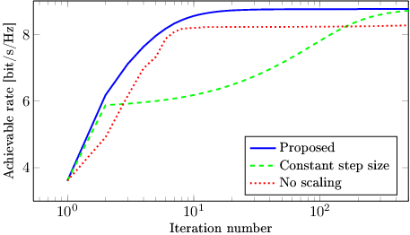
In this subsection, we analyze the influence of data scaling and line search on the PGM. Hence, we compare the proposed PGM with two benchmark schemes. For the first benchmark scheme (i.e., PGM without line search), the PGM is implemented without the line search procedure and we assumed a constant step size equal to 10. For the second benchmark scheme, the PGM is implemented without data scaling. The achievable rate results are shown in Fig. 14. As expected, the proposed PGM has the best achievable rate results among the considered schemes. PGM without line search needs significantly more iterations to reach the optimal achievable rate, for a step size that is multiple times larger than the inverse of the Lipschitz constant (see Theorem 2). Generally, the larger step size enables faster convergence, but the risk of misconvergence is then higher. Furthermore, PGM without data scaling has an achievable rate that is not very significantly worse than the achievable rate of the proposed PGM.
VII Conclusion
In this paper, we proposed a new PGM algorithm for the achievable rate optimization in multi-stream MIMO system equipped with an RIS. Also, we derived a Lipschitz constant that guarantees the convergence of the PGM. To improve the rate of convergence of the PGM algorithm, we proposed a data scaling step and employed a backtracking line search, which enable the PGM to significantly outperform the existing AO algorithm. In addition, we defined the new metric of total FSPL, and showed that the ratio between the total FSPL of the indirect and direct links can successfully serve as a first-order measure of the applicability of an RIS. Numerical results confirm that the PGM requires a significantly lower number of iterations, and correspondingly a substantially lower computational complexity, than the AO in order to reach a target (near-optimal) achievable rate. Furthermore, we showed that the RIS is particularly convenient for application in an indoor environment, since a small number of RIS elements is sufficient to enable the indirect link to have a higher achievable rate than the direct link.
Appendix A Complex-valued Gradient of
We first note that (17b) is given in [30, Eq. (6.207)] and is relatively well known in the related literature. To derive (17a) we follow the procedure to compute the complex-valued gradient of a general function detailed in [30, Sect. 3.3.1]. Note that in the following, we adopt the notations introduced in [30]: denotes the complex differential of . To proceed, we recall that the complex differential of with respect to and is given by
| (41) |
After a few algebraic steps we obtain
| (42) |
where we have used the equality . Let be the matrix used to place the diagonal elements of a square matrix on , i.e. [30, Definition 2.12]. Then we can rewrite as
| (43) |
Using [30, Table 3.2] and [30, Eqn. (2.140)] we obtain
| (44) |
In a similar manner, we can prove the expression for . The details are omitted here due to the page limit.
Appendix B Proof of Lemma 2
To make the proof easy to follow, we first recall the following inequalities, which are well known or can be proved easily. For the norm of a matrix product it holds that
| (45a) | ||||
| (45b) | ||||
where denotes the largest singular value of . Since , we have
| (46) |
It is easy to check that
| (47) |
B-A Proof of (27)
From (17a) we obtain
| (48) |
The first term on the right-hand side of (48) can be upper-bounded as
| (49) |
Furthermore, we have
| (50) |
Substituting (50) into (49) gives
| (51) |
Similarly, the second term on the right-hand side (RHS) of (48) can be upper-bounded as
| (52) |
Furthermore, we obtain
| (53) |
The following inequalities hold for the two norms in the RHS of the above equation:
| (54) |
and
| (55) |
To upper-bound the two terms on the RHS of (55), we use
| (56) |
and
| (57) |
Substituting (54), (55), (56) and (57) into (53), we obtain
| (58) |
and (52) then implies
| (59) |
B-B Proof of (28)
Appendix C Proof of Theorem 2
We recall the following inequality for any function which is -smooth:
| (61) |
The projection of onto can be written as
| (62) |
where and we have used the fact that . Note that when , the objective in the above problem is equal to 0, and thus we have
| (63) |
An analogous inequality also holds for , i.e.,
| (64) |
Applying (61) yields
| (65) |
It is easy to see that if . Since the feasible set of the considered problem is closed and bounded, the iterate is bounded and thus has accumulation points. Since, as shown above, is nondecreasing, has the same value, denoted by , at all of these accumulation points. From (65) we have
| (66) |
which results in
| (67) |
Since we can conclude that
| (68) |
The optimality condition of (62) implies
| (69) |
Similarly we have
| (70) |
Let be any accumulation point of , say as . We also note that the gradient of is continuous and thus and . By letting in (69) and (70), we have
| (71) |
| (72) |
which means that is indeed a critical point of (11). This completes the proof.
Appendix D Computational Complexity for Alternating Optimization (AO)
The computational complexity for the AO method, introduced in [24], is derived in this appendix. To make the following derivation more accessible, the mathematical notation in this appendix is the same as in [24].
The channel matrix from the transmitter to the receiver is given by , where presents the direct signal transmission between the transmitter and the receiver, presents the signal transmission between the transmitter and the RIS, presents the signal transmission between the RIS and the receiver, and models the RIS response. Let , and , so that the channel matrix can be written as .
In the first step of the AO algorithm, independent realizations of are randomly generated and for each of these the optimal covariance matrix is computed. To do this, the channel matrix has to be calculated for every realization. This calculation starts by computing all matrices and for this multiplications are needed. Further, the computation of all matrices requires multiplications (per one realization). Hence, the complexity of calculating channel matrices is .
For each it is required to perform the the truncated singular value decomposition , where and . The complexity of this decomposition is approximately . Next, is computed as , where are obtained using a water-filling algorithm and . The complexity of the water-filling algorithm is and the complexity of the matrix multiplication is . Therefore, the calculation of covariance matrices requires multiplications.
In the sequel, the optimal and are iteratively determined. In one conventional iteration, one or is adjusted. A set of successive conventional iterations constitutes one “outer” iteration, in which all and are adjusted. The AO method stops when the convergence criterion at the end of an outer iteration is fulfilled.
At the beginning of each outer iteration, the eigenvalue decomposition is performed, which requires multiplications. The calculation of the matrices and has the complexity .
To form , multiplications are needed first to obtain all and multiplications are needed for all . Hence, the complexity of computing is .
The optimization of the -th RIS element requires the computation of the following auxiliary matrices
| (73) | ||||
| (74) |
where . It can be easily shown that the complexities for calculating and from the previous expressions are both .
Utilizing the results from Subsection IV-B, the complexity of computing is . The subsequent calculation of and update of require a negligible complexity.
After adjusting all RIS elements, the optimization of is performed according to the aforementioned procedure, which requires multiplications.
If is the number of outer iterations, then the computational complexity of the AO algorithm is given by
| (75) |
where .
References
- [1] M. Di Renzo et al., “Smart radio environments empowered by reconfigurable AI meta-surfaces: An idea whose time has come,” EURASIP J. Wireless Commun. and Netw., vol. 2019, no. 1, pp. 1–20, 2019.
- [2] ——, “Reconfigurable intelligent surfaces vs. relaying: Differences, similarities, and performance comparison,” IEEE Open Jour. of the Commun. Society, vol. 1, pp. 798–807, Jun. 2020.
- [3] E. Basar et al., “Wireless communications through reconfigurable intelligent surfaces,” IEEE Access, vol. 7, pp. 116 753–116 773, 2019.
- [4] C. Huang et al., “Holographic MIMO surfaces for 6G wireless networks: Opportunities, challenges, and trends,” IEEE Wirel. Commun., vol. 27, no. 5, pp. 118–125, Oct. 2020.
- [5] A. Taha et al., “Enabling large intelligent surfaces with compressive sensing and deep learning,” arXiv preprint arXiv:1904.10136, 2019.
- [6] Z.-Q. He and X. Yuan, “Cascaded channel estimation for large intelligent metasurface assisted massive MIMO,” IEEE Wireless Commun. Lett., vol. 9, no. 2, pp. 210–214, Feb. 2020.
- [7] M. Di Renzo et al., “Smart radio environments empowered by reconfigurable intelligent surfaces: How it works, state of research, and road ahead,” IEEE J. Sel. Areas Commun., vol. 38, no. 11, pp. 2450–2525, Nov. 2020.
- [8] F. H. Danufane et al., “On the path-loss of reconfigurable intelligent surfaces: An approach based on Green’s theorem applied to vector fields,” arXiv preprint arXiv:2007.13158, 2020.
- [9] Q. Wu and R. Zhang, “Intelligent reflecting surface enhanced wireless network via joint active and passive beamforming,” IEEE Trans. Wireless Commun., vol. 18, no. 11, pp. 5394–5409, Nov. 2019.
- [10] X. Yu et al., “Robust and secure wireless communications via intelligent reflecting surfaces,” IEEE J. Sel. Areas Commun., vol. 38, no. 11, pp. 2637–2652, Nov. 2020.
- [11] ——, “MISO wireless communication systems via intelligent reflecting surfaces,” in Proc. IEEE/CIC Int. Conf. on Commun. in China (ICCC). IEEE, Aug 2019.
- [12] Q.-U.-A. Nadeem et al., “Asymptotic max-min SINR analysis of reconfigurable intelligent surface assisted MISO systems,” IEEE Trans. Wireless Commun., vol. 19, no. 12, pp. 7748–7764, Dec. 2020.
- [13] P. Wang et al., “Intelligent reflecting surface-assisted millimeter wave communications: Joint active and passive precoding design,” IEEE Trans. Veh. Technol., 2020, Early Access.
- [14] C. Huang et al., “Reconfigurable intelligent surfaces for energy efficiency in wireless communication,” IEEE Trans. Wireless Commun., vol. 18, no. 8, pp. 4157–4170, Aug. 2019.
- [15] ——, “Reconfigurable intelligent surface assisted multiuser MISO systems exploiting deep reinforcement learning,” IEEE J. Sel. Areas Commun., vol. 38, no. 8, pp. 1839–1850, Aug. 2020.
- [16] M.-M. Zhao et al., “Exploiting amplitude control in intelligent reflecting surface aided wireless communication with imperfect CSI,” arXiv preprint arXiv:2005.07002, 2020.
- [17] S. Abeywickrama et al., “Intelligent reflecting surface: Practical phase shift model and beamforming optimization,” IEEE Trans. Commun., vol. 68, no. 9, pp. 5849–5863, Sep. 2020.
- [18] B. Di et al., “Hybrid beamforming for reconfigurable intelligent surface based multi-user communications: Achievable rates with limited discrete phase shifts,” IEEE J. Sel. Areas Commun., vol. 38, no. 8, pp. 1809–1822, Aug. 2020.
- [19] T. Hou et al., “Reconfigurable intelligent surface aided NOMA networks,” IEEE J. Sel. Areas Commun., vol. 38, no. 11, pp. 2575–2588, Nov. 2020.
- [20] Y. Yang et al., “IRS-enhanced OFDMA: Joint resource allocation and passive beamforming optimization,” IEEE Wireless Commun. Lett., vol. 9, no. 6, pp. 760–764, Jun. 2020.
- [21] J. Xiong et al., “Reconfigurable intelligent surfaces assisted MIMO-MAC with partial CSI,” in Proc. IEEE Int. Conf. on Communications (ICC), 2020, pp. 1–6.
- [22] Ö. Özdogan et al., “Using intelligent reflecting surfaces for rank improvement in MIMO communications,” in Proc. IEEE Int. Conf. on Acoustics, Speech and Signal Proc. (ICASSP), 2020, pp. 9160–9164.
- [23] N. S. Perović et al., “Channel capacity optimization using reconfigurable intelligent surfaces in indoor mmWave environments,” in Proc. IEEE Int. Conf. on Communications (ICC), 2020, pp. 1–7.
- [24] S. Zhang and R. Zhang, “Capacity characterization for intelligent reflecting surface aided MIMO communication,” IEEE J. Sel. Areas Commun., vol. 38, no. 8, pp. 1823–1838, Aug. 2020.
- [25] T. S. Rappaport et al., “Overview of millimeter wave communications for fifth-generation (5G) wireless networks–With a focus on propagation models,” IEEE Trans. Antennas Propag., vol. 65, no. 12, pp. 6213–6230, Dec. 2017.
- [26] S. W. Ellingson, “Path loss in reconfigurable intelligent surface-enabled channels,” arXiv preprint arXiv:1912.06759, 2019.
- [27] S. J. Orfanidis, Electromagnetic waves and antennas. Rutgers University New Brunswick, NJ, 2002.
- [28] R. Karasik et al., “Beyond max-SNR: Joint encoding for reconfigurable intelligent surfaces,” in Proc. International Symposium on Information Theory (ISIT), 2020, pp. 2965–2970.
- [29] H. Li and Z. Lin, “Accelerated proximal gradient methods for nonconvex programming,” in Advances in neural information processing systems, 2015, pp. 379–387.
- [30] A. Hjörungnes, Complex-calued matrix derivatives with applications in signal processing and communications. Cambridge University Press, 2011.
- [31] T. M. Pham et al., “Revisiting the MIMO capacity with per-antenna power constraint: Fixed-point iteration and alternating optimization,” IEEE Trans. Wireless Commun., vol. 18, no. 1, pp. 388–401, Jan. 2019.
- [32] S. Lin et al., “Reconfigurable intelligent surfaces with reflection pattern modulation: Beamforming design and performance analysis,” IEEE Trans. Wireless Commun., 2020, Early Access.
- [33] A. Zappone et al., “Overhead-aware design of reconfigurable intelligent surfaces in smart radio environments,” IEEE Trans. Wireless Commun., vol. 20, no. 1, pp. 126–141, Jan. 2021.
- [34] L. Armijo, “Minimization of functions having Lipschitz continuous first partial derivatives,” Pac. J. Math., vol. 16, no. 1, pp. 1–3, 1966.
- [35] X. Qian et al., “Beamforming through reconfigurable intelligent surfaces in single-user MIMO systems: SNR distribution and scaling laws in the presence of channel fading and phase noise,” IEEE Wireless Commun. Lett., vol. 10, no. 1, pp. 77–81, Jan. 2021.