Learning Domain-invariant Graph for Adaptive Semi-supervised Domain Adaptation with Few Labeled Source Samples

Geometric adaptation methods involve a hypothesis that input samples are sampled from a low-dimensional manifold structure, and similar samples should be encoded with similar representations [20, 4]. It aims to better link source and target domains by exploiting the low-dimensional structure which reflects the intrinsic distribution of input samples.

Gong et al. [21] proposed a geometric flow kernel (GFK) method to extract the infinite number of subspaces that change along the geodesic flow across domains. Yao et al. [22] proposed the Semi-supervised Domain Adaptation with Subspace Learning (SDASL) method to find a subspace where the divergence between the source and target mappings of the same class is minimized. And it uses manifold regularization to exploit the intrinsic information of the target domain. Wang et al. [23] proposed the Manifold Embedded Distribution Alignment (MEDA). It introduces manifold feature learning to exploit the geometric property of the data in Grassmann manifold to construct a cross-domain classifier better.

The major restriction of these domain adaptation works is that they seriously rely on a large amount of source label information, which is labor-consuming to collect in real applications. Therefore, we propose DGL to deal with one more practical problem of domain adaptation where only a few labeled source samples are available.

The Nystr$\rm\ddot{o}$m method is initially introduced to seek the solution of integral Eq.1  [19, 24].

where $k(\cdot)$ is a function which is positive semidefinite and square integrable. $p(\cdot)$ is probability density function. $\lambda_{i}$ and $\phi_{i}(\cdot)$ are eigenvalues and eigenfunctions of integral Eq.1.

In the theory of kernel machine analysis, the Nystr$\rm\ddot{o}$m method is employed to approximate the Gram matrix to reduce the computational burden [25, 26, 27]. Given a dataset $\mathrm{T}=\left\{t_{i}\right\}_{i=1}^{n_{1}}$ sampled from the distribution $p(t)$, a kernel matrix $K_{T}$ built based on $\mathrm{T}$. Given another new dataset $\mathrm{S}=\left\{s_{i}\right\}_{i=1}^{n_{2}}$ sampled from the same distribution of $\mathrm{T}$ . The eigenfunction $\phi_{i}(s)$ on new instance $s_{i}$ can be estimated by Eq. 2:

The eigenfunction $\phi_{i}(s)$ on new dataset $\mathrm{S}$ is approximated in a matrix form as follows:

where $\Lambda_{T}=\operatorname{diag}\left(\lambda_{1},\ldots,\lambda_{n_{1}}\right)\in R^{n_{1}\times n_{1}}$ are $n_{1}$ eigenvalues and $\Phi_{T}\in R^{n_{1}\times n_{1}}$ are $n_{1}$ eigenvectors of $K_{T}$, i.e., $K_{T}=\Phi_{T}\Lambda_{T}\Phi_{T}^{T}$. $K_{S,T}\in R^{n_{2}\times n_{1}}$ is the similarity matrix between two datasets. $\Phi_{S}\in R^{n_{2}\times n_{1}}$ is the extrapolated eigenvector matrix of kernel matrix $K_{S}$ . The kernel matrix $K_{S}$ can be estimated by Eq.4:

Attracted by the properties and successful applications of the Nystr$\rm\ddot{o}$m method, we flexibly apply it to domain adaptation and use it to discuss geometric relationships between domains. By flexibly employing the Nystr$\rm\ddot{o}$m method, we build a domain-invariant graph to bridge two domains geometrically. To our best knowledge, it is the first attempt for transfer learning with such a strategy.

Suppose there are $n_{t}$ samples $X_{t}=\left\{x_{i}^{t}\right\}_{i=1}^{n_{t}}\in R^{m\times n_{t}}$ in target domain $D_{t}$, and $n_{s}$ samples $X_{s}=\left\{x_{i}^{s}\right\}_{i=1}^{n_{s}}\in R^{m\times n_{s}}$ in source domain $D_{s}$. Specifically, source domain includes $u$ unlabeled samples $X_{t}^{u}=\left\{x_{i}^{su}\right\}_{i=1}^{u}\in R^{m\times u}$ and $l$ labeled samples $X_{s}^{l}=\left\{x_{i}^{sl}\right\}_{i=1}^{l}\in R^{m\times l}$ $(u\gg l,u+l=n_{s})$. Denote $Y_{s}$ as the source label matrix. In DGL, only scarce source label information can be available, referring to $Y_{s}^{l}{=\left\{y_{i}^{sl}\right\}}_{i=1}^{l}$. Generally, the data of two domains are generated from the identical $m$ dimension feature space with the same $C$ classes. But they have different marginal probability distribution, i.e., $\mathcal{P}_{s}\neq\mathcal{P}_{t}$.

Let ${{L}^{\centerdot}}$ represents a source or target graph Laplacian ( $\centerdot$ can be either source or target) and ${{\Phi}^{\centerdot}}$ and ${{\Lambda}^{\centerdot}}$ represent the eigenvector and eigenvalue matrices of graph Laplacian ${{L}^{\centerdot}}$ respectively. In the following sections, we compute the Laplacian matrix as $L^{\centerdot}=D^{\centerdot}-W^{\centerdot}$, where $W^{\centerdot}$ is the affinity matrix given by Gaussian kernel $k$ with the form $W_{ij}^{\centerdot}=\exp\left({-\left\|x_{i}^{\centerdot}-x_{j}^{\centerdot}\right\|_{2}^{2}}/{2{{\sigma}^{2}}}\;\right)$. $\sigma$ is bandwidth and fixed 1 in this paper. $D^{\centerdot}$ is the diagonal matrix computed by $D_{ij}^{\centerdot}=\sum_{j=1}^{\ }W_{ij}^{\centerdot}$.

DGL is proposed to address a new problem of domain adaptation where only a few labeled source samples are available. Specifically, DGL geometrically links the source and target domains via a domain-invariant graph Laplacian ${{\bar{L}}^{s*}}$. More specifically, DGL uses the Nystr$\rm\ddot{o}$m method to build a plastic graph ${\bar{L}}^{s}$, which has the similar geometric property of target graph. Then DGL utilizes the Nystr$\rm\ddot{o}$m approximation error to measure the divergence between the plastic graph ${\bar{L}}^{s}$ and source graph $L^{s}$ to formalize the distribution mismatch. Finally, the domain-invariant graph can be successfully learnt via minimizing Nystr$\rm\ddot{o}$m method approximation error and naturally integrated into the semi-supervised framework based on source data with the promising performance for target data.

Using the squared loss $V\left(f\left(x_{i}^{sl}\right),y_{i}^{sl}\right)=\left(y_{i}^{sl}-f\left(x_{i}^{sl}\right)\right)^{2}$ and the “Representer Theorem”, the objective 11 based on RLS can be formulated as follows:

where $\boldsymbol{\alpha}=\left(\alpha_{1},...,\alpha_{n_{s}}\right)^{T}$ is the coefficient matrix. $J$ is a diagonal matrix given by $J=diag\left(1,...,1,0,...,0\right)\in R^{n_{s}\times n_{s}}$ with the first $l$ diagonal elements as 1 and the rest 0. $Y_{s}$ is the label matrix on source data. It does not matter that some source label information is unknown, because they can be filtered out by the label indicator matrix $J$. $K\in R^{\left(l+u\right)\times\left(l+u\right)}$ is the Gram matrix over all source data. To simplify calculations, we choose Gaussian kernel function $k$ to compute the Gram matrix in this paper.

The derivative of the objective function is set to 0 and we can obtain:

Denote $y\in R^{C}$ as label vector, then $y_{c}=1$ if $y\left(x\right)=c$ and otherwise $y_{c}=0$. The label matrix $Y_{s}=\left[y_{1}^{s},...,y_{n_{s}}^{s}\right]\in R^{C\times n_{s}}$, and the parameter matrix $\boldsymbol{\alpha}\in R^{n_{s}\times C}$. In such a way, the adaptive classifier based on DGL can be used to deal with the multi-class problem.

Using the hinge loss: $V\left(f\left(x_{i}^{sl}\right),y_{i}^{sl}\right)=\max\left(0,1-y_{i}^{sl}f\left(x_{i}^{sl}\right)\right)$ and the “Representer Theorem”, the objective 11 based on SVM can be formulated as follows:

where $b$ is the bias term, $\xi_{i}$ is the slack variable.

Equation 15 can be effectively solved using the Lagrange dual [20]. Therefore, we can obtain:

where $\boldsymbol{\beta}$ is Lagrange multipliers matrix, $Q=\hat{Y}\hat{J}K\left(2\lambda_{1}I+2\lambda_{2}{\bar{L}}^{s\ast}K\right)^{-1}{\hat{J}}^{T}\hat{Y}$, $\hat{Y}=diag\left(y_{1}^{sl},...,y_{l}^{sl}\right)$, $\hat{J}=\left[I_{l},\mathbf{0}\right]\in R^{l\times\left(l+u\right)}$ , and $I_{l}\in R^{l\times l}$ is the identity matrix.

The adaptive SVM classifier can be easily constructed by using a standard SVM solver with the quadratic form induced by $Q$. Then the obtained $\boldsymbol{\beta}$ is used to solve the parameter $\boldsymbol{\alpha}$ by $\boldsymbol{\alpha}=\left(2\lambda_{1}I+2\lambda_{2}\bar{L}^{s*}K\right)^{-1}\tilde{J}^{T}\hat{Y}\boldsymbol{\beta}$.

The complete procedure of DGL with hinge or squared loss is summarized in Algorithm 1.

The computational complexity of the model includes three parts.

For build ${\bar{L}}^{s\ast}$, computing graph Laplacian costs $\mathcal{O}\left(m\left(n_{s}+n_{t}\right)^{2}\right)$, achieving the eigensystem of $L^{t}$ costs $\mathcal{O}\left(\left(n_{t}\right)^{3}\right)$, estimating eigenvectors of ${\bar{L}}^{s\ast}$ costs $\mathcal{O}\left(n_{s}\left(n_{t}\right)^{2}\right)$, and solving optimal problem for $\Lambda^{\ast}$ costs $\mathcal{O}\left(2\left(n_{t}\right)^{3}\right)$.

Solving the objective 14 using LU decomposition costs $O\left(\left(n_{s}\right)^{3}\right)$. Solving the SVM optimization 16 with the SVM solver [29] costs $\mathcal{O}\left(\left(n_{s}\right)^{2.3}\right)$. For constructing the kernel matrix $K$ costs $\mathcal{O}\left(m\left(n_{s}+n_{t}\right)^{2}\right)$.

Therefore, in summary, the computational complexity of Algorithm 1 is $\mathcal{O}\left(m\left(n_{s}+n_{t}\right)^{2}+\left(n_{t}\right)^{3}+n_{s}\left(n_{t}\right)^{2}+\left(n_{s}\right)^{3}\right)$.

We roughly explained the differences between the proposed DGL and other existing methods in Section II. DGL is substantially different from the prior proposed domain adaptation methods, such as [21, 16, 23]. All these methods rely on large amounts of source label information, which limits their application in real situations. In this subsection, we specifically discuss the differences between DGL and other methods from an insightful perspective.

1. 1.

   Distribution mismatch reduction: The distribution divergence between domains is the fundamental challenge to generalize the source model to the target domain. Therefore, formalizing the distribution mismatch and designing useful strategies to minimize it is the most crucial thing in domain adaptation. Maximum Mean Discrepancy (MMD)[30], as a nonparametric measurement, has been widely used in many domain adaptation methods to compare the distribution distance[31, 23]. However, MMD highly depends on the nonlinear kernel map, and the kernel function may be not optimal for different transfer situations.

2. 2.

   Scope of application: Almost all the prior methods are feasible with a precondition, i.e., enough source label information is available. Although we have rich data resources in practical applications, the label information is seriously insufficient. From this perspective, it is difficult to promote the methods that rely on large amounts of labeled data in practical applications.

DGL is completely different from the prior methods.

1. 1.

   DGL flexibly uses the Nystr$\rm\ddot{o}$m approximation error to formalize the distribution mismatch in a convenient way. DGL has the different perspectives to analyze the connection between domains and finally uses the learnt domain-invariant graph to link two domains geometrically.

2. 2.

   Different from prior methods, the implementation process of DGL does not need to rely on a large amount of label information of source data, thereby broadening the scope of application of DGL. Even when the label information is sufficient, DGL can still achieve comparable accuracy.

In summary, DGL can simultaneously explore the distribution divergence minimization and the challenge of domain adaption, where only a few labeled source data are available. Moreover, DGL is a general idea in which the standard methods can be easily integrated.

Reuters-21578 is a challenging text dataset with many categories. There are three top categories including orgs, people, and place. We directly adopt the preprocessed Reuters-21578 dataset by Gao et al. [32], and build three transfer tasks including “org vs people”, “people vs place” and “org vs place”.

Office and Caltech-256 are are two standard image datasets widely used to evaluate the domain adaptation methods. Office [33, 34] comprises of three object domains, Amazon (A), Webcam (W), and DSLR (D). Amazon contains image downloaded from online merchants, Webcam includes low-resolution images, and DSLR consists of high-resolution images. There are totally 4652 images and 31 categories. Caltech-256 [35] includes 30607 images and 256 categories. We use the public Office+Caltech dataset with SURF features released by Gong et al. [21] in these experiments. Finally, we build twelve transfer tasks, e.g., “A vs C”, “A vs D”, “A vs W”.

To evaluate the performance of DGL, we choose several competitive domain adaptation algorithms to compare with DGL on different transfer tasks.

• •

  Regularized Least Squares (RLS)

• •

  Support Vector Machine (SVM)

• •

  Transfer Component Analysis (TCA)  [3]

• •

  Geodesic Flow Kernel (GFK)  [21]

• •

  Transfer Kernel Learning (TKL)  [16]

• •

  Transfer Joint Matching (TJM)  [36]

• •

  Joint Geometrical and Statistical Alignment (JGSA)  [37]

• •

  Balanced Distribution Adaptation (BDA)  [38]

• •

  Guide Subspace Learning (GSL)  [39]

RLS and SVM are two standard learning algorithms, which can be treated as the special cases of DGL_RLS and DGL_SVM, i.e., $\lambda_{2}=0$. TCA, GFK, TKL, TJM, JGSA, BDA, and GSL are competitive domain adaptation frameworks. Specifically, TCA aims to find a shared subspace by minimizing maximum mean discrepancy across domains. TJM aims to construct new data representations by matching the features and reweighting data across domains. JGSA learns two projections that project the domain data into the subspaces where the geometrical and distribution shifts are reduced. BDA aims to build a shared subspace via minimizing the marginal and conditional distribution discrepancies adaptively. GSL proposes to learn an invariant and discriminative domain agnostic subspace where the distribution mismatch can be minimized.

We randomly sample 5%, 10%, 25%, 50% of source samples as labeled source samples, and the remaining samples are unlabeled. No label information is available in the target domain. For all the methods, we will conduct these methods based on different percents of labeled source samples and test them in the target domain. All experiments are repeated five runs, and we finally take the average of the experimental results.

The parameters of all comparison methods are set as suggested in their original papers. In DGL, there are three main parameters, i.e., $\lambda_{1}$, $\lambda_{2}$ and $\xi$. We tune these parameters in the case of 5$\%$ labeled source samples. Specifically, $\lambda_{1}$ and $\lambda_{2}$ are tuned in a range $\left\{0.001,0.005,0.01,0.05,0.1,0.5,1,5,10\right\}$. $\xi$ is tuned in a range $\left\{1,\ 1.1,1.2,1.3,1.5,2,2.5,3,5\right\}$. The best results are reported, for image datasets $\lambda_{1}=10$, $\lambda_{2}=0.001$, $\xi=1$ and for text datasets $\lambda_{1}=5$, $\lambda_{2}=0.001$,$\ \xi=2$.

We utilize classification accuracy on target data as the evaluation metric [40, 41].

where $f\left(x_{i}\right)$ is the prediction label of target sample $x_{i}$, $y\left(x_{i}\right)$ is the ground truth label of $x_{i}$.

We illustrate the experimental results and provide a brief analysis of them.

The experiment results are shown in Table I-Table IV. Each Table shows the average accuracy of the experiment results in different transfer tasks with different label rates. The best experimental results are shown in bold. Moreover, in order to further observe the effectiveness of DGL. We build another seven transfer tasks where only 5% source label information can be available. From these results, we can make the following analysis.

Firstly, from Table I, we observe that TCA, TKL, GFK, TJM, JGSA, BDA, and GSL these domain methods fail to predict target data in all of the transfer tasks when 5% labeled source data are available during transfer process. A major limitation of these methods is that they rely on large amounts of source label information. In real applications, it is time-consuming and labor-costing to collect large amounts of labeled source samples and thus results in their poor performance when there is scarce label information existing in the source domain. However, DGL can ensure classification accuracy with a few labeled source samples. That is because the domain-invariant graph enables the classifier constructed on source domain to be adaptive to target domain. At the same time, this invariant graph enables DGL to employ unlabeled source samples to assist knowledge transfer, thereby reducing reliance on source label information.

Secondly, from the Table I, DGL achieves much better performance than the baseline methods. we can find that the average classification accuracy of DGL on the different transfer tasks is 46.45%. The accuracy improves 3.84% compared to the best baseline method GFK. Similarly, from the Table 2 to Table 3, the average classification accuracy of DGL with different source label rate is 48.75% and 50.69% respectively. The accuracy improves 1.24% and 1.12% compared to the best baseline method TKL. From the Table 4, with the increase of labeled source data, DGL can still achieve comparable performance than GSL.

Thirdly, the standard RLS and SVM classifiers perform poorly on many transfer tasks. Both methods treat the data from different domains as if they are drawn from the identical distribution. However, this strict assumption is invalid in the real world and therefore results in their poor performance in cross-domain classification problems.

Further analysis of DGL can be observed in Fig. 1. We build another six transfer tasks where only 5% source label information can be available to analyze the effectiveness of DGL further. From Fig. 1, we can find that DGL outperforms the baseline methods in most cases. Moreover, we can observe that in some transfer tasks, the traditional learning method RLS or SVM performs better than some comparison domain adaptation methods. For example, in transfer tasks ¡°C vs D¡±, RLS performs better than TJM, JGSA, BDA, and GSL. We analyze that when there is not enough source label information, implementing knowledge transfer across domains compulsorily will lead to a severe decline in algorithm performance, also known as the negative transfer. However, DGL can achieve stable performance even though there is scarce source label information. Since the analysis is concluded from a large number of experiments, it convincingly demonstrates that DGL can build a robust adaptive classifier for the target domain, especially when there is scarce source label information.

In order to further analyze the influence of source label information in different transfer learning methods, we illustrate the accuracy of different methods with different source label information, referring to Fig. 2. From Fig. 2, we find that the performance of all domain adaptation methods is growing better with increasing source label information. However, we observe that the performance “TKL” and “GSL” increases steeper than the other methods. This shows that these algorithms are more dependent on the source domain label information. We can also find that DGL increases stably with the growing label information, which shows that DGL has strong adaptability and stability. That means DGL can implement knowledge transfer without relying on much source label information and can also achieve comparable performance than the baseline method with increasing label information.

However, from the trend in the Fig. 2, we speculate that when the source domain label rate reaches 100%, the performance of DGL is not necessarily significantly better than other methods. We think that when source domain label information is sufficient, merely considering the geometric connection between domains is not enough. Maybe some statistical information, e.g., means, the variance should also be adapted between domains. We will analyze it in our future work, because the fundamental point of DGL is to solve the problem of domain adaptation with only scarce source label information. From all experimental results, we can observe that DGL can successfully implement knowledge transfer across domains with scarce source label information.

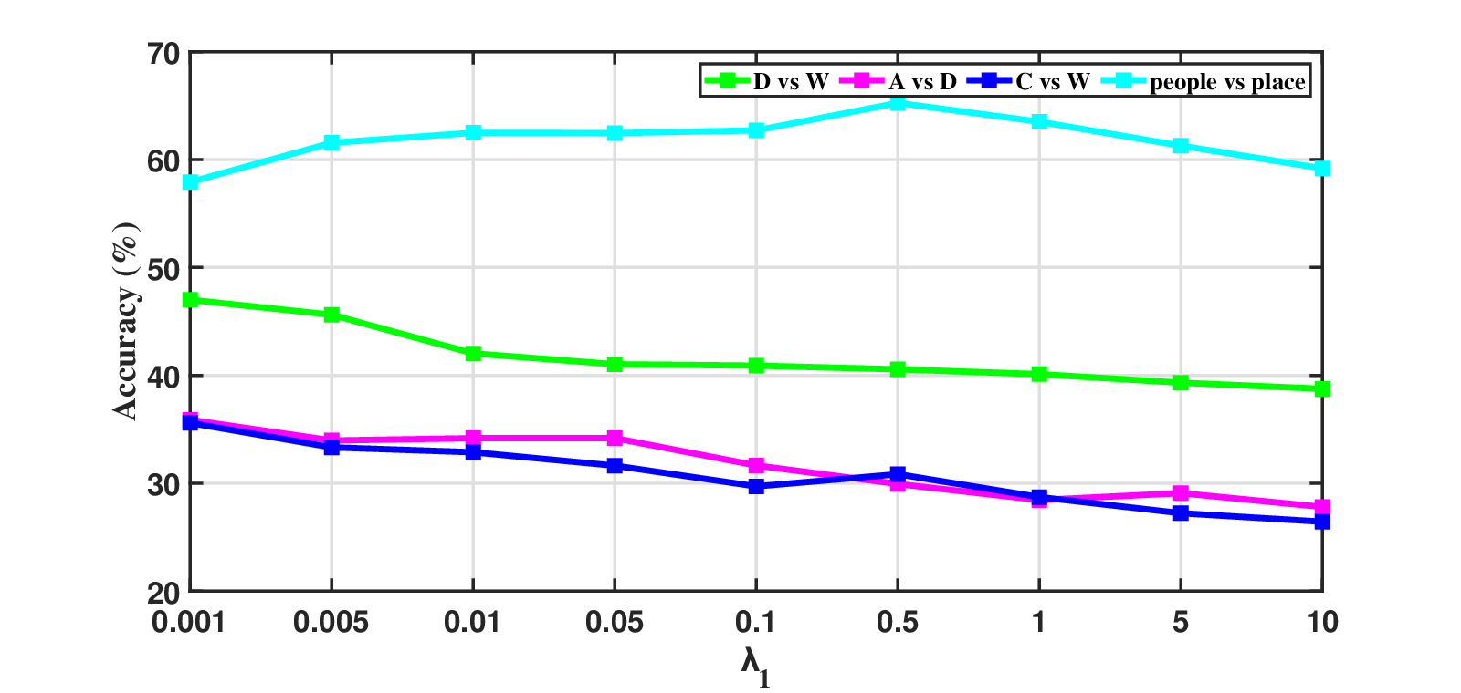
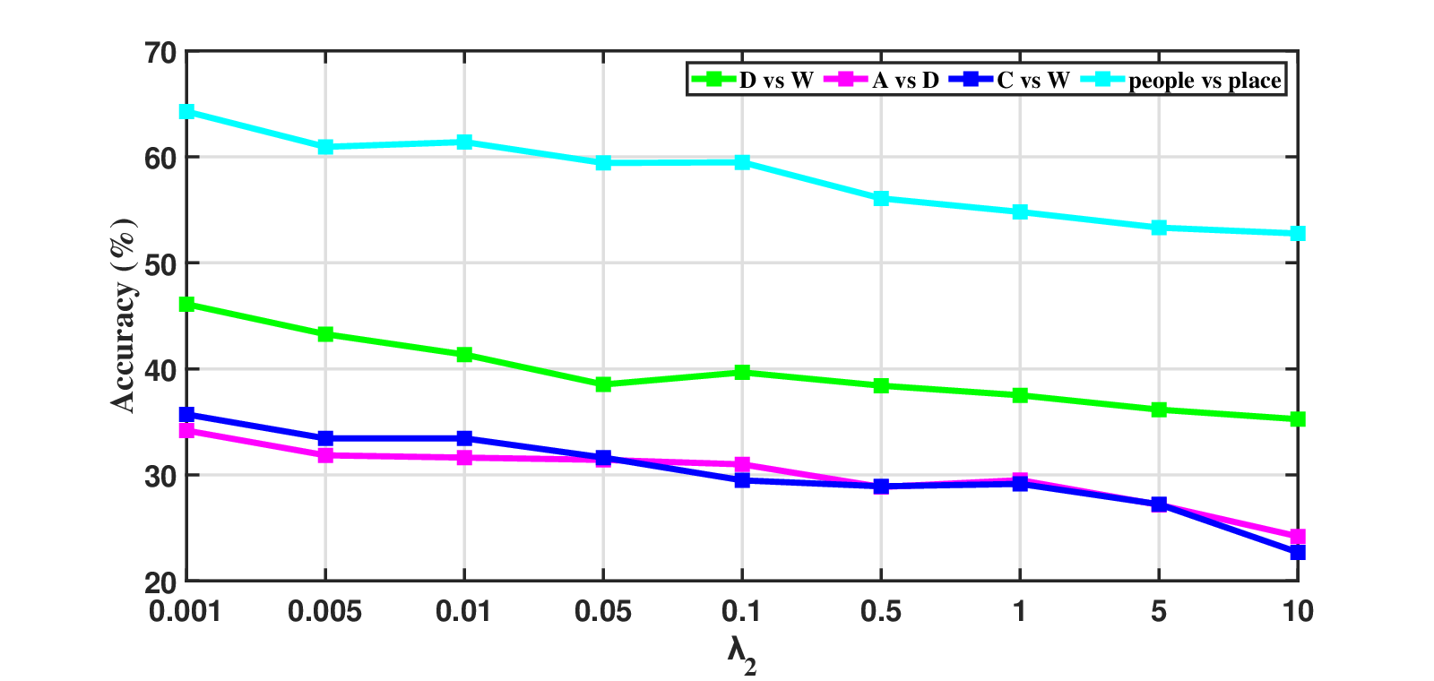
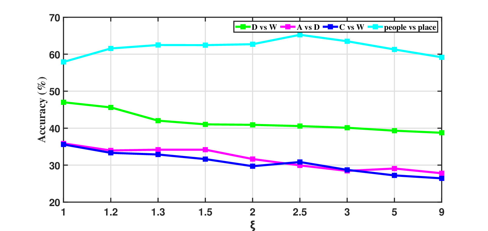
In DGL approach, three parameters should be tuned: classifier complexity controlling parameter $\lambda_{1}$, geometric adaptation parameter$\lambda_{2}$ and damping parameter $\xi$. We randomly conduct parameter sensitivity on “D vs W”, “A vs D”, “C vs W”, and “people vs place” transfer tasks. 5% source samples are selected as labeled samples. We implement DGL with the varying values of $\lambda_{1}\in\left[0.001,10\right]$ by fixing $\lambda_{2}$ and $\xi$. Similar settings are conducted with $\lambda_{2}\in\left[0.001,10\right]$ and $\xi\in\left[1,5\right]$. All results are illustrated in Fig. 3 (a)-(c). $\lambda_{1}$ is used to control the classifier complexity. From the plots, we observe that DGL can perform stably under a wide range $\lambda_{1}\in\left[1,10\right]$. $\lambda_{2}$ is used to control the geometric adaptation. We plot classification accuracy with different values of $\lambda_{2}$. We find that DGL is a little sensitive to the $\lambda_{2}$, and the best results can be obtained when $\lambda_{2}=0.001$. $\xi$ can be used to control the decaying trend of the eigen-spectrum. For text dataset, we can choose $\xi\in\left[1.5,2.5\right]$ for stable performance. For image dataset, DGL is a little sensitive to $\xi$, and the best results can be achieved when $\xi=1$.

References

- [1] S. J. Pan and Q. Yang, “A survey on transfer learning,” IEEE Transactions on Knowledge and Data Engineering, vol. 22, no. 10, pp. 1345–1359, 2010.
- [2] L. Zhang, “Transfer adaptation learning: A decade survey,” CoRR, vol. abs/1903.04687, 2019. [Online]. Available: http://arxiv.org/abs/1903.04687
- [3] S. J. Pan, I. W. Tsang, J. T. Kwok, and Q. Yang, “Domain adaptation via transfer component analysis,” IEEE Transactions on Neural Networks, vol. 22, no. 2, pp. 199–210, 2011.
- [4] M. Long, J. Wang, G. Ding, D. Shen, and Q. Yang, “Transfer learning with graph co-regularization,” IEEE Transactions on Knowledge and Data Engineering, vol. 26, no. 7, pp. 1805–1818, 2014.
- [5] K. Yan, L. Kou, , and D. Zhang, “Learning domain-invariant subspace using domain features and independence maximization,” IEEE Transactions on Cybernetics, vol. 48, no. 1, pp. 288–299, 2018.
- [6] P. Wei, Y. Ke, , and C. Goh, “A general domain specific feature transfer framework for hybrid domain adaptation,” IEEE Transactions on Knowledge and Data Engineering, vol. 31, no. 8, pp. 1440–1451, 2019.
- [7] H. Wang, F. Nie, H. Huang, and C. Ding, “Dyadic transfer learning for cross-domain image classification,” in Proceedings of the IEEE International Conference on Computer Vision (ICCV), 2011, pp. 551–556.
- [8] L. Zhang, J. Yang, and D. Zhang, “Domain class consistency based transfer learning for image classification across domains,” Information Sciences, vol. 418-419, pp. 242–257, 2017.
- [9] Z. Ding and Y. Fu, “Robust transfer metric learning for image classification,” IEEE Transactions on Image Processing, vol. 26, no. 2, pp. 660–670, 2017.
- [10] F. Zhuang, P. Luo, Z. Shen, Q. He, Y. Xiong, Z. Shi, , and H. Xiong, “Mining distinction and commonality across multiple domains using generative model for text classification,” IEEE Transactions on Knowledge and Data Engineering, vol. 24, no. 11, pp. 2025–2039, 2012.
- [11] R. Zhao and K. Mao, “Supervised adaptive-transfer plsa for cross-domain text classification,” in Proceedings of the IEEE International Conference on Data Mining Workshops (ICDMW), 2014, pp. 259–266.
- [12] Y. Li, B. Wei, L. Yao, H. Chen, and Z. Li, “Knowledge-based document embedding for cross-domain text classification,” in Proceedings of the International Joint Conference on Neural Networks (IJCNN), 2017, pp. 1395–1402.
- [13] W. Dai, Q. Yang, G. Xue, and Y. Yu, “Boosting for transfer learning,” in Proceedings of the International Conference on Machine learning (ICML), 2007, pp. 193–200.
- [14] W. Chu, F. Torre, and J. F. Cohn, “Selective transfer machine for personalized facial expression analysis,” IEEE Trans. Pattern Anal. Mach. Intell., vol. 39, no. 3, pp. 529–545, 2017.
- [15] S. Chen, F. Zhou, and Q. Liao, “Visual domain adaptation using weighted subspace alignment,” in Proceedings of the Visual Communications and Image Processing, (VCIP), 2016.
- [16] M. Long, J. Wang, J. Sun, and P. S. Yu, “Domain invariant transfer kernel learning,” IEEE Transactions on Knowledge and Data Engineering, vol. 27, no. 6, pp. 1519–1532, 2015.
- [17] D. Das and C. S. G. Lee, “Graph matching and pseudo-label guided deep unsupervised domain adaptation,” in In Proceedings of the International Conference on Artificial Neural Networks (ICANN), 2018, pp. 342–352.
- [18] N. Courty, R. Flamary, D. Tuia, and A. Rakotomamonjy, “Optimal transport for domain adaptation,” IEEE Transactions on Pattern Analysis and Machine Intelligence, vol. 39, no. 9, 2015.
- [19] K. Zhang, I. W. Tsang, and J. T. Kwok, “Improved nystrm low-rank approximation and error analysis,” in Proceedings of the International Conference on Machine learning (ICML), 2008, pp. 1232–1239.
- [20] M.Belkin, P. Niyogi, and V. Sindhwani, “Manifold regularization: A geometric framework for learning from labeled and unlabeled examples,” Journal of Machine Learning Research, vol. 7, pp. 2399–2434, 2006.
- [21] B. Gong, Y. Shi, F. Sha, and K. Grauman, “Geodesic flow kernel for unsupervised domain adaptation,” in Proceedings of the IEEE Conference on Computer Vision and Pattern Recognition (CVPR), 2012, pp. 2066–2073.
- [22] T. Yao, Y. Pan, C. Ngo, H. Li, and T. Mei, “Semi-supervised domain adaptation with subspace learning for visual recognition,” in Proceedings of the IEEE Conference on Computer Vision and Pattern Recognition (CVPR), 2015, pp. 2142–2150.
- [23] J. Wang, W. Feng, Y. Chen, H. Yu, M. Huang, and P. S. Yu, “Visual domain adaptation with manifold embedded distribution alignment,” in In Proceedings of the ACM International Conference on Multimedia (ACMMM), 2018.
- [24] C. Fowlkes, S. Belongie, F. Chung, and J. Malik, “Spectral grouping using the nystrom method,” IEEE Transactions on Pattern Analysis and Machine Intelligence, vol. 26, no. 2, pp. 214–225, 2004.
- [25] C. Williams and M. Seeger, “Using the nystrm method to speed up kernel machines,” in In Proceedings of Advances in Neural Information Processing Systems (NIPS), 2000, pp. 682–688.
- [26] P. Drineas and M. Mahoney, “On the nystrm method for approximating a gram matrix for improved kernel-based learning,” Journal of Machine Learning Research, vol. 6, pp. 2153–2175, 2005.
- [27] M. Li, W. Bi, J. Kwok, and B. Lu, “Large-scale nystrm kernel matrix approximation using randomized svd,” IEEE Transactions on Neural Networks and Learning System, vol. 26, no. 1, pp. 152–164, 2015.
- [28] M. Andersen, J. Dahl, Z. Liu, and L. Vandenberghe, Interior-point methods for large-scale cone programming, 2011.
- [29] C. Chih-Chung and L. Chih-Jen, “Libsvm: a library for support vector machines,” ACM Trans. Intell. Syst. Technol., vol. 2(3), pp. 1–27, 01 2011.
- [30] A. Gretton, K. M. Borgwardt, M. J. Rasch, B. Schölkopf, and A. J. Smola, “A kernel method for the two-sample-problem,” in Proceedings of the Advances in Neural Information Processing Systems, 2006, pp. 513–520.
- [31] M. Long, J. Wang, G. Ding, S. J. Pan, and P. S. Yu, “Adaptation regularization: A general framework for transfer learning,” IEEE Transactions on Knowledge and Data Engineering, vol. 26, no. 5, pp. 1076–1089, 2014.
- [32] J. Gao, W. Fan, J. Jiang, and J. Han, “Knowledge transfer via multiple model local structure mapping,” in The ACM SIGKDD international conference on Knowledge discovery and data mining (KDD), 2008, pp. 283–291.
- [33] W.Li, L. Duan, D. Xu, , and I. W. Tsang, “Learning with augmented features for supervised and semi-supervised heterogeneous domain adaptation,” IEEE Transactions on Pattern Analysis and Machine Intelligence, vol. 36, no. 6, pp. 1134–1148, 2014.
- [34] H. Liu, M. Shao, Z. Ding, and Y. Fu, “Structure-preserved unsupervised domain adaptation,” IEEE Transactions on Knowledge and Data Engineering, vol. 31, no. 4, pp. 799–812, 2019.
- [35] G. Griffin, A. Holub, and P. Perona., “Caltech-256 object category dataset,” CalTech Report, 2007.
- [36] M. Long, J. Wang, G. Ding, J. Sun, and P. S. Yu, “Transfer joint matching for unsupervised domain adaptation,” in Proceedings of the IEEE Conference on Computer Vision and Pattern Recognition (CVPR), 2014, pp. 1410–1417.
- [37] J. Zhang, W. Li, and P. Ogunbona, “Joint geometrical and statistical alignment for visual domain adaptation,” in Proceedings of the IEEE Conference on Computer Vision and Pattern Recognition (CVPR), 2017, pp. 5150–5158.
- [38] J. Wang, Y. Chen, S. Hao, W. Feng, and Z. Shen, “Balanced distribution adaptation for transfer learning,” in Proceedings of the IEEE International Conference on Data Mining (ICDM), 2017, pp. 1129–1134.
- [39] L. Zhang, J. Fu, S. Wang, D. Zhang, Z. Y. Dong, and C. L. P. Chen, “Guide subspace learning for unsupervised domain adaptation,” IEEE Transactions on Neural Networks and Learning Systems, pp. 1–15, 2019.
- [40] L. Duan, I. Tsang, and D. Xu, “Domain transfer multiple kernel learning,” IEEE Transactions on Pattern Analysis and Machine Intelligence, vol. 34, no. 3, pp. 465–479, 2012.
- [41] W. Jiang, H. Gao, W. Lu, W. Liu, F. Chung, and H. Huang, “Stacked robust adaptively regularized auto-regressions for domain adaptation,” IEEE Transactions on Knowledge and Data Engineering, vol. 31, no. 3, pp. 561–574, 2019.