Explainable Recommender Systems via Resolving
Learning RepresentationsConference: Proceedings of the 29th ACM International Conference on Information and Knowledge Management; October 19–23, 2020; Virtual Event, IrelandProceedings of the 29th ACM International Conference on Information and Knowledge Management (CIKM ’20), October 19–23, 2020, Virtual Event, IrelandPrice: 15.00DOI: 10.1145/3340531.3411919ISBN: 978-1-4503-6859-9/20/10
Abstract.
Recommender systems play a fundamental role in web applications in filtering massive information and matching user interests. While many efforts have been devoted to developing more effective models in various scenarios, the exploration on the explainability of recommender systems is running behind. Explanations could help improve user experience and discover system defects. In this paper, after formally introducing the elements that are related to model explainability, we propose a novel explainable recommendation model through improving the transparency of the representation learning process. Specifically, to overcome the representation entangling problem in traditional models, we revise traditional graph convolution to discriminate information from different layers. Also, each representation vector is factorized into several segments, where each segment relates to one semantic aspect in data. Different from previous work, in our model, factor discovery and representation learning are simultaneously conducted, and we are able to handle extra attribute information and knowledge. In this way, the proposed model can learn interpretable and meaningful representations for users and items. Unlike traditional methods that need to make a trade-off between explainability and effectiveness, the performance of our proposed explainable model is not negatively affected after considering explainability. Finally, comprehensive experiments are conducted to validate the performance of our model as well as explanation faithfulness.
Keywords:
Explainable Artificial Intelligence; Recommender Systems1. Introduction
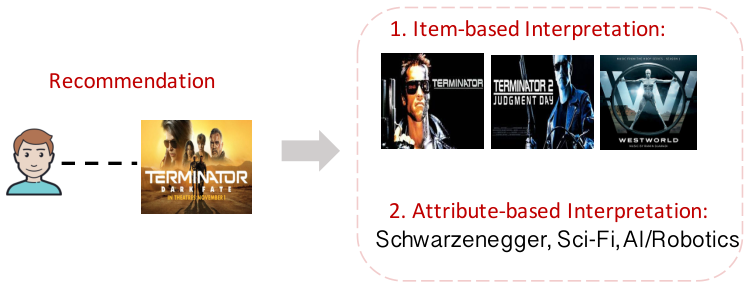
Recommender systems play a pivotal role in a wide range of web applications and services, in terms of distributing online content to targets who are likely to be interested in it. The majority of the efforts in the domain have been put into developing more effective models to achieve better performance. In contrast, the progress of analyzing the explainability aspect of recommender systems is running behind. Explainable recommender systems address the problem of why – besides providing recommendation results, they also give reasons to clarify why such results are derived (Zhang and Chen 2018; Yang et al. 2018a; Gunning and Aha 2019; Ribeiro et al. 2016). Explainability may benefit a recommender system in several aspects. First, explanations help system maintainers to diagnose and refine the recommendation pipeline (system-oriented). Second, by increasing transparency, explanations promote persuasiveness and customer satisfaction of recommender systems (user-oriented).
Recently, Explainable AI (XAI), or interpretable machine learning, is receiving increasing attention (Gunning and Aha 2019; Du et al. 2018; Montavon et al. 2018) (we use "explanation" and "interpretation" interchangeably in this paper). One popular direction is post-hoc methods (Du et al. 2018; Ribeiro et al. 2016), where some examples include understanding the meaning of latent factors (Peake and Wang 2018; Guan et al. 2019) or reconstructing the rationale behind each prediction (Yang et al. 2018a). However, post-hoc interpretation suffers from the issue of explanation accuracy (Rudin 2019; Gunning and Aha 2019). Another direction is to build explainable models or add explainable components, where attention mechanism is commonly applied to highlight important features for prediction (Seo et al. 2017; Gao et al. 2019). Nevertheless, explanation schemes such as heatmaps in images or texts are not structured and still require subjective comprehension of users. Since effective models can learn informative latent representations from data (Bengio et al. 2013; Higgins et al. 2017; Sabour et al. 2017), one of the important building blocks of model explainability is the transparency of representation learning. In traditional factorization models, input features can be directly associated with latent factors to elucidate their meanings (Zhang et al. 2014), but this explanation scheme is not directly applicable to recent embedding learning frameworks.
In this work, we propose an explainable recommendation model through promoting the transparency of latent representations. To begin with, we summarize three elements that help make a model more interpretable. We name them as IOM elements since they involve certain requirements on the Input data format, Output attribution, and Middle-level representations. The proposed explainable model is designed based on the IOM elements. Users, items and attribute entities are processed as nodes in a graph. Furthermore, the efforts on interpretable recommendation are split into three parts: (1) we disentangle the interactions between latent representations in different layers; (2) multiple semantic factors are identified automatically from data; (3) latent dimensions are divided into segments according to their information source (i.e., node types) and affiliated factors. The first part is achieved via graph convolutional networks (GCNs). However, different from previous work (Hamilton et al. 2017b; Wang et al. 2019a; Wang et al. 2019e), we propose to understand GCNs from another perspective by comparing its working mechanism with those of fully-connected networks (Cheng et al. 2016) and capsule networks (Sabour et al. 2017). The second and third aspects are achieved through a novel architecture design, where different dimensions of latent representations focus on different aspects of data. Different from previous work (Epasto and Perozzi 2019; Liu et al. 2019; Wang et al. 2019c), factor discovery and representation learning are jointly conducted. In this way, we are able to depict how information flows from input features through these latent states to prediction results. Different from some existing work that sacrifices effectiveness for interpretability, the proposed model still achieves good performance in the experimental evaluation. Finally, besides visualizing explanations, we also quantitatively measure explanation accuracy.
Our contributions in this work are summarized as follows:
- •
We propose an explainable recommendation model that improves transparency of latent representations. Specifically, we propose to unravel the interactions between representations, and segment the latent dimensions into different factors. The consideration of interpretability does not negatively influence model effectiveness.
- •
We summarize and refine the elements that improve the interpretability of recommendation. These elements involve certain requirements on the input data format, output attribution, and middle-level representations, and are thus named as IOM elements. The proposed model is designed based on IOM elements.
- •
We conduct comprehensive experiments to evaluate the proposed model in two aspects, effectiveness and interpretability. We show that the effectiveness of the model will not be hindered by interpretability. Also, we quantitatively measure the accuracy of interpretation through adversarial attack.
2. Preliminaries: Elements of Explainable Recommendation
In this section, we discuss the important elements in a recommendation pipeline that could promote human understanding. The proposed model, which is to be formally introduced in the next section, considers all of these three elements. It is worth noting that some directions of XAI may not focus on these elements, and they are beyond the discussion of this paper.
2.1. Conceptualization of Input
Besides complexity and parameter sizes, deep models are commonly regarded as black-boxes because they operate on low-level features, rather than high-level, discrete, human-comprehensible concepts. For examples, computer vision models operate on pixels, and natural language models take word vectors as input. The direct consequence is that there is a lack of concrete carriers to concisely depict information flows from input to output. Some recent research starts to explore how to conceptualize data into discrete interpretation basis, and derive explanations or explainable models upon it (Zhang et al. 2018; Yao et al. 2018; Kim et al. 2018; Zhou et al. 2018).
In this paper, we also work on discretized input data. In recommender systems, users and items can naturally be regarded as discrete concepts. For side content information, we make use of knowledge graphs (KGs) where each entity in a KG can be regarded as a concept. Developing new techniques to extract concepts from raw input, or building more informative graphs, is not a main contribution of this paper. Finally, we connect users and items with observed interactions, items and entities if they are related, entities and entities if they are already connected in a KG. We ignore the link types in a KG. Therefore, users, items and KG entities are built into a graph used as input into recommender systems.
2.2. Attributable Output
A basic requirement of model interpretability is the ability to obtain the attribution of features to a prediction output (i.e., output is attributable to certain features). Depending on whether the attribution is obtained after or along with the prediction, interpretation techniques can be categorized into post-hoc methods (Simonyan et al. 2013; Smilkov et al. 2017; Ribeiro et al. 2016; Yang et al. 2018a) and building intrinsically explainable models (Veličković et al. 2017). Post-hoc methods usually approximate the original model with simpler but explainable ones, or resort to backpropagation to estimate the model’s sensitivity to different features. Post-hoc methods have the advantage of being model-agnostic (Ribeiro et al. 2016), but they have also been criticised as not being faithful enough in reproducing the working mechanism of the original model (Rudin 2019). In this work, our goal is to design an explainable model, instead of developing new post-hoc methods, to provide human comprehensible rationales for recommendation.
2.3. Resolved Middle-Level Representations
The resultant model, after considering the two elements above, can be roughly depicted in Figure 1(b). It is better than the fully black-box model in Figure 1(a), but still does not shed light on the model’s internal mechanism.
The main difficulty for better interpreting complex models lies in disentangling and understanding the interactions between latent representations. An example is shown in Figure 2 where we build a recommendation model based on a Multi-Layer Perceptron (MLP) with three hidden layers with regularization on the LastFM dataset (Wang et al. 2019e). The feature importance explanation of each prediction is computed using the denoised gradient-based method (Smilkov et al. 2017). We then normalize the importance scores to the unit sum, and sort the features according to their scores. We randomly select samples from test data and compute the average of the sorted scores, as shown in the right part of Figure 2. It is observed that, although a small number of features are important for each prediction, the effect (area under the curve) of the long tail of less important features together is still significant. The reason for this phenomenon is that a fully-connected network tends to entangle features without explicitly separating the interactions of latent dimensions (Tsang et al. 2018). Without tackling this challenge, the efforts of conceptualizing input and attributing output would be largely thwarted, since contributions of different features will be indistinguishable.

2.3.1. Disentanglement of Representation Interactions
From the analysis above, we are facing the dilemma where we hope to both: (1) explore flexible feature interactions, and (2) constrain feature interactions to be concise to trace. These requirements remind us of the recent Capsule Network (CapsNet) (Sabour et al. 2017). Each "capsule" represents a certain concept, and a dynamic routing process is run to decide the contribution between capsules of adjacent layers. Let and denote the embeddings of a higher-level capsule and a lower-layer capsule . The capsules interact in a way that
| (1) |
where is the bilinear mapping matrix, "squash" is a non-linear function, and is the contribution score tracking the relation between capsules. Some recent work (Li et al. 2019; Yang et al. 2018b; Sabour et al. 2017; Zhang and Zhu 2018) claims to use CapsNet to improve model interpretability. Nevertheless, several challenges impede us from directly applying CapsNet to certain recommendation scenarios. First, if we treat users or items as capsules, then the number of parameters would be too large. Second, dynamic routing significantly increases time complexity and memory. Third, how to instill structured knowledge from human experts into the model remains unsolved.
Next we will show that graph convolution processes information in a similar manner to CapsNet, and the challenges faced by CapsNet can be easily tackled by GCN. Let be the embedding of node . Through graph convolution, its embedding is updated as:
| (2) |
where denotes the neighbors of , is the activation function, is the attention score. By comparing Eq(1) and Eq(2), it can be observed that both models use vectors to represent objects, and apply the weighted vector sum to propagate information. In this sense, GCN may be seen as a special case of CapsNet, where iterative routing is omitted and bilinear mapping reduces to a single matrix W that reduces the number of parameters. Moreover, GCN can naturally handle relational data and human knowledge organized in the form of graphs. In this paper, we use graph convolution as the basic operation to build explainable recommender systems.
2.3.2. Segmentation of Latent Dimensions
Another aspect of representation learning transparency is to explicitly separate the information captured by different dimensions of representations. There are two advantages for latent dimension separation. First, each set of dimensions corresponds to one semantic aspect, so we are able to learn meaningful representations. Second, disentanglement of latent dimensions may improve model effectiveness via encoding more nuanced relations in data (Epasto and Perozzi 2019). For example, if we use an embedding to depict the interest of a user, then ideally we would want different dimensions to separately capture user interests in different item genres, such as clothes, electronics, and daily necessities.
Disentangling latent dimensions is a nontrivial task despite some preliminary work proposed recently. (Epasto and Perozzi 2019; Liu et al. 2019) extend network embedding by learning several vectors for each node. Wang et al. (Wang et al. 2019c) utilize item categories as part of the supervised information to associate latent dimensions with different aspects. However, how to deal with extra knowledge or automatically discover factors without category information are beyond their discussion.
3. Problem Formulation
Notations. In this paper, column vectors are represented by boldface lowercase letters, such as and ; matrices are represented by boldface capital letters, such as and ; sets are represented by calligraphic capital letters, such as and . The -th entry of a vector is denoted by , and entry of a matrix is denoted by . As discussed above, the input into recommender systems is constructed as a graph with nodes denoted by . We include three types of nodes in the graph, i.e., users, items and knowledge entities, where , and denote the user set, item set and entity set, respectively. Here note that can be used to denote any type of nodes when the node type is not specified. In this paper, we consider three types of links in our scenario, user-item links , item-entity links and entity-entity links , where , and . A user-item link indicates an observed interaction (e.g., purchase, impression) between user and item . An item-entity link unveils the item’s quality or attribute described by entity . An entity-entity link simply stores the relation between the two entities. Without loss of generality, it is also possible to add user-entity links to reflect a user’s attention or attitude towards an entity, but such information is not directly available in our experimental data. There is also a ground-truth interaction matrix , where means that there is an observed interaction between user and item , and otherwise.
Problem Definition. Given the input graph , our goal is to predict whether user is interested in an item . That is, we aim to learn a prediction function , where is the estimated probability that user is interested in item , and denotes the parameters to learn. More importantly, additional constraints for explainability are added to the architecture of .
4. Interpretable Recommendation With Graph Data
In this section, we introduce the proposed explainable recommender system, which is based on the IOM elements introduced in previous sections. First, we extend the traditional explainable factor decomposition model into a more general representation learning framework. Second, we introduce the recommendation interpretation schema. Third, we introduce a novel graph convolution architecture to resolve latent dimensions, as well as the variational autoencoder based learning framework.

4.1. Node-Factor Factorization
In each recommendation application, we assume that there exist a number of latent factors which compactly describe different aspects of the nodes in the graph. Suppose there are factors. In traditional factorization models (Koren et al. 2009), we consider the parameterization where a nonnegative score is assigned for each pair of node and factor to measure their affiliation strength. More specifically, for a user node , represents the user’s attention or interest on factor . For an item node , quantifies the degree that factor can be used to describe item . Therefore, the tendency that factor independently triggers the interaction between and could be computed as . Then, an observed link can be decomposed as . The explanation behind is that user is more likely to interact with item if the item has high quality or reputation on more factors which are also highly valued by the user.
Traditionally, and are directly solved as nonnegative parameters optimized through matrix factorization (Kong et al. 2011; Koren et al. 2009; Zhang et al. 2014). However, the design of explicit factors is not fully compatible with recent representation learning frameworks. To combine the explainability of explicit factorization and the flexibility of recent learning frameworks, we embed different factors within nodes separately into the latent space. That is, we use a vector to represent node described by factor , where is the embedding dimension of a single factor. The score between user and item under factor is thus computed as , where denotes inner product. And the link factorization is thus formulated as . The link prediction can also be written as , where . For each observed user-item pair, it is expected that only a part of the factors will be activated in preserving similarity. If factor is the potential cause of making user interact with item , in order for to have a large score, not only should the angle be small between and , we also expect them to have large lengths.
In certain models, more flexible interactions between factorized representations are designed. For example, in Factorization Machines (Rendle 2010), cross-factor interactions are allowed (i.e., also contributes to and ). In addition, if we assume that users have multiple interests but items are constrained with a single property, then .
4.2. Interpretation Hierarchy
In this work, we treat user nodes, item nodes and entity nodes as concepts. Different concepts are assigned to different levels. A concept on level is represented by concepts on level where . Specifically, let and denote concepts on level and , then we could interpret the embedding of as where denotes the contribution from to . Low-level concepts tend to be simple, while high-level concepts are complex and composite. Lower-level concepts can be regarded as the basis to represent higher-level ones. Note that besides , any can be chosen as the basis level to represent concepts on level .
The levels of concepts are defined in an iterative manner. The user nodes are on the top level . The item nodes are on level as they connect to users. The entities which connect to items are on level . In general, if a node connects to another node on level and does not belong to a level higher than , then it belongs to level . In the end, the bottom entity nodes are on level . In this work, to simplify illustration, we assume that there is only one level of entity nodes, so that for user nodes. An example of recommendation explanation for a user is given in Figure 3. The proposed model can be easily extended to deal with multi-level knowledge entities.
4.3. Resolving Information Flow
We now introduce how to segment to different factors. Under traditional GCNs shown in Figure 4(a) and Eq(2), the embeddings of user and item on the final GCN layer are computed as:
| (3) |
It is worth noting that we restrict the information flow direction. An item embedding receives information from knowledge entities, as well as its own embedding on the lower GCN layer. Similarly, a user embedding receives information from itself on the lower layer, the items that have been interacted, and knowledge entities as second order connections. Finally, top-layer and engage in computing recommendation prediction . Common operations include summation or concatenation followed by transformation, while common includes summation and mean operations (Ying et al. 2018; Hamilton et al. 2017a; Wang et al. 2019a). In the proposed model, we modify traditional COMBINE() and AGGREGATE() operations to resolve information propagation between representations.
4.3.1. Modification to COMBINE()
Instead of merging information from lower-level representations, we keep and separate if and are different types of nodes. Specifically, as shown in Figure 4(b), we define item embedding as:
| (4) |
Here denotes the item itself’s bottom-level embedding, and means concatenation. Similarly, for each user embedding , it receives information from both items and knowledge entities that describe those items, so we define it as:
| (5) |
Here describes the user through the historical items he has interacted with. describes the user with knowledge entities.
4.3.2. Modification to AGGREGATE()
Furthermore, instead of directly aggregating information from items or entities without distinguishing their natures or semantics, we first assign low-level embeddings into different factors, and then send information accordingly. Specifically, as shown in Figure 4(c), we define item-side aggregation as:
| (6) |
Here denotes the affiliation degree between entity and factor . Also, we define user-side aggregation as:
| (7) | ||||
| (8) |
Here denotes the affiliation degree between item and factor . is a nonlinear mapping module. The design above is based on the principle that: (1) will first be assigned to some factors according to scores, and then contribute to the corresponding higher-level embeddings after the nonlinear mapping; (2) For those embeddings that are already factorized (i.e., ), they will directly contribute to higher-level counterparts (i.e., ) within the same factor . It is worth noting that we include two index sets and because they index different factors. Also, if we have more layers of entity nodes, their embeddings could be learned just via normal GCNs without applying our method, because entity nodes in different layers are still of the same type.
Till now, the learnable parameters in our model include: , , , and for , , , and .
4.4. The Proposed Model Architecture
We now introduce the model details for learning node embeddings, estimating factor affiliation scores, and making predictions. In general, the recommendation model is based on a variational autoencoder (using other encoder-decoder schemes may also work, but is beyond our discussion). The model details are as below.
4.4.1. Encoder.
The encoder returns a user embedding and an item embedding for each interaction. Encoder modules are based on graph convolution designed in the above subsection, with the new COMBINE() and AGGREGATE() operations. To estimate factor affiliation degrees and , we maintain two sets of embeddings and as learnable parameters for each factor . Then we define
| (9) | ||||
| (10) |
where normalizes over different factors, is a hyper-parameter to skew distributions as a form of self-training (Xie et al. 2016). For example, making amplifies the gap between strong and weak assignments. Through explicitly parameterizing factor embeddings, we reduce the number of parameters than treating or as independent coefficients over different argument pairs.
During the training process, we adopt the variational autoencoder paradigm (Kingma and Welling 2013). The generation of and are not deterministic, but are under certain probabilistic distribution. Also, we let different segments be mutually independent, so distributions are defined as below:
| (11) | ||||
| (12) |
The probability of each segment follows a multivariate normal distribution. According to the designed information flow, , where by following Eq(6), we define , and . The generation of other segments are similar, so we skip them here.
4.4.2. Decoder.
The decoder computes the similarity between and jointly over various factors, as illustrated in Figure 4(c):
| (13) |
where denotes inner product. The first term can be seen as the traditional collaborative filtering component. The second term contributes to prediction based on user historical interactions, where the embedding space contains factors. The third term contributes to prediction based on knowledge entities, where the embedding space contains factors. In this work, however, we discard the first term because it hurts the interpretability of the model. Also, it is worth noting that in the second term is necessary, since it scales corresponding to different factors.
4.4.3. Learning.
The overall likelihood is decomposed into the sum of likelihoods of individual interactions as . In practice, we optimize its variational lower bound (Kingma and Welling 2013):
| (14) |
where is the Kullback-Leibler divergence. The definition of could be found in Eq(13) with normalization over all item candidates. We also assume that and are generated independently, so and . We further take Gaussian prior, where and . and are generated by encoders as introduced before.
5. Experiment
In this section, we evaluate the proposed model on several real-world datasets. First, we evaluate the effectiveness of the proposed model. Second, we quantitatively measure the accuracy of interpretation, and analyze the insight from interpretation.
5.1. Datasets and Metrics
- •
MovieLens11 1 https://grouplens.org/datasets/movielens/: A benchmark dataset from movie recommendation. Original ratings are converted into binary scores, indicating whether a user has interacted with a movie (He et al. 2017).
- •
LastFM22 2 https://grouplens.org/datasets/hetrec-2011/: A dataset obtained from the Last.fm online music website. Only interactions between users and music artists are used. The social network information is not included.
- •
Yelp33 3 https://www.yelp.com/dataset/challenge/: A dataset adopted from Yelp challenge. Restaurants and bars are used as items. Attributes in the dataset are used as knowledge entities. Each user and item have at least interactions.
Each dataset is associated with a knowledge graph as side information released in (Wang et al. 2019d; Wang et al. 2019a). The datasets’ statistics are available in Table 1. For each dataset, we randomly hold out users for validation and users for testing. For both groups of users, of interactions are randomly sampled and put into training data, while the remaining are put into validation and testing data. The model to be tested has the best performance on the validation dataset.
The hyperparameter settings of the proposed model on each dataset are listed in Table 1. Specifically, denotes the dimension of each factor’s embedding. denotes the total number of factors, so that the total embedding dimension is for each user node, for each item node, and for each entity node. is the learning rate. weight is the regularization weight for model parameters. Batch size corresponds to the number of users put into models for training, so that the number of batches in each epoch is usersbatch_size. For the decoder part in Eq(13), instead of using and from GCN, a more effective solution is to maintain another embedding dictionary as learnable parameters to replace them (Ma et al. 2019). Such a replacement is beneficial for model performance. The interpretation for user interest is not affected. The reported experimental results are based on this practical modification. The effectiveness of models is evaluated under two metrics, () and .
| Dataset | MovieLens | LastFM | Yelp |
|---|---|---|---|
| users | , | , | , |
| items | , | , | , |
| entities | , | , | , |
| edges | ,, | , | ,, |
| weight | |||
| batch_size | |||
| epoch |
| MovieLens | LastFM | Yelp | ||||||||||
|---|---|---|---|---|---|---|---|---|---|---|---|---|
| R@2 | R@10 | R@50 | R@100 | R@2 | R@10 | R@50 | R@100 | R@2 | R@10 | R@50 | R@100 | |
| NMF | ||||||||||||
| FM | ||||||||||||
| CKE | ||||||||||||
| RippleNet | ||||||||||||
| KGCN | ||||||||||||
| VGAE | ||||||||||||
| Splitter | ||||||||||||
| Proposed | ||||||||||||
5.2. Baseline Methods
We compare the proposed model with the most representative state-of-the-art methods described below.
- •
NMF (Koren et al. 2009) is a benchmark collaborative filtering model for recommendation, based on non-negative matrix factorization. The number of factors is chosen as , , for MovieLens, LastFM and Yelp. and regularizations are weighted equally, with regularization coefficient of .
- •
FM (Rendle 2010) is a benchmark factorization model which combines second-order feature interactions with linear modeling. We include user IDs, item IDs and items’ associated knowledge entities as input. The total dimension of embedding is the same as the proposed model.
- •
CKE (Zhang et al. 2016) extends collaborative filtering with side knowledge information as regularization for recommendations. We use both user-item interactions and knowledge entities as input. The weight for knowledge entity part is set as 0.2 for all datasets.
- •
RippleNet (Wang et al. 2018b) is a memory-network-like approach which propagates from items to other entities in the knowledge graph. We set , , , , for MovieLens; , , , , for LastFM; , , , , for Yelp.
- •
KGCN (Wang et al. 2019e) is a GCN-based model that captures inter-item relations by mining their attributes on a knowledge graph (KG). We set , , , for MovieLens; , , , for LastFM; , , , for Yelp.
- •
VGAE (Kipf and Welling 2016) is built upon a graph variational autoencoder. It can be regarded as the fundamental version of the proposed model where the latent dimensions are not disentangled. The hyperparameter setting is similar to the proposed method, except for MovieLens, for LastFM, and for Yelp. The learning rate is for MovieLens, for LastFM, and for Yelp.
- •
Splitter (Epasto and Perozzi 2019) learns multiple embedding vectors for each node. A clustering step is performed independently as factor identification before embedding learning. Another similar work is (Liu et al. 2019). We use overlapping community detection for user-item subgraph and item-entity subgraph. The community detection results are used for factor assignment. Then, we apply GCN models to learn several embeddings for each node. The community assignments remain fixed. The resultant embeddings are then concatenated for joint prediction. The embedding dimensions and the number of communities are set the same as the proposed model.
| MovieLens | LastFM | Yelp | |
|---|---|---|---|
| NMF | |||
| FM | |||
| CKE | |||
| RippleNet | |||
| KGCN | |||
| VGAE | |||
| Splitter | |||
| Proposed |
5.3. Recommendation Performance Evaluation
We first compare the performance of the proposed method with the baseline methods. The performances are presented in Table 2 and Table 3. Some observations are drawn below:
- •
The proposed model is at least comparable to the best performance in most cases. VGAE can be seen as the variant of the proposed model without resolving representation learning. It thus shows that considering interpretability will not negatively affect recommendation performances.
- •
Although also emphasizing the idea of disentangled representation learning, the proposed model achieves better performance than Splitter. It demonstrates the advantage of simultaneously learning embedding and identifying factors over treating them as independent steps. The embedding learning in Splitter could be negatively affected by the gap of factor activation between training and inference.
- •
VGAE achieves slightly better performance than KGCN. As we ignore link types in graphs, which is not our focus in this work, the improvement could be from the variational autoencoder.
- •
NMF does not utilize attribute entities, which has a negative impact on its performance, but it serves as the baseline to reflect the degree that attribute information helps in recommendation.
| MovieLens | LastFM | Yelp | |
|---|---|---|---|
5.3.1. Hyperparameter Sensitivity Analysis
The most important hyperparameter in this work is the number of factors and . Therefore, we further analyze model performances by changing factor numbers. Here we let . Results are reported in Table 4. For each pair of values, the left value means that we fix the dimension of each embedding segment, while the right value means that we fix the total embedding dimension .
We could observe that, by increasing , model performance in general increases if we fix , since more factors are considered and the parameter size also increases. The time complexity and memory cost will also increase in this case. However, the model performance decreases if we set too large while keeping fixed, since the dimension for each factor decreases and is not adequate to contain all the information needed.
5.4. Evaluation of Explanation Accuracy
In this part, we will first evaluate the faithfulness of interpretation obtained from our model. Then, we qualitatively analyze the insights from interpretation. Explanation information comes from two parts: (1) affiliation scores tracing the information flows; (2) factors extracted on different embedding segments.
5.4.1. Quantitative Evaluation of Explanation
Evaluating the correctness of model explanation quantitatively is a challenging task, because usually there is no ground-truth explanation to compare with. To tackle this, we utilize the duality between interpretation and adversarial perturbation (Fong and Vedaldi 2017). The high-level intuition is that, after removing the features that are important to the current prediction, the model prediction should dramatically change.
Specifically, we use the users in testing data for evaluation. After performing recommendation, interpretation is obtained as the historical items or important attribute entities. For each user-item pair , we compute the importance score of an item/entity as . The exact definition of is introduced in Appendix. In brief, is computed based on the affiliation scores and as they trace contribution from entities to items and from items to users. Then, the items/entities with large importance scores are removed from the original input. Finally, we perform recommendations again with the new input. Let and denote the performance before and after the perturbation, respectively. We define to measure the explanation accuracy. A higher value indicates more accurate explanation.
We also introduce two baseline methods to compare with the proposed interpretation scheme. Popular methods such as LIME (Ribeiro et al. 2016) is not included since there is no explicit concept of classes in recommendation settings.
- •
Random: We randomly remove the same number of historical items as the proposed method.
- •
SEP (Yang et al. 2018a): A post-hoc path-based interpretation method for recommender systems. Items in the resultant explanation paths are retrieved as interpretation.
The experimental results are shown in Figure 5. We make runs for each case and take the average. We vary the number of items to remove in -axis, and the is -axis. Observations are summarized as follows:
- •
The interpretation obtained directly from model inference is more accurate than using post-hoc explanations. It thus validates the benefit of designing explainable models over using external explanation methods.
- •
The amount of information removed is small compared with the overall input. Also, the value increases as the amount of removed information increases. It thus further demonstrates the faithfulness of the obtained explanations.

5.4.2. Case Studies
After the quantitative evaluation, we provide some visualization of explanation results in Figure 6. We can see that restaurant is recommended to user because the user has visited similar restaurants (near Phoenix) and his activities are mainly in Arizona emphasized by attribute information. Similarly, restaurant is recommended to user because he has visited many Asian restaurants. The factor that each node is affiliated with is also shown.
We also observe an interesting phenomenon in the second recommendation. The recommendation is partially explained by the attribute , which indicates that the restaurant accepts credit cards for payment. However, intuitively it may not be a good reason shown to users to explain recommendation results in practice. The reason that this attribute is selected could be that many restaurants accept credit cards, but the strong correlation is not suitable as the reason to persuade users. This could be a limitation for graph convolution models. It also reminds us that interpretability is not equal to credibility, and we leave it for future exploration.
5.4.3. Visualization of Latent Dimensions
In this part, we visualize the item embeddings in Yelp dataset in Figure 7. The left plot follows the previous settings where , while the right plot is drawn as we let . The color of each point indicates its closest affiliated factor. Some colors are mixed since an embedding could be assigned to multiple factors, but only one factor could be shown for each embedding. The clustering phenomenon is consistent with factor affiliations. It demonstrates that our model is able to discover different factors from data and assign embeddings accordingly.

6. Related Work
Machine Learning for Recommender Systems. In addition to traditional content-based and neighborhood-based methods (Li et al. 2016; Ge et al. 2014), advanced machine learning methods have been developed for recommendation, which could be categorized into two groups: linear and nonlinear. Examples of linear methods include matrix factorization (MF) and factorization machines (FMs). Specifically, MF (Baltrunas et al. 2011) represents an individual user or item by a single latent vector and models the interaction of a user-item pair by the inner product of latent vectors. FMs (Rendle 2010) embed features into a latent space and model user-item interactions by summing up the inner products of embedding vectors between all pairs of features. To this end, a lot of recent efforts have been put on modeling user-item interactions in a nonlinear way such as using DNNs. Example studies include the Wide & Deep model for app recommendation in Google Play (Cheng et al. 2016), the non-linear extensions of MF and FM (He and Chua 2017; He et al. 2017), the recommender modeled by recurrent neural networks (RNNs) (Donkers et al. 2017), etc. It has been demonstrated that these nonlinear models usually yield better effectiveness, where a comprehensive review is available in (Zhang et al. 2019).
Interpretable Machine Learning. Model interpretability receives increasing attention recently (Montavon et al. 2018; Du et al. 2018). The efforts can be divided into two categories, post-hoc interpretation methods and intrinsically interpretable models. Specifically, post-hoc methods can be further divided into global and local methods, where the former transforms black-box models into understandable structures (Zhang et al. 2018), and the latter explains individual predictions (Ribeiro et al. 2016; Simonyan et al. 2013). There are gradient-based methods that measure feature contributions on output or intermediate neurons through backpropagation (Simonyan et al. 2013), perturbation-based methods (Fong and Vedaldi 2017), approximation-based methods (Ribeiro et al. 2016), and entropy-based methods (Guan et al. 2019). Intrinsically interpretability focuses on developing transparent model components. A typical strategy is to pose regularization on parameters to conform with certain prior (Higgins et al. 2017). (Wang et al. 2018a) proposes to incorporate expert knowledge to penalize model weights. (Tsang et al. 2018) develops disentangled MLPs to explicitly regulate feature interactions between layers.
Explainable Recommender Systems. The explainability of recommender systems recently starts to be seen as an important topic (Zhang and Chen 2018). Before the popularity of deep models, explicit factor models have been proposed to relate explicitly constructed features with latent factors as explanations for the factors (Zhang et al. 2014). To balance effectiveness and explainability, a common strategy is to feed interpretable models with engineered features (He et al. 2014) or construct domain-specific knowledge graphs (Gao et al. 2019). Graphs can be used as the basis to pass information for embedding learning (Wang et al. 2018b; Wang et al. 2019b; Wang et al. 2019a). (Hu et al. 2018) proposes an attention based model, but it only works on text data. (Ma et al. 2019) proposes a new recommendation model to learn disentangled representations, but how to apply it into general scenarios containing extra attribute information and knowledge is beyond the discussion. To discriminate different semantics in embedding, (Liu et al. 2019; Epasto and Perozzi 2019) extend random-walk-based models and use multiple embeddings to represent each node, but embedding learning and factor extraction are done separately.
7. Conclusion and Future Work
In this work, we tackle the explainability problem in recommender systems. Specifically, we first analyze the IOM elements that benefit model interpretability, and then propose a novel model with a more transparent representation learning module. The IOM elements include reshaping input into discrete concepts, making output attributable, and disentangling the middle-level representations. The proposed model considers all the three elements above. The data is formatted as a graph. The model resolves information passing in graph convolution according to different source types and factors. Different from previous work, in our model, the representation learning process and factor identification are achieved simultaneously. Experiments on real-world datasets validate the effectiveness and interpretation accuracy of our model.
The future work includes: (1) developing more effective graph construction methods for automatic input conceptualization; (2) designing human-computer interaction interfaces to better render interpretation results to users; (3) extending the proposed model to handle a larger number of facets.
References
- (1)
- Baltrunas et al. (2011) Linas Baltrunas, Bernd Ludwig, and Francesco Ricci. 2011. Matrix factorization techniques for context aware recommendation. In RecSys.
- Bengio et al. (2013) Yoshua Bengio, Aaron Courville, and Pascal Vincent. 2013. Representation learning: a review and new perspectives. IEEE TPAMI (2013).
- Cheng et al. (2016) Heng-Tze Cheng, Levent Koc, Jeremiah Harmsen, Tal Shaked, Tushar Chandra, Hrishi Aradhye, Glen Anderson, Greg Corrado, Wei Chai, Mustafa Ispir, et al. 2016. Wide & deep learning for recommender systems. In DLRS.
- Donkers et al. (2017) Tim Donkers, Benedikt Loepp, and Jürgen Ziegler. 2017. Sequential user-based recurrent neural network recommendations. In RecSys.
- Du et al. (2018) Mengnan Du, Ninghao Liu, and Xia Hu. 2018. Techniques for interpretable machine learning. arXiv preprint arXiv:1808.00033 (2018).
- Epasto and Perozzi (2019) Alessandro Epasto and Bryan Perozzi. 2019. Is a single embedding enough? Learning node representations that capture multiple social contexts. In WWW.
- Fong and Vedaldi (2017) Ruth C Fong and Andrea Vedaldi. 2017. Interpretable explanations of black boxes by meaningful perturbation. In ICCV.
- Gao et al. (2019) Jingyue Gao, Xiting Wang, Yasha Wang, and Xing Xie. 2019. Explainable recommendation through attentive multi-view learning. In AAAI.
- Ge et al. (2014) Yong Ge, Hui Xiong, Alexander Tuzhilin, and Qi Liu. 2014. Cost-aware collaborative filtering for travel tour recommendations. ACM TOIS (2014).
- Guan et al. (2019) Chaoyu Guan, Xiting Wang, Quanshi Zhang, Runjin Chen, Di He, and Xing Xie. 2019. Towards a deep and unified understanding of deep neural models in NLP. In ICML.
- Gunning and Aha (2019) David Gunning and David W Aha. 2019. DARPA’s explainable artificial intelligence program. AI Mag. (2019).
- Hamilton et al. (2017a) Will Hamilton, Zhitao Ying, and Jure Leskovec. 2017a. Inductive representation learning on large graphs. In NIPS.
- Hamilton et al. (2017b) William L Hamilton, Rex Ying, and Jure Leskovec. 2017b. Representation learning on graphs: methods and applications. arXiv preprint arXiv:1709.05584 (2017).
- He and Chua (2017) Xiangnan He and Tat-Seng Chua. 2017. Neural factorization machines for sparse predictive analytics. In SIGIR.
- He et al. (2017) Xiangnan He, Lizi Liao, Hanwang Zhang, Liqiang Nie, Xia Hu, and Tat-Seng Chua. 2017. Neural collaborative filtering. In WWW.
- He et al. (2014) Xinran He, Junfeng Pan, Ou Jin, Tianbing Xu, Bo Liu, Tao Xu, Yanxin Shi, Antoine Atallah, Ralf Herbrich, Stuart Bowers, et al. 2014. Practical lessons from predicting clicks on ads at facebook. In KDADD.
- Higgins et al. (2017) Irina Higgins, Loic Matthey, Arka Pal, Christopher Burgess, Xavier Glorot, Matthew Botvinick, Shakir Mohamed, and Alexander Lerchner. 2017. beta-VAE: learning basic visual concepts with a constrained variational framework. In ICLR.
- Hu et al. (2018) Liang Hu, Songlei Jian, Longbing Cao, and Qingkui Chen. 2018. Interpretable Recommendation via Attraction Modeling: Learning Multilevel Attractiveness over Multimodal Movie Contents.. In IJCAI.
- Kim et al. (2018) Been Kim, Martin Wattenberg, Justin Gilmer, Carrie Cai, James Wexler, Fernanda Viegas, and Rory Sayres. 2018. Interpretability beyond feature attribution: quantitative testing with concept activation vectors (TCAV). In ICML.
- Kingma and Welling (2013) Diederik P Kingma and Max Welling. 2013. Auto-encoding variational bayes. arXiv preprint arXiv:1312.6114 (2013).
- Kipf and Welling (2016) Thomas N Kipf and Max Welling. 2016. Variational graph auto-encoders. arXiv preprint arXiv:1611.07308 (2016).
- Kong et al. (2011) Deguang Kong, Chris Ding, and Heng Huang. 2011. Robust nonnegative matrix factorization using l21-norm. In CIKM.
- Koren et al. (2009) Yehuda Koren, Robert Bell, and Chris Volinsky. 2009. Matrix factorization techniques for recommender systems. IEEE Comput. (2009).
- Li et al. (2019) Chenliang Li, Cong Quan, Li Peng, Yunwei Qi, Yuming Deng, and Libing Wu. 2019. A capsule network for recommendation and explaining what you like and dislike. In SIGIR.
- Li et al. (2016) Huayu Li, Richang Hong, Defu Lian, Zhiang Wu, Meng Wang, and Yong Ge. 2016. A relaxed ranking-based factor model for recommender system from implicit feedback. In IJCAI.
- Liu et al. (2019) Ninghao Liu, Qiaoyu Tan, Yuening Li, Hongxia Yang, Jingren Zhou, and Xia Hu. 2019. Is a single vector enough? Exploring node polysemy for network embedding. In KDD.
- Ma et al. (2019) Jianxin Ma, Chang Zhou, Peng Cui, Hongxia Yang, and Wenwu Zhu. 2019. Learning disentangled representations for recommendation. In NeurIPS.
- Montavon et al. (2018) Grégoire Montavon, Wojciech Samek, and Klaus-Robert Müller. 2018. Methods for interpreting and understanding deep neural networks. DSP (2018).
- Peake and Wang (2018) Georgina Peake and Jun Wang. 2018. Explanation mining: post hoc interpretability of latent factor models for recommendation systems. In KDD.
- Rendle (2010) Steffen Rendle. 2010. Factorization machines. In ICDM.
- Ribeiro et al. (2016) Marco Tulio Ribeiro, Sameer Singh, and Carlos Guestrin. 2016. “Why should I trust you?" Explaining the predictions of any classifier. In KDD.
- Rudin (2019) Cynthia Rudin. 2019. Stop explaining black box machine learning models for high stakes decisions and use interpretable models instead. NMI (2019).
- Sabour et al. (2017) Sara Sabour, Nicholas Frosst, and Geoffrey E Hinton. 2017. Dynamic routing between capsules. In NIPS.
- Seo et al. (2017) Sungyong Seo, Jing Huang, Hao Yang, and Yan Liu. 2017. Interpretable convolutional neural networks with dual local and global attention for review rating prediction. In RecSys.
- Simonyan et al. (2013) Karen Simonyan, Andrea Vedaldi, and Andrew Zisserman. 2013. Deep inside convolutional networks: Visualising image classification models and saliency maps. arXiv preprint arXiv:1312.6034 (2013).
- Smilkov et al. (2017) Daniel Smilkov, Nikhil Thorat, Been Kim, Fernanda Viégas, and Martin Wattenberg. 2017. Smoothgrad: removing noise by adding noise. arXiv preprint arXiv:1706.03825 (2017).
- Tsang et al. (2018) Michael Tsang, Hanpeng Liu, Sanjay Purushotham, Pavankumar Murali, and Yan Liu. 2018. Neural interaction transparency (NIT): disentangling learned interactions for improved interpretability. In NIPS.
- Veličković et al. (2017) Petar Veličković, Guillem Cucurull, Arantxa Casanova, Adriana Romero, Pietro Lio, and Yoshua Bengio. 2017. Graph attention networks. arXiv preprint arXiv:1710.10903 (2017).
- Wang et al. (2019c) Hao Wang, Tong Xu, Qi Liu, Defu Lian, Enhong Chen, Dongfang Du, Han Wu, and Wen Su. 2019c. MCNE: An end-to-end framework for learning multiple conditional network representations of social network. In KDD.
- Wang et al. (2018b) Hongwei Wang, Fuzheng Zhang, Jialin Wang, Miao Zhao, Wenjie Li, Xing Xie, and Minyi Guo. 2018b. Ripplenet: propagating user preferences on the knowledge graph for recommender systems. In CIKM.
- Wang et al. (2019d) Hongwei Wang, Fuzheng Zhang, Mengdi Zhang, Jure Leskovec, Miao Zhao, Wenjie Li, and Zhongyuan Wang. 2019d. Knowledge-aware graph neural networks with label smoothness regularization for recommender systems. In KDD.
- Wang et al. (2019e) Hongwei Wang, Miao Zhao, Xing Xie, Wenjie Li, and Minyi Guo. 2019e. Knowledge graph convolutional networks for recommender systems. In WWW.
- Wang et al. (2018a) Jiaxuan Wang, Jeeheh Oh, Haozhu Wang, and Jenna Wiens. 2018a. Learning credible models. In KDD.
- Wang et al. (2019a) Xiang Wang, Xiangnan He, Yixin Cao, Meng Liu, and Tat-Seng Chua. 2019a. KGAT: knowledge graph attention network for recommendation. In KDD.
- Wang et al. (2019b) Xiang Wang, Dingxian Wang, Canran Xu, Xiangnan He, Yixin Cao, and Tat-Seng Chua. 2019b. Explainable reasoning over knowledge graphs for recommendation. In AAAI.
- Xie et al. (2016) Junyuan Xie, Ross Girshick, and Ali Farhadi. 2016. Unsupervised deep embedding for clustering analysis. In ICML.
- Yang et al. (2018a) Fan Yang, Ninghao Liu, Suhang Wang, and Xia Hu. 2018a. Towards interpretation of recommender systems with sorted explanation paths. In ICDM.
- Yang et al. (2018b) Min Yang, Wei Zhao, Jianbo Ye, Zeyang Lei, Zhou Zhao, and Soufei Zhang. 2018b. Investigating capsule networks with dynamic routing for text classification. In EMNLP.
- Yao et al. (2018) Ting Yao, Yingwei Pan, Yehao Li, and Tao Mei. 2018. Exploring visual relationship for image captioning. In ECCV.
- Ying et al. (2018) Rex Ying, Ruining He, Kaifeng Chen, Pong Eksombatchai, William L Hamilton, and Jure Leskovec. 2018. Graph convolutional neural networks for web-scale recommender systems. In KDD.
- Zhang et al. (2016) Fuzheng Zhang, Nicholas Jing Yuan, Defu Lian, Xing Xie, and Wei-Ying Ma. 2016. Collaborative knowledge base embedding for recommender systems. In KDD.
- Zhang et al. (2018) Quanshi Zhang, Ruiming Cao, Feng Shi, Ying Nian Wu, and Song-Chun Zhu. 2018. Interpreting CNN knowledge via an explanatory graph. In AAAI.
- Zhang and Zhu (2018) Quanshi Zhang and Song-Chun Zhu. 2018. Visual interpretability for deep learning: a survey. FITEE (2018).
- Zhang et al. (2019) Shuai Zhang, Lina Yao, Aixin Sun, and Yi Tay. 2019. Deep learning based recommender system: A survey and new perspectives. CSUR (2019).
- Zhang and Chen (2018) Yongfeng Zhang and Xu Chen. 2018. Explainable recommendation: a survey and new perspectives. arXiv preprint arXiv:1804.11192 (2018).
- Zhang et al. (2014) Yongfeng Zhang, Guokun Lai, Min Zhang, Yi Zhang, Yiqun Liu, and Shaoping Ma. 2014. Explicit factor models for explainable recommendation based on phrase-level sentiment analysis. In SIGIR.
- Zhou et al. (2018) Bolei Zhou, Yiyou Sun, David Bau, and Antonio Torralba. 2018. Interpretable basis decomposition for visual explanation. In ECCV.
Appendix A Appendix
A.1. Node Importance Estimation
This part is to briefly introduce the computation of in Section 5.4. The importance computation closely follows the information propagation path in graph convolution. Specifically, if is an item node, then its importance within factor is:
where the first part is from the decoder, and the second half is factor affiliation degree. if connects to . Here we let .
If is an entity node, then its importance within factor is:
where the first part is from the decoder, and the second part is traced from information propagation path in GCN. Similarly, we let .