Clustering Diffused-Particle Method for Scattering from Large Ensembles of Electromagnetically Polarizable Particles

Let us first consider the standard Foldy-Lax result Foldy 1945; Lax 1951; Lax 1952 for the scattering of an electric field from $N$ particles with the purely electric response. The electric field, ${{\bf E}}_{i}$, on the $i$-th particle consists of the incident field and the field scattered by all the other particles:

Here ${{\bf E}}^{\rm inc}_{i}={{\bf E}}^{\rm inc}({{\bf r}}_{i})$ is the incident field, ${{\bf r}}_{i}$ is the location of the $i$-th particle, and ${{\bf E}}^{\rm sca}_{ij}$ is the electric field scattered by the $j$-th particle at location ${{\bf r}}_{j}$ to the location ${{\bf r}}_{i}$. Both the notations with subscript $i$ and with $({{\bf r}}_{i})$ are used in this paper depending on the situation. A monochromatic field is considered without loss of generality and a time dependence of $e^{-i\omega t}$, where $\omega$ is the angular frequency of the field, is assumed and suppressed throughout the paper.

The particles polarized by the electric field are assumed to be point-like. The dipole current is thus given by

Here $\alpha_{\rm e0}$ denotes the complex-valued bare electric polarizability of a single particle, which includes the self-interaction de Vries et al. 1998, ${{\bf E}}^{\rm sca}_{ii}$. The electric field scattered from a polarized particle is given by

Here $\mu_{\rm 0}$ is the magnetic constant, ${{\bf r}}^{\prime}$ is the location of the dipole, and ${{\bf r}}$ is the observation location. The dyadic Green’s function ${\overset{\text{\tiny$\leftrightarrow$}}{\rm G}}$ in free-space satisfies the equation

Here $\nabla\times$ denotes the curl operator acting on ${{\bf r}}$, $k_{\rm 0}=\omega\sqrt{\varepsilon_{\rm 0}\mu_{\rm 0}}$ is the free space wave number of the monochromatic field where $\varepsilon_{\rm 0}$ is the electric constant and $\alpha_{\rm m}$ is the magnetic polarizability. $\bar{\bar{I}}_{3}$ is an identity tensor. Although the free-space background is assumed in the proposed theory, a derivation assuming an inhomogeneous background can be achieved with the appropriate Green’s function.

Combining Eq. (1) and Eq. (3) gives

Here ${\overset{\text{\tiny$\leftrightarrow$}}{\rm G}}_{ij}$ is shorthand for ${\overset{\text{\tiny$\leftrightarrow$}}{\rm G}}_{ij}={\overset{\text{\tiny$\leftrightarrow$}}{\rm G}}({{\bf r}}_{i},{{\bf r}}_{j})$. The particles are taken to be identical. The electric field is then given by

Here ${\bar{\bf E}}=\left({{\bf E}}_{1},{{\bf E}}_{2}\ldots{{\bf E}}_{N}\right)^{T}$ denotes a vector containing all ${{\bf E}}_{i}$ on $N$ dipoles while ${\bar{\bar{G}}}$ denotes the matrix containing all $\omega^{2}\mu_{\rm 0}{\overset{\text{\tiny$\leftrightarrow$}}{\rm G}}_{ij}$ tensors. The identity matrix ${\bar{\bar{G}}}$ is of the same dimension as ${\bar{\bar{G}}}$.

The Foldy-Lax equation in Eq. (6) provides a means for computing the field scattered by particles with electric polarizabilities, but not magnetic polarizabilities. Atoms, molecules and particles can also have magnetic polarizability, and including such particles in a Foldy-Lax approach presents special challenges. A novel approach to overcome these challenges and provide a solution to the associated generalization of the Foldy-Lax equation is presented in the following section.

Consider scattering from particles which respond also to magnetic fields. The magnetic current of the particle polarized by the magnetic field is given by

The electric and magnetic fields scattered from a particle are generated by both currents ${{\bf J}}$ and ${{\bf M}}$, given by Chew 1995; Sun and Chew 2009; Cui et al. 2019

Here $\nabla^{\prime}\times$ denotes a curl operator acting on ${{\bf r}}^{\prime}$. The calculation of Eq. (8) is complicated by the point-particle assumption, which forces us to deal with a curl operator on a Dirac delta function. To deal with singularity introduced, the particle is diffused into a small volumetric distribution de Vries et al. 1998; Born and Wolf 2013 with probability of finding a particle at point ${{\bf r}}$:

This equation describes a particle indexed by $i$ in Brownian motion around a location ${{\bf r}}_{i}$ diffused for a time $\Delta t$ and diffusivity $D$ Einstein 1905; Einstein 1956. Instead of a point, the electric and magnetic currents are taken to be given by the expected value of all the currents at randomized locations, given by

which are continuous and have a well-defined value of the curl. Here the overline denotes averaging on all the possible configurations of the particle locations. Here $\alpha_{\rm e}$ and $\alpha_{\rm m}$ are renormalized polarizabilities taking the “dipole fluctuation” Barrera et al. 1988 into account, see Appendix A for details.

The averaged currents in Eq. (10) are justified as follows. An actual measurement of an optical observable such as the Poynting vector can be calculated by its time average. Assuming ergodicity, the time average is replaced by an ensemble average Mishchenko et al. 2006. The latter is decomposed into a coherent flux $\overline{{{\bf S}}_{\rm coh}({{\bf r}})}={\rm Re}[\overline{{{\bf E}}({{\bf r}})}\times\overline{{{\bf H}}^{*}({{\bf r}})}]/2$ and an incoherent part given by Eq. (14) in Ref. Mackowski and Mishchenko 2013. Here the coherent field $\overline{{{\bf E}}({{\bf r}})}$ is calculated by averaging over all configurations Ishimaru 1977 and $\overline{{{\bf H}}({{\bf r}})}$ is the magnetic analogue. The coherent electromagnetic fields are generated by the configuration-averaged electric and magnetic currents, with the configuration and time-independent Green’s function.

The electric and magnetic fields scattered by the currents in Eq. (10) are likewise taken to be the expected value of the electric and magnetic fields averaged over the ensemble of particles in Brownian motion. The currents induced on a fixed particle, given in Eq. (2) and Eq. (7), are recovered by Eq. (10) in the $\sqrt{2D\Delta t}\to 0$ limit. That is, the field scattered by a particle moving during an infinitesimal time is considered the same as the field scattered by a motionless particle.

The currents appearing in Eq. (8) are replaced with their averaged values given in Eq. (10) and summed over all particles:

Eq. (8) then becomes

The equation above is the generalized Foldy-Lax equation, for the first time to the best of our knowledge, to take the cross-terms into consideration, which couples the electric and magnetic responses of the particles. Eq. (12) much like the Foldy-Lax Eq. (5) can be solved self-consistently so that the solution is exact and contains all orders of scattering. Here the integral $\mathchoice{{\vbox{\hbox{$\textstyle-$}}\kern-4.86108pt}}{{\vbox{\hbox{$\scriptstyle-$}}\kern-3.43057pt}}{{\vbox{\hbox{$\scriptscriptstyle-$}}\kern-2.908pt}}{{\vbox{\hbox{$\scriptscriptstyle-$}}\kern-2.76045pt}}\!\int...{\rm d}^{3}r^{\prime}$ denotes the so-called principal volume integral Van Bladel 1961. A detailed justification of solving the averaged field self-consistently and of the application of the principal volume can be found in Appendix A.

In order to self-consistently solve Eq. (12), we have to be able to calculate the curls of the currents $\nabla\times{{\bf J}}({{\bf r}})$ and $\nabla\times{{\bf M}}({{\bf r}})$. To simplify the calculation of the curl, we make use of the knowledge that system consists of a large number of particles with a plane wave incident from the exterior. The field in the region of the particles will behave as if the particles form a continuous medium and so if the particles are confined to a half-space and the incident field is a plane wave, we anticipate that the field can be approximated as a plane wave. Under these assumptions, we calculate the curls by discretization on a cubic grid. At the center of the voxel $I$, the electric and magnetic fields ${{\bf E}}$ and ${{\bf H}}$ are denoted ${{\bf E}}_{I}$ and ${{\bf H}}_{I}$ and the Green’s function ${\overset{\text{\tiny$\leftrightarrow$}}{\rm G}}({{\bf r}}_{I},{{\bf r}}_{J})$ is denoted ${\overset{\text{\tiny$\leftrightarrow$}}{\rm G}}_{IJ}$, so that Eq. (12) may be written in discretized form (the detailed derivation can be found in Appendix B):

where $\rho$ is the volume number density of the particles. The refractive index $n$ is the ratio between the wavenumber of the plane wave that propagates in the medium and the wavenumber of the same wave but propagating in the free space, whereas $\eta$ is the ratio given by $x$ component of E by the $y$ component of H, $\eta=E/(\eta_{\rm 0}H)$, where $\eta_{0}=\sqrt{\mu_{\rm 0}/\varepsilon_{0}}$. The second terms in the square brackets in Eq. (13a) and in Eq. (13b) containing $\eta$ correspond to the electric field generated by the magnetic response of the particles and the magnetic field generated by the electric response of the particles, respectively.

The Eq. (13) are redundant, only one needs to be solved. Thus the terms in the braces $[...]$ in Eq. (13a) and in Eq. (13b) are equivalent:

which is solved to find

The $\pm$ should be chosen to be the sign of ${\rm Re}(\eta_{\rm 0}^{2}\alpha_{e}+\alpha_{m})$. The algorithm converges to $n=\eta=1$ if the wrong sign is chosen.

With $\eta$ given by Eq. (15), Eq. (13b) may be seen to be redundant. Eq. (13a) requires the refractive index $n$, which may be extracted from the calculated field distribution by

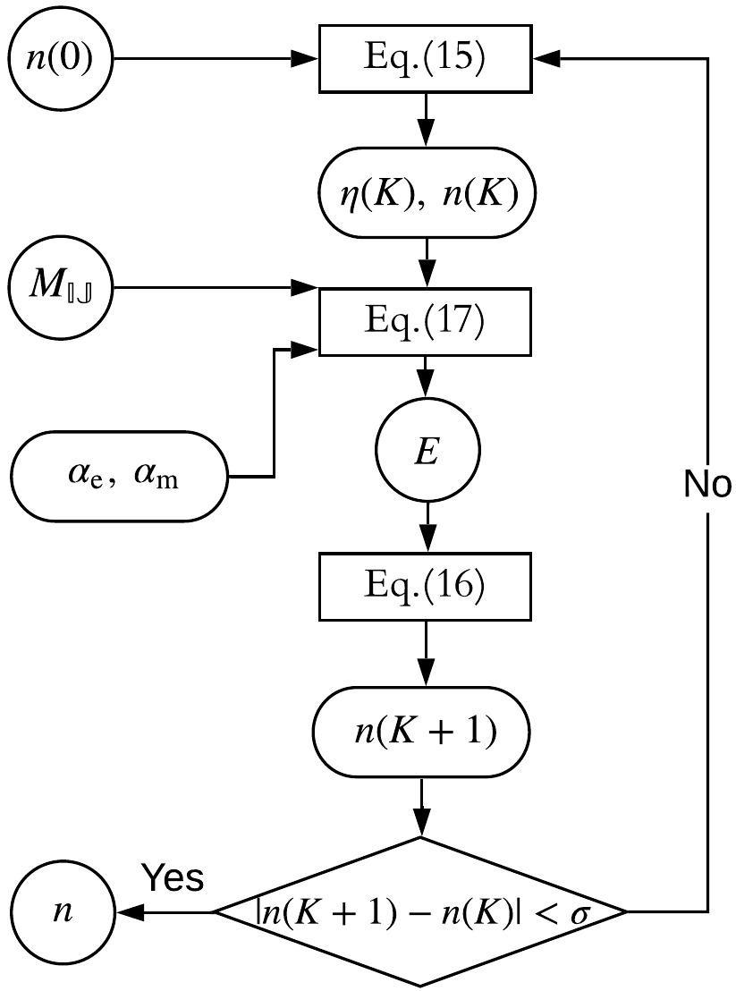
We propose an iterative algorithm for the calculation of $E$ and $n$. The electric field is calculated by Eq. (13a) with an initial guess of refractive index $n(0)$. Then a new refractive index $n(1)$ is calculated from the electric field by Eq. (16), and $n(1)$ is subsequently used in Eq. (13a) to again calculate the electric field. This process is repeated until we reach the convergence criterion in the $K$-th iteration, $|n(K)-n(K-1)|/|n(K-1)|<\sigma$. The user-defined value of $\sigma$ varies depending on specific applications, which is chosen to be $0.1\%$ in this paper. This is discussed in Fig. 3 and below.

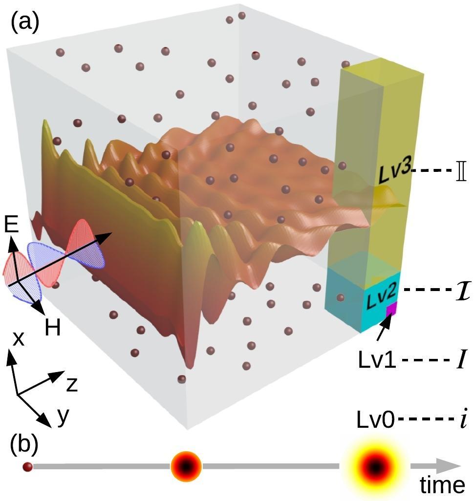
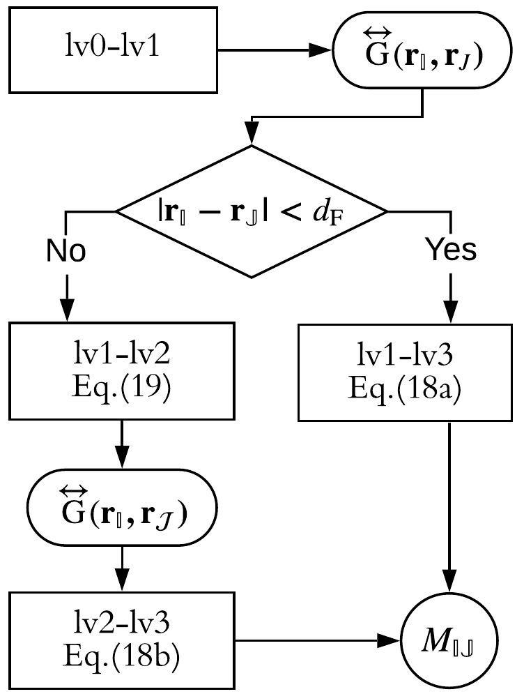
The analytic description of an infinite number of particles in a semi-infinite half-space given above provides a means for calculating the effective refractive index, however numerics must be carried out over a finite number of particles, and so we confine our attention to a finite-sized box as described below. The simulation region is taken to be a cube shown in Fig. 1(a). The $N$ particles are diffused into volumetric currents as described in Sec. II.2. The diffusion of a single particle is illustrated in Fig. 1(b). Although solving the interaction of $N$ particles is a challenge, the hierarchical clustering method, with the concept inspired by works in other research fields Song et al. 1997; Hackbusch 1999; Shih et al. 2006; Shih et al. 2007; Arkhipov et al. 2006; Arkhipov et al. 2008; Corpet 1988; Johnson 1967, reduces the computational complexity from $O(N^{3})$ to $O(N_{\rm top}^{3})$, where $N_{\rm top}$ is the number of top level structures. With a diagram given in Fig. 2, the calculations are performed in four levels: at Level 0 (lv0), fields scattered from individual particles are calculated; at Level 1 (lv1) particles are clustered into cubes with homogeneous permittivity and permeability such that the field scattered from that cube matches the field scattered from lv0 particles within a cube in a minimum $\ell_{2}$-norm error sense; at Level 2 (lv2), the cubes are clustered into larger cubes treated as homogeneous so the field scattered from a lv2 voxel is equivalent to the field scattered from all the lv1 voxels within the lv2 voxel; at Level 3 (lv3), the lv2 voxels are clustered into columns, which again are treated as homogeneous, and fields scattered from these columns are calculated. The side length of the lv2 voxel is equivalent to the cross-section side length of the lv3 column. The fields scattered by individual particles, that is the calculation at lv0, are described by Eq. (12). The lv1 and lv2 fields, those are fields scattered by the cubes, are given by Eq. (13a). The lv3 fields, those are fields scattered by the columns, are given by

Here $\Delta S_{\rm 2}=(\Delta L_{\rm 2})^{2}$ denotes the area of the lv3 column on the $yz$ plane, where $\Delta L_{\rm 2}$ is the side length of a lv2 voxel, and $M_{\mathbb{I}\mathbb{J}}$ represents the re-summed discretized Green’s function for scattering from column $\mathbb{J}$ to column $\mathbb{I}$ at lv3 of a clustering procedure. We assume that near the center of the simulation volume the field propagating in the medium is, to a good approximation, plane-wave-like, see Fig. 1(a). With this assumption and the medium being isotropic, only the $xx$ component of $M_{\mathbb{I},\mathbb{J}}$ needs to be calculated for the incident field polarized along $\hat{x}$ direction, as then the field propagating in the medium must also be polarized along $\hat{x}$ direction. Thus, we see the benefit of the clustering approach: a problem set in 3 spatial dimensions in Eq. (13a) is reduced to a problem set in 2 spatial dimensions in Eq. (17).

The calculation of $M_{\mathbb{I}\mathbb{J}}$ is carried out in 2 different ways, with the diagram given in Fig. 2. The choice of which technique to use depends on the distance $|{{\bf R}}|=|{{\bf r}}_{\mathbb{I}}-{{\bf r}}_{\mathbb{J}}|$. The limit between the near field, $|{{\bf R}}|\leq d_{\rm F}$, and far field, $|{{\bf R}}|>d_{\rm F}$, is denoted as $d_{\rm F}$. The value of $d_{\rm F}$ can be pre-calculated as described in Appendix C. In the near field region, where the fine mesh is required, the calculation of $M_{\mathbb{I}\mathbb{J}}$ takes the lv0-lv1-lv3 hierarchical clustering procedure, while in the far field region, where the coarse approach is applicable, lv0-lv1-lv2-lv3 clustering is used:

where

Here $J$, the index of a lv1 voxel, ranges over all possible values within the lv2 voxels labelled by the index $\mathcal{J}$, which runs over all possible values within the lv3 column labelled by $\mathbb{J}$. The volume of a lv1 voxel is given by $\Delta V_{\rm 1}=(\Delta L_{\rm 1})^{3}$, where $\Delta L_{\rm 1}$ is the side length of a lv1 voxel. Introducing the lv2 voxels reduces computational complexity by reducing the number of scatterers interacting with each other.

In order to calculate the effective refractive index from Eq. (16), we need to simulate the scattered field in a cubic volume large enough so that in a region near the center of a cube the field behaves as if it propagates in a semi-infinite medium. On the other hand, the numerical complexity scales as $L^{6}$ where $L$ is a cube length, given the same discretization of the simulation region, i.e., the size of the lv1 voxel. The size of the cubic simulation volume in Fig. 1 is selected to balance the accuracy and complexity of the calculation. By repeated numerical experimentation, we found that a cube with a size of $L=4.2\lambda$ on a side allows us to calculate the effective refractive index while running a reasonable time ($<1$ hours on a $2.3$ GHz Intel Core i5 CPU), where $\lambda$ is the wavelength of the field in free-space. The total number of particles is chosen to be $N=4\times 10^{10}$ which corresponds to the atomic density of silicon for $\lambda=221$ nm at a temperature of $300$ K and under a pressure of $1$ atm.

The size of lv1 and lv2 voxels is determined as follows. The scattered field arises from the interaction of particles and the propagating field. The rapid variation of the susceptibilities can be ignored while the size of the voxels should be of the scale of the variations of the propagating field. So the side length of a lv1 voxel should be much smaller than the wavelength of the field propagating in the medium (i.e., less than $0.01\lambda/n$). Here we specifically assign the side length of a lv1 voxel as $0.0015\lambda$. The side length of the lv2 voxel is chosen to be $0.03\lambda$, justified by Fig. 9 in Appendix D. Indeed, increasing the size of the lv2 voxel to include more lv1 voxel reduces complexity. However, the error of the lv1-lv2 clustering procedure, plotted in Fig. 9, also increases, because of the non-trivial higher order of the multipole components of the voxel Darve 2000; Engheta et al. 1992; Coifman et al. 1993. Thus the size of the lv2 voxel is limited for the purpose of the accuracy of the calculation. Given this size and the concentration chosen, each lv2 voxel comprises $14600$ particles. The $N_{\rm 2}=2.74\times 10^{6}$ lv2 voxels at locations specified by coordinates $y$ and $z$ are clustered into $N_{\rm 3}=1.96\times 10^{4}$ columns, each consisting of $140$ lv2 voxels. The interaction matrix elements between columns, $M_{\mathbb{I}\mathbb{J}}$ is calculated as shown in the flow chart, Fig. 2. Much like a Green’s function in free space, $M_{\mathbb{I}\mathbb{J}}$, depends only on geometry and wavelength in free space, not on the refractive index or impedance. With $M_{\mathbb{I}\mathbb{J}}$ pre-calculated for our chosen hierarchical clustering process ¹¹ 1 The operator $M$ is a Toeplitz matrix if hexahedron mesh is used in the simulation. Taking advantage of the fact that the elements are repeated saves both RAM and CPU time., the effective refractive index and the electric field distribution in the simulation region are calculated using the iteration scheme given in Fig. 3.

With a goal in mind to find a material with an effective refractive index with a real part of 2, we take the particles polarizabilities to be $\alpha_{\rm e}=(1.41\times 10^{-9}+1.31\times 10^{-10}i)\lambda^{3}\varepsilon_{\rm 0}$ and $\alpha_{\rm m}=(5.62\times 10^{-10}+1.78\times 10^{-11}i)\lambda^{3}\mu_{\rm 0}$, starting from these values of polarizabilities, we can calculate the effective refractive index and the electric field distribution throughout the simulation region. To start the iteration process, the initial guess of the refractive index is taken to be the same as the free-space, $n(0)=1$. The convergence criterion, $|n(K)-n(K-1)|/|n(K-1)|<0.1\%$, is met in the $9$th iteration, with the resultant refractive index $2.0+0.2i$. The simulated electric field in the last iteration is shown in the middle plane in Fig. 1. It may be observed that this electric field is a superposition of the ideal planewave to which we fit to calculate the index of refraction plus the deviations from that ideal field generated by the boundaries.

Though the electric field and the refractive index have been acquired, the validity of Eq. (16) used to calculate the refractive index must be checked post hoc. Fig. 4 shows the deviation from the ideal planewave used to fit the field and extract the index. We see that in the region used to calculate the refractive index the planewave dominates in the sense that $\langle|{\rm arg}(E^{\rm plane})-{\rm arg}(E^{\rm simu})|/{\rm arg}(E^{\rm plane})\rangle<0.1\%$, where the $\langle...\rangle$ denotes averaging throughout the rectangle. The error of calculating the refractive index with Eq. (16) is thus limited to less than $0.2\%$.

Having established self-consistency, let us here compare the results of our diffused particle method with well-known results from the Clausius-Mossotti relation Clausius 1879; Mossotti 1850; Lorenz 1869; Lorentz 1909; Thackray et al. 2014; Markel 2005, that is we hold the magnetic polarizability to be zero so that the usual Clausius-Mossotti relation applies. We apply procedures as described above. The particles are chosen to be lossy, with polarizability ${\rm Im}(\alpha_{\rm m})=0.1{\rm Re}(\eta_{\rm 0}^{2}\alpha_{\rm e})$. With $\alpha_{\rm m}=0$, the term proportional to the curl of magnetic currents in Eq. (12) vanishes. As may be seen in Fig. 5(a), the simulated permittivity agrees well with the theoretical result given by the Clausius-Mossotti relation,

Then the diffused particle method is used to calculate the effective refractive index of the medium comprising particles responding to both electric and magnetic field, with $\alpha_{\rm e}=(5.55\times 10^{-9}+5.55\times 10^{-10}i)\lambda^{3}\varepsilon_{\rm 0}$ and $\alpha_{\rm m}=(5.55\times 10^{-10}+5.55\times 10^{-11}i)\lambda^{3}\mu_{\rm 0}$. In this case, the generalized Clausius-Mossotti relation Wang et al. 2020 gives 2 different values of the effective refractive index, $n_{\rm+}$ and $n_{\rm-}$. The simulated refractive index in Fig. 5(b) converges to either predicted value depending on the initial guess $n(0)$. The relative difference between the theoretical refractive index and the simulated value is less than $0.2\%$.

References

- Wang et al. (2020) L. Wang, I. L. Rasskazov, and P. S. Carney, (2020).
- Kelly et al. (2003) K. L. Kelly, E. Coronado, L. L. Zhao, and G. C. Schatz, The Journal of Physical Chemistry B 107, 668 (2003).
- Jain et al. (2006a) P. K. Jain, K. S. Lee, I. H. El-Sayed, and M. A. El-Sayed, The Journal of Physical Chemistry B 110, 7238 (2006a).
- Jain et al. (2006b) P. K. Jain, S. Eustis, and M. A. El-Sayed, Journal of Physical Chemistry B 110, 18243 (2006b).
- Pérez-Juste et al. (2005) J. Pérez-Juste, I. Pastoriza-Santos, L. M. Liz-Marzán, and P. Mulvaney, Coordination Chemistry Reviews 249, 1870 (2005).
- Jin et al. (2003) R. Jin, Y. Charles Cao, E. Hao, G. S. Métraux, G. C. Schatz, and C. A. Mirkin, Nature 425, 487 (2003).
- Huang et al. (2009) X. Huang, S. Neretina, and M. A. El-Sayed, Advanced Materials 21, 4880 (2009).
- Chen et al. (2005) J. Chen, F. Saeki, B. J. Wiley, H. Cang, M. J. Cobb, Z.-Y. Li, L. Au, H. Zhang, M. B. Kimmey, Li, and Y. Xia, Nano Letters 5, 473 (2005).
- Myroshnychenko et al. (2008) V. Myroshnychenko, J. Rodríguez-Fernández, I. Pastoriza-Santos, A. M. Funston, C. Novo, P. Mulvaney, L. M. Liz-Marzán, and F. J. García de Abajo, Chemical Society Reviews 37, 1792 (2008).
- Hartland (2011) G. V. Hartland, Chemical Reviews 111, 3858 (2011).
- Rasskazov et al. (2016) I. L. Rasskazov, S. V. Karpov, G. Y. Panasyuk, and V. A. Markel, Journal of Applied Physics 119, 043101 (2016).
- Jain and El-Sayed (2008) P. K. Jain and M. A. El-Sayed, Nano Letters 8, 4347 (2008).
- Giannini et al. (2011) V. Giannini, A. I. Fernández-Domínguez, S. C. Heck, and S. A. Maier, Chemical reviews 111, 3888 (2011).
- Willets and Van Duyne (2007) K. A. Willets and R. P. Van Duyne, Annual Review of Physical Chemistry 58, 267 (2007).
- Stiles et al. (2008) P. L. Stiles, J. A. Dieringer, N. C. Shah, and R. P. Van Duyne, Annual Review of Analytical Chemistry 1, 601 (2008).
- Ghosh and Pal (2007) S. K. Ghosh and T. Pal, Chemical Reviews 107, 4797 (2007).
- Lee and El-Sayed (2006) K.-S. Lee and M. A. El-Sayed, The Journal of Physical Chemistry B 110, 19220 (2006).
- Noguez (2007) C. Noguez, The Journal of Physical Chemistry C 111, 3806 (2007).
- Jain et al. (2007) P. K. Jain, W. Huang, and M. A. El-Sayed, Nano Letters 7, 2080 (2007).
- Klar et al. (1998) T. Klar, M. Perner, S. Grosse, G. von Plessen, W. Spirkl, and J. Feldmann, Physical Review Letters 80, 4249 (1998).
- Wiley et al. (2006) B. J. Wiley, S. H. Im, Z.-Y. Li, J. McLellan, A. Siekkinen, and Y. Xia, Journal of Physical Chemistry B 110, 15666 (2006).
- Tian et al. (2002) Z.-Q. Tian, B. Ren, and D.-Y. Wu, The Journal of Physical Chemistry B 106, 9463 (2002).
- van Dijk et al. (2013) T. van Dijk, S. T. Sivapalan, B. M. DeVetter, T. K. Yang, M. V. Schulmerich, C. J. Murphy, R. Bhargava, and P. S. Carney, The Journal of Physical Chemistry Letters 4, 1193 (2013).
- Bond et al. (2013) T. C. Bond, S. J. Doherty, D. W. Fahey, P. M. Forster, T. Berntsen, B. J. Deangelo, M. G. Flanner, S. Ghan, B. Kärcher, D. Koch, S. Kinne, Y. Kondo, P. K. Quinn, M. C. Sarofim, M. G. Schultz, M. Schulz, C. Venkataraman, H. Zhang, S. Zhang, N. Bellouin, S. K. Guttikunda, P. K. Hopke, M. Z. Jacobson, J. W. Kaiser, Z. Klimont, U. Lohmann, J. P. Schwarz, D. Shindell, T. Storelvmo, S. G. Warren, and C. S. Zender, Journal of Geophysical Research Atmospheres 118, 5380 (2013).
- Dubovik et al. (2006) O. Dubovik, A. Sinyuk, T. Lapyonok, B. N. Holben, M. Mishchenko, P. Yang, T. F. Eck, H. Volten, O. Muñoz, B. Veihelmann, W. J. van der Zande, J.-F. Leon, M. Sorokin, and I. Slutsker, Journal of Geophysical Research 111, D11208 (2006).
- Dubovik et al. (2000) O. Dubovik, A. Smirnov, B. N. Holben, M. D. King, Y. J. Kaufman, T. F. Eck, and I. Slutsker, Journal of Geophysical Research: Atmospheres 105, 9791 (2000).
- Watson (2002) J. G. Watson, Journal of the Air & Waste Management Association 52, 628 (2002).
- Weingartner and Draine (2001) J. C. Weingartner and B. T. Draine, The Astrophysical Journal 548, 296 (2001).
- Waterman (1971) P. C. Waterman, Physical Review D 3, 825 (1971).
- Varadan (1980) V. V. Varadan, Acoustic, electromagnetic, and elastic wave scattering–focus on the T-matrix approach (Pergamon, 1980).
- Egel et al. (2017) A. Egel, L. Pattelli, G. Mazzamuto, D. S. Wiersma, and U. Lemmer, Journal of Quantitative Spectroscopy and Radiative Transfer 199, 103 (2017).
- Pattelli et al. (2018) L. Pattelli, A. Egel, U. Lemmer, and D. S. Wiersma, Optica 5, 1037 (2018).
- Draine and Goodman (1993) B. T. Draine and J. Goodman, The Astrophysical Journal 405, 685 (1993).
- Draine and Flatau (1994a) B. T. Draine and P. J. Flatau, Journal of the Optical Society of America A 11, 1491 (1994a).
- Yurkin and Hoekstra (2011) M. A. Yurkin and A. G. Hoekstra, Journal of Quantitative Spectroscopy and Radiative Transfer 112, 2234 (2011).
- Penttilä et al. (2021) A. Penttilä, J. Markkanen, T. Väisänen, J. Räbinä, M. A. Yurkin, and K. Muinonen, Journal of Quantitative Spectroscopy and Radiative Transfer 262, 107524 (2021).
- Song et al. (1997) J. M. Song, C. C. Lu, and W. C. Chew, IEEE Transactions on Antennas and Propagation 45, 1488 (1997).
- Hackbusch (1999) W. Hackbusch, Computing 108, 89 (1999).
- Koç and Chew (2001) S. Koç and W. Chew, Journal of Electromagnetic Waves and Applications 15, 1447 (2001).
- Järvenpää et al. (2013) S. Järvenpää, J. Markkanen, and P. Ylä-Oijala, IEEE Transactions on Antennas and Propagation 61, 4393 (2013).
- Yurkin and Hoekstra (2007) M. A. Yurkin and A. G. Hoekstra, Journal of Quantitative Spectroscopy and Radiative Transfer IX Conference on Electromagnetic and Light Scattering by Non-Spherical Particles, 106, 558 (2007).
- Mulholland et al. (1994) G. W. Mulholland, C. F. Bohren, and K. A. Fuller, Langmuir 10, 2533 (1994).
- Foldy (1945) L. L. Foldy, Physical Review 67, 107 (1945).
- Lax (1951) M. Lax, Reviews of Modern Physics 23, 287 (1951).
- Lax (1952) M. Lax, Physical Review 85, 621 (1952).
- de Vries et al. (1998) P. de Vries, D. V. van Coevorden, and A. Lagendijk, Reviews of Modern Physics 70, 447 (1998).
- Chew (1995) W. C. Chew, Waves and fields in inhomogeneous media, Vol. 522 (IEEE press New York, 1995).
- Sun and Chew (2009) L. E. Sun and W. C. Chew, Waves in Random and Complex Media 19, 162 (2009).
- Cui et al. (2019) X.-H. Cui, K. Ding, J.-W. Dong, and C. T. Chan, Physical Review B 100, 115412 (2019).
- Born and Wolf (2013) M. Born and E. Wolf, Principles of optics: electromagnetic theory of propagation, interference and diffraction of light (Elsevier, 2013).
- Einstein (1905) A. Einstein, Annalen der Physik 322, 549 (1905).
- Einstein (1956) A. Einstein, Investigations on the Theory of the Brownian Movement (Courier Corporation, 1956).
- Barrera et al. (1988) R. G. Barrera, G. Monsivais, and W. L. Mochán, Physical Review B 38, 5371 (1988).
- Mishchenko et al. (2006) M. I. Mishchenko, L. D. Travis, and A. A. Lacis, Multiple scattering of light by particles: radiative transfer and coherent backscattering (Cambridge University Press, 2006).
- Mackowski and Mishchenko (2013) D. W. Mackowski and M. I. Mishchenko, Journal of Quantitative Spectroscopy and Radiative Transfer 123, 103 (2013).
- Ishimaru (1977) A. Ishimaru, Proceedings of the IEEE 65, 1030 (1977).
- Van Bladel (1961) J. Van Bladel, IRE Transactions on Antennas and Propagation 9, 563 (1961).
- Shih et al. (2006) A. Y. Shih, A. Arkhipov, P. L. Freddolino, and K. Schulten, The Journal of Physical Chemistry B 110, 3674 (2006).
- Shih et al. (2007) A. Y. Shih, P. L. Freddolino, A. Arkhipov, and K. Schulten, Journal of structural biology 157, 579 (2007).
- Arkhipov et al. (2006) A. Arkhipov, P. L. Freddolino, and K. Schulten, Structure 14, 1767 (2006).
- Arkhipov et al. (2008) A. Arkhipov, Y. Yin, and K. Schulten, Biophysical journal 95, 2806 (2008).
- Corpet (1988) F. Corpet, Nucleic acids research 16, 10881 (1988).
- Johnson (1967) S. C. Johnson, Psychometrika 32, 241 (1967).
- Darve (2000) E. Darve, SIAM Journal on Numerical Analysis 38, 98 (2000).
- Engheta et al. (1992) N. Engheta, W. D. Murphy, V. Rokhlin, and M. S. Vassiliou, IEEE Transactions on Antennas and Propagation 40, 634 (1992).
- Coifman et al. (1993) R. Coifman, V. Rokhlin, and S. Wandzura, IEEE Antennas and Propagation magazine 35, 7 (1993).
- (67) The operator is a Toeplitz matrix if hexahedron mesh is used in the simulation. Taking advantage of the fact that the elements are repeated saves both RAM and CPU time.
- Clausius (1879) R. Clausius, The mechanical theory of heat (Macmillan, 1879).
- Mossotti (1850) O. F. Mossotti, Mem. Soc. Ital 14, 49 (1850).
- Lorenz (1869) L. Lorenz, Experimentale og theoretiske Undersøgelser: over Legmernes Brydningsforhold (Bianco Luno, 1869).
- Lorentz (1909) H. A. Lorentz, The Theory of Electrons and Its Applications to the Phenomena of Light and Radiant Heat: A Course of Lectures Delivered in Columbia University, New York, in March and April, 1906, Vol. 29 (Columbia University Press, 1909).
- Thackray et al. (2014) B. D. Thackray, V. G. Kravets, F. Schedin, G. Auton, P. A. Thomas, and A. N. Grigorenko, ACS Photonics 1, 1116 (2014).
- Markel (2005) V. A. Markel, Journal of Physics B: Atomic, Molecular and Optical Physics 38, L115 (2005).
- (74) “https://github.com/lwang111/Diffused-Particle-Method,” .
- Chew and Wang (1990) W. Chew and Y. Wang, IEEE Transactions on Medical Imaging 9, 218 (1990).
- Lewin (1947) L. Lewin, Journal of the Institution of Electrical Engineers - Part III: Radio and Communication Engineering 94, 65 (1947).
- Khizhniak (1957) N. A. Khizhniak, Soviet Physics-Technical Physics 27, 2006 (1957).
- Holloway et al. (2003) C. Holloway, E. Kuester, J. Baker-Jarvis, and P. Kabos, IEEE Transactions on Antennas and Propagation 51, 2596 (2003).
- Zhao et al. (2009) Q. Zhao, J. Zhou, F. Zhang, and D. Lippens, Materials Today 12, 60 (2009).
- Draine and Flatau (1994b) B. T. Draine and P. J. Flatau, Journal of the Optical Society of America A 11, 1491 (1994b).
- Markel (2016) V. A. Markel, Journal of the Optical Society of America A 33, 1244 (2016).
- Kane Yee (1966) Kane Yee, IEEE Transactions on Antennas and Propagation 14, 302 (1966).
- Correia and Jin (2004) D. Correia and J.-M. Jin, Microwave and Optical Technology Letters 40, 201 (2004).
- (84) The value is approximated (with one significant digit) with a diffusivity corresponding to the Brownian motion of air molecules dissolved in water and a diffusion time ns which is enough for the electromagnetic fields to reach to a stable distribution in the simulated medium with a wavelength of nm.
- (85) Much larger than the standard deviation of the Gaussian distribution of the particle diffusion .