Limiting probabilities of first order properties of
random sparse graphs and hypergraphs

Alberto Larrauri Thanks: Universitat Politècnica de Catalunya, Department of Computer Science. E-mail: llzalberto@hotmail.com. Supported by the European Research Council (ERC) under the European Union’s Horizon 2020 research and innovation programme (grant agreement ERC-2014-CoG 648276 AUTAR). Tobias Müller Thanks: University of Groningen, Department of Mathematics. E-mail: tobias.muller@rug.nl. Marc Noy Thanks: Universitat Politècnica de Catalunya, Department of Mathematics. E-mail: marc.noy@upc.edu. Supported by the Ministerio de Economía y Competitividad grant MTM2017-82166-P.

Abstract

Let $G_{n}$ be the binomial random graph $G(n,p=c/n)$ in the sparse regime, which as is well-known undergoes a phase transition at $c=1$ . Lynch (Random Structures Algorithms, 1992) showed that for every first order sentence $\phi$ , the limiting probability that $G_{n}$ satisfies $\phi$ as $n\to\infty$ exists, and moreover it is an analytic function of $c$ . In this paper we consider the closure $\overline{L_{c}}$ in $[0,1]$ of the set $L_{c}$ of all limiting probabilities of first order sentences in $G_{n}$ . We show that there exists a critical value $c_{0}\approx 0.93$ such that $\overline{L_{c}}=[0,1]$ when $c\geq c_{0}$ , whereas $\overline{L_{c}}$ misses at least one subinterval when $c<c_{0}$ . We extend these results to random $d$ -uniform sparse hypergraphs, where the probability of a hyperedge is given by $p=c/n^{d-1}$ .

1 Introduction

We consider properties of random graphs expressible in the first order (FO) language of graphs, which is first order logic together with an adjacency relation $E(x,y)$ assumed to be symmetric and antireflexive. Our model is the binomial random graph $G(n,p)$ with vertex set $\{1,\dots,n\}$ and in which every edge is present independently with probability $p$ . We focus on the so-called sparse regime $p=c/n$ with $c>0$ . It is well-known that $G(n,c/n)$ undergoes a phase transition at $c=1$ , corresponding to the emergence of the giant component [2]. The model studied in [2] was the uniform model $G(n,M)$ on graphs with $n$ vertices and $M$ edges. However, the results we need in this work can be translated into the $G(n,p)$ model with the relation $M=p\binom{n}{2}$ .

Our starting point is the following result by Lynch [9]. The notation $G\models\phi$ means that the graph $G$ satisfies the sentence $\phi$ . We recall that a sentence is a FO formula without free variables, thus expressing a graph property closed under isomorphism.

Theorem.

For each FO sentence $\phi$ , the following limit exists:

p_{c}(\phi)=\lim_{n\to\infty}\mathbf{P}\{G_{n}\models\phi\}.

Moreover, $p_{c}(\phi)$ is a combination of sums, products, exponentials and a set of constants $\Lambda_{c}$ , hence it is an analytic function of $c$ .

The previous result shows in a strong form that FO logic does not capture the phase transition (see also [13] for a discussion including monadic second order logic).

Instead of considering limiting probabilities of single sentences, in this paper we consider the set of all limiting probabilities

L_{c}=\{p_{c}(\phi)\colon\phi\hbox{ FO sentence}\},

and its topological closure $\overline{L_{c}}$ in $[0,1]$ . Our main result is that there is a transition in the structure of $\overline{L_{c}}$ at a particular value of $c$ . We say that $\overline{L_{c}}$ contains a gap if there is at least one subinterval $[a,b]\subseteq[0,1]$ with $a<b$ such that $\overline{L_{c}}\cap[a,b]=\emptyset$ .

Theorem 1.1.

Let $\overline{L_{c}}$ be the closure of the of limiting probabilities of first order sentences in $G(n,c/n)$ . Let $c_{0}\approx 0.93$ be the unique positive solution of

e^{\frac{c}{2}+\frac{c^{2}}{4}}\sqrt{1-c}=\frac{1}{2}.

(1)

Then for every $c>0$ the set $\overline{L_{c}}$ is a finite union of closed intervals. Moreover, the following holds:

1.

$\overline{L_{c}}=[0,1]$ for $c\geq c_{0}$ .
2.

$\overline{L_{c}}$ has at least one gap for $0<c<c_{0}$ .

Remark.

This line of research was considered in [4] for minor-closed classes of graphs under the uniform distribution. For instance, it was shown there that for the class of acyclic graphs (forests), the set $\overline{L_{c}}$ is the union of 4 disjoint intervals. It was also shown that for every minor-closed class of graphs whose forbidden minors are all 2-connected, $\overline{L_{c}}$ is always a finite union of at least two intervals.

We extend the previous result to random sparse hypergraphs. We consider the model $G^{d}(n,p)$ of random $d$ -uniform hypergraphs, where every $d$ -edge has probability $p$ of being in $G^{d}(n,p)$ independently. When $p=c/n^{d-1}$ the expected number of edges $p\binom{n}{d}$ is linear in $n$ , justifying the qualifier ‘sparse’. A phase transition also occurs in $G^{d}(n,c/n^{d-1})$ when $c=(d-2)!$ , as shown in [12].

Theorem 1.2.

Let $d\geq 3$ be fixed and let $\overline{L_{c}}$ be the closure of the of limiting probabilities of first order sentences in $G^{d}(n,c/n^{d-1})$ . Let $c_{0}$ be the unique positive solution of

\exp\left({\frac{c}{2(d-2)!}}\right)\sqrt{1-\frac{c}{2(d-2)!}}=\frac{1}{2}.

(2)

Then for every $c>0$ the set $\overline{L_{c}}$ is a finite union of intervals. Moreover, the following holds:

1.

$\overline{L_{c}}=[0,1]$ for $c\geq c_{0}$ .
2.

$\overline{L_{c}}$ has at least one gap for $0<c<c_{0}$ .

We remark that $c_{0}=r(d-2)!$ , where $r\approx 0.898$ is the positive solution of $\exp(r/2)\sqrt{(}1-r)=1/2$ . As we will see the difference between Equations (1) and (2) comes from the fact that in graphs we consider cycles of length at least 3, whereas in hypergraphs we have to consider cycles of length at least 2.

Here is a summary of the paper. In Section 2 we review several preliminaries we need on probability, random graphs and logic. In Section 3 we prove Theorem 1.1, and in Section 4 we prove Theorem 1.2. To avoid repetition the preliminary results needed for hypergraphs in Section 4 are only sketched.

2 Preliminaries

We start with Brun’s sieve for obtaining limiting Poisson distributions [see 1, Theorem 1.23].

Lemma 2.1.

Let $X_{n,1},\dots,X_{n,k}$ be non-negative integer valued random variables defined over the same probability space. Let $\lambda_{1},\dots,\lambda_{k}\in\mathbb{R}$ be non-negative. Suppose that given for $a_{1},\dots,a_{k}\geq 0$ it holds that

\lim\limits_{n\to\infty}\mathrm{E}\left[\prod_{i=1}^{k}\binom{X_{n,i}}{a_{i}}\right]=\prod_{i=1}^{k}\frac{\lambda_{i}^{a_{i}}}{a_{i}!}.

Then the $X_{n,i}$ converge in distribution to independent Poisson variables whose respective means are the $\lambda_{i}$ . That is, for any $b_{1},\dots,b_{k}\geq 0$

\lim\limits_{n\to\infty}\mathbf{P}\left(\bigwedge_{i=1}^{k}X_{n,i}=b_{i}\right)=\prod_{i=1}^{k}e^{-\lambda_{i}}\frac{\lambda_{i}^{b_{i}}}{b_{i}!}.

Next we present several results on the number of cycles in random sparse graphs. Let the number $X_{n,k}$ of $k$ -cycles in $G(n,c/n)$ . It is easy to show that

\mathrm{E}[X_{n,k}]\leq\frac{c^{k}}{2k},

and

\lim\limits_{n\to\infty}\mathrm{E}[X_{n,k}]=\frac{c^{k}}{2k}.

The first part of the next lemma appears already in [2] for the $G(n,M)$ model. The second part is easily proved using the method of moments [1, Theorem 1.23].

Lemma 2.2.

For fixed $k\geq 3$ , the number of $k$ -cycles $X_{n,k}$ in $G(n,c/n)$ is distributed asymptotically as $n\to\infty$ as a Poisson law with parameter $\lambda_{k}=\frac{c^{k}}{2k}$ . Moreover, for fixed $k$ the random variables $X_{n,3},\dots,X_{n,k}$ are asymptotically independent.

We set

f(c)=\frac{1}{2}\ln\frac{1}{1-c}-\frac{c}{2}-\frac{c^{2}}{4}.

(3)

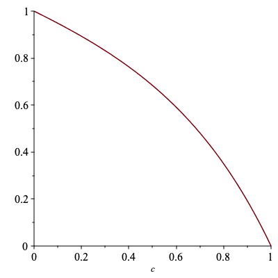
This is a function defined on $(0,1)$ that plays an important role in our results. The function is $e^{-f(c)}$ the limiting probability that $G(n,c/n)$ is acyclic; see Figure 1 for a plot.

Refer to caption — Figure 1: The probability that $G(n,c/n)$ has no cycles as a function of $c$ .

Corollary 2.3.

When $c<1$ the expected number of cycles in $G(n,c/n)$ is $f(c)$ .

Moreover, the limiting probability as $n\to\infty$ that $G(n,c/n)$ contains no cycle is

e^{-f(c)}=e^{\frac{c}{2}+\frac{c^{2}}{4}}\sqrt{1-c}.

Proof.

We have

\lim_{n\to\infty}\mathbf{E}\left[\sum_{k\geq 3}X_{n,k}\right]=\sum_{k\geq 3}\frac{c^{k}}{2k}=f(c).

The second statement follows from Lemma 2.2. ∎

A graph is unicyclic, or a unicycle, if it is connected and has a unique cycle. A unicyclic graph has a simple structure: it consists of a cycle of length at least 3 and a collection of rooted trees attached to its vertices. The size of a unicyclic graph is the number of edges, which is equal to the number of vertices (we use this convention because for hypergraphs it is more convenient to define size as the number of edges). We denote by $\mathcal{U}$ the family of unlabeled graphs whose connected components are all unicyclic, and we let $\mathcal{U}_{n}=\{H\in\mathcal{U}\,:\,|H|=n\}$ and $\mathcal{U}_{\leq n}=\bigcup_{i=1}^{n}\mathcal{U}_{i}$ .

The following is well-known; see [3, Lemma 2.10] for a proof in the $G(n,p)$ model. We say that a property holds asymptotically almost surely (a.a.s.) if it holds with probability tending to 1 as $n\to\infty$ .

Lemma 2.4.

Let $p(n)\sim c/n$ with $0<c<1$ . Then a.a.s all the connected component of $G(n,p)$ are either trees or unicycles.

Given a graph $G$ , we define its fragment $\mathrm{Frag}(G)$ as the union of all the unicyclic components in $G$ . We will write $\mathrm{Frag}_{n}$ to denote the fragment of $G(n,p)$ . The following result states that below the critical value $c=1$ the expected size of $\mathrm{Frag}_{n}$ is asymptotically bounded.

Lemma 2.5.

Let $p(n)\sim c/n$ with $0<c<1$ . Then $\lim\limits_{n\to\infty}\mathrm{E}[|\mathrm{Frag}_{n}|]$ exists and is a finite quantity.

Proof.

This is done in [2, Theorem 5d] for the uniform model and in greater detail in [3, Lemma 2.11] for the binomial model. For future reference we sketch the main ingredients in the proof.

Let $Y_{n,i}$ be the random variable equal to the number of unicyclic components in $G_{n}$ that contain exactly $i$ edges. Then one proves that for $k$ large enough and $n\geq 0$

\mathrm{E}[Y_{n,k}]\leq(ce^{1-c})^{k}e^{c/2}.

Furthermore, for all $k\geq 3$

\lim\limits_{n\to\infty}\mathrm{[}Y_{n,k}]=C(k,k)(ce^{-c})^{k},

where $C(k,k)$ denotes the number of labeled unicyclic graphs on $k$ vertices. Then the statement follows from the Dominated Convergence Theorem. ∎

Let $\phi$ be a first order sentence. We recall that the quantifier rank $\mathrm{qr}(\phi)$ is the maximum number of nested quantifiers in $\phi$ . It is shown in [9] that whether $G_{n}$ satisfies $\phi$ or not depends only a.a.s. on the induced unicycles in $G_{n}$ of diameter at most $3^{k}$ , where $k=\mathrm{qr}(\phi)$ (see Theorems 4.7, 4.8 and 4.9 in [9]). This, together with the fact that for $c<1$ a.a.s. the connected components of $G_{n}$ are either trees or unicycles (see Theorem 2.4), implies the following:

Lemma 2.6.

Let $p(n)\sim c/n$ with $0<c<1$ . Let $\phi$ be a FO sentence and let $H\in\mathcal{U}$ . Then

\lim\limits_{n\to\infty}\mathbf{P}\big(\,G(n,p)\models\phi\,\big|\,\mathrm{Frag}_{n}\simeq H\,\big)=\text{$0$ or $1$}.

Moreover, the value of the limit depends only on $\phi$ and $H$ , and not on $c$ .

Because of Lemma 2.4, when $0<c<1$ a.a.s. all cycles in $G_{n}$ are contained in unicyclic components. Since the expected number $f(c)$ of cycles in $G_{n}$ is asymptotically bounded we obtain the following.

Corollary 2.7.

Let $p(n)\sim c/n$ with $0<c<1$ , and let $Z_{n}$ be the random variable equal to the number of cycles in $G(n,p)$ that belong to connected components that are not trees or unicycles. Then

\lim\limits_{n\to\infty}\mathrm{E}[Z_{n}]=0.

Let $\mathrm{aut}(H)$ denote the number of automorphisms of a graph $H$ .

Lemma 2.8.

Let $p(n)\sim c/n$ with $c>0$ . Let $T$ be a finite set of unlabeled unicycles. For each $H\in T$ let $X_{n,H}$ be the random variable equal to the number of connected components in $G(n,p)$ isomorphic to $H$ , and let $\lambda_{H}=\frac{(e^{-c}c)^{|H|}}{\mathrm{aut}(H)}$ . Then

\lim\limits_{n\to\infty}\mathbf{P}\left(\bigwedge_{H\in T}X_{n,H}=a_{H}\right)=\prod_{H\in T}e^{-\lambda_{H}}\frac{\lambda_{H}^{a_{H}}}{a_{H}!}.

In other words, the $X_{n,H}$ converge in distribution to independent Poisson variables with respective means $\lambda_{H}$ .

Proof.

The proof is a slight modification of Theorem 4.8 in 1. It follows from a straightforward application of Theorem 2.1. ∎

We also need a classical result conjectured by Kakeya [6] and later proven in [10] on the set of subsums of a convergent series of non-negative terms.

Lemma 2.9.

Let $\sum_{n\geq 0}p_{n}$ be a convergent series of non-negative real numbers. Then the following are equivalent:

(1)

$p_{i}\leq\sum_{j>i}p_{j}$ for all $i\geq 0$ .
(2)

$\left\{\sum_{i\in A}p_{i}\colon A\subset\mathbb{N}\right\}=\left[0,\sum_{n=0}^{\infty}p_{n}\right].$

Moreover, if the condition $p_{i}\leq\sum_{j>i}p_{j}$ holds for all values of $i$ large enough, then the set $\left\{\sum_{i\in A}p_{i}\colon A\subset\mathbb{N}\right\}$ is a finite union of intervals.

3 Proof of Theorem 1.1

Before proceeding with the proof we outline the main components in the proof:

•

For $c\geq 1$ we can approximate any $p\in[0,1]$ with probabilities of statements of the form “there are at most $l$ cycles of length at most $k$ in $G(n,c/n)$ ” (Section 3.1).
•

We prove that the constant $c_{0}$ given by Equation 1 satisfies that $\overline{L_{c}}$ contains at least one gap whenever $c<c_{0}$ (Section 3.2).
•

For $c<1$ we show that

$\overline{L_{c}}=\left\{\sum_{H\in T}p_{H}(c)\colon T\subseteq\mathcal{U}\right\},$

where $p_{H}(c)=\lim\limits_{n\to\infty}\mathbf{P}\big(\mathrm{Frag}_{n}\simeq H\big)$ is given by Equation 5. In other words, $\overline{L_{c}}$ coincides with the set of subsums of the convergent series $\displaystyle\sum_{H\in\mathcal{U}}p_{H}(c)=1$ .
•

Using Kakeya’s Criterion (Lemma 2.9) we show that the set $\overline{L_{c}}$ of subsums of $\sum_{H\in\mathcal{U}}p_{H}(c)$ is always a finite union of intervals (Section 3.4).
•

Using Kakeya Criterion (Lemma 2.9) once again we prove that $\overline{L_{c}}$ is the whole interval $[0,1]$ for $c_{0}\leq c<1$ (Section 3.5).

3.1 No gap when $c\geq 1$

Let $X_{k}$ be as before the number of cycles of length $k$ in $G(n,c/n)$ , which is asymptotically $\hbox{Po}(c^{k}/(2k)$ ). Moreover, for fixed $k$ , the random variables $X_{3},\dots,X_{k}$ are asymptotically independent by Lemma 2.2. Hence for fixed $k$ ,

X_{\leq k}=X_{3}+\dots+X_{k}\xrightarrow[n\to\infty]{\text{d}}\hbox{Po}\left(\sum_{i=3}^{k}\frac{c^{k}}{2k}\right).

Since $c\geq 1$ the mean $\sum_{i=3}^{k}c^{k}/2k$ is not bounded as $k$ grows to infinity so we can pick $k$ such that this mean is as large as we like. Note that for any $k$ and $a$ the property that $X_{\leq k}\leq a$ can be expressed in FO logic. By the central limit theorem we have, for any fixed $x\in\mathbb{R}$

\mathbf{P}(\hbox{Po}(\mu)\leq\mu+x\sqrt{\mu})\xrightarrow[\mu\to\infty]{}\Phi(x),

where $\Phi(x)=\frac{1}{\sqrt{2\pi}}\int_{-\infty}^{x}e^{-t^{2}/2}dt$ is the c.d.f. of the standard normal law.

For $0<p<1$ and $\epsilon>0$ we can find $x$ such that $\Phi(x)=p$ , a value $\mu_{0}$ such that $\mathbf{P}(\mathrm{Po}(\mu)\leq\mu+x\sqrt{\mu})\in(p-\epsilon,p+\epsilon)$ for all $\mu\geq\mu_{0}$ , and then finally a $k$ such that $\sum_{i=3}^{k}\frac{c^{k}}{2k}\geq\mu_{0}$ . Hence there exists a FO property $\phi$ with limiting probability within $\epsilon$ of $p$ .

3.2 At least one gap when $c<c_{0}$

Let $e^{-f(c)}$ be as in Corollary 2.7 the limiting probability that $G_{n}=G(n,c/n)$ is acyclic. By elementary calculus $e^{-f(c)}$ is strictly decreasing for $c\in[0,1]$ (see Figure 1), and by definition of $c_{0}$ we have $e^{-f(c_{0})}=1/2$ .

Fix $c<c_{0}$ , and let $p(n)\sim c/n$ . We are going to show that $\overline{L_{c}}$ has a gap around $1/2$ . Let $A_{n}$ be the event that $G_{n}$ is acyclic and let $\phi$ be a FO sentence and let $p(\phi)=\lim\limits_{n\to\infty}\mathbf{P}\big(G_{n}\models\phi)$ . Then

	$\displaystyle p(\phi)$	$\displaystyle=\lim\limits_{n\to\infty}\mathbf{P}\big(G_{n}\models\phi\big\|A_{n}\big)\mathbf{P}(A_{n})+\mathbf{P}\Big(G_{n}\models\phi\big\|\neg A\Big)\mathbf{P}(\neg A_{n})$
		$\displaystyle=\lim\limits_{n\to\infty}\mathbf{P}\big(G_{n}\models\phi\,\big\|\,A_{n}\big)e^{-f(c)}+\mathbf{P}\big(G_{n}\models\phi\,\big\|\,A_{n}\big)(1-e^{-f(c)}).$		(4)

Because of Lemma 2.6 we have

\lim\limits_{n\to\infty}\mathbf{P}\big(G_{n}\models\phi\,\Big|\,A_{n}\big)=\text{$0$ or $1$}.

If the last limit equals 0 then from Equation 4 we obtain that $p(\phi)\leq 1-e^{-f(c)}$ . Otherwise, if the limit is 1, we have $p(\phi)\geq e^{-f(c)}$ . Since $e^{-f(c)}$ is strictly decreasing, $c<c_{0}$ and $e^{f(c_{0})}=1/2$ it follows that $e^{-f(c)}>1/2$ . As a consequence $1-e^{-f(c)}<1/2<e^{-f(c)}$ and $(1-e^{-f(c)},e^{-f(c)})$ is a gap of $\overline{L_{c}}$ .

3.3 Asymptotic distribution of the fragment for $c<1$ and its consequences

We compute below that the asymptotic probability that the fragment $\mathrm{Frag}_{n}$ is isomorphic to a given union $H$ of unicycles.

Lemma 3.1.

Let $p(n)\sim c/n$ with $0<c<1$ , and let $H\in\mathcal{U}$ . Then

\lim\limits_{n\to\infty}\mathbf{P}\big(\mathrm{Frag}_{n}\simeq H\big)=e^{-f(c)}\frac{(e^{-c}c)^{|H|}}{\mathrm{aut}(H)}.

(5)

Proof.

Fix such an $H$ . Let $U_{1},U_{2},\dots,U_{i},\dots$ be an enumeration of all unlabeled unicycles ordered by non-decreasing size. For each $i$ let $a_{i}$ be the number of connected components of $H$ that are copies of $U_{i}$ , and let $W_{n,i}$ be the random variable equal to the number of connected components in $G_{n}$ that are isomorphic to $U_{i}$ . Clearly $\mathrm{Frag}_{n}\simeq H$ if and only if $W_{n,i}=a_{i}$ for all $i$ . Thus,

\lim\limits_{n\to\infty}\mathbf{P}\big(\mathrm{Frag}_{n}\simeq H\big)=\lim\limits_{n\to\infty}\mathbf{P}\big(\bigwedge_{i=1}^{\infty}W_{n,i}=a_{i}\big).

First, we are going to show that

\lim\limits_{n\to\infty}\mathbf{P}\big(\bigwedge_{i=1}^{\infty}W_{n,i}=a_{i}\big)=\lim\limits_{j\to\infty}\lim\limits_{n\to\infty}\mathbf{P}\big(\bigwedge_{i=1}^{j}W_{n,i}=a_{i}\big).

(6)

Fix $\epsilon>0$ . For each $k$ let $X_{n,k}$ be the random variable that counts the unicyclic connected components of $G_{n}$ with exactly $k$ edges. By Lemma 2.5 we have that for some $k_{0}$

\lim\limits_{n\to\infty}\sum_{l=k_{0}}^{\infty}\mathrm{E}\big[X_{n,l}\big]\leq\epsilon.

Let $k_{1}$ be the maximum number of edges in a connected component of $H$ , and let $k=\max(k_{0},k_{1}+1)$ . Finally, fix $j_{0}$ such that $e(U_{j})>k_{1}$ for any $j\geq j_{0}$ . Let $j\geq j_{0}$ . Then $\mathrm{Frag}_{n}\simeq H$ if and only if

\bigwedge_{i=1}^{j}W_{n,i}=a_{i},\qquad\text{ and }\sum_{\ell=k}^{\infty}X_{n,l}=0.

Using Markov’s inequality we get

\lim\limits_{n\to\infty}\mathbf{P}\big(\sum_{\ell=k}^{\infty}X_{n,\ell}\geq 1\big)\leq\epsilon.

And in consequence,

\left|\lim\limits_{n\to\infty}\mathbf{P}\big(\bigwedge_{i=1}^{\infty}W_{n,i}=a_{i}\big)-\lim\limits_{j\to\infty}\lim\limits_{n\to\infty}\mathbf{P}\big(\bigwedge_{i=1}^{j}W_{n,i}=a_{i}\big)\right|\leq\epsilon,

proving eq. 6.

Using Lemma 2.8 we get

\lim\limits_{j\to\infty}\lim\limits_{n\to\infty}\mathbf{P}\big(\bigwedge_{i=1}^{j}W_{n,i}=a_{i}\big)=\prod_{i=1}^{\infty}e^{-\lambda_{i}}\frac{\lambda_{i}^{a_{i}}}{a_{i}!},

where $\lambda_{i}=\frac{(ce^{-c})^{|U_{i}|}}{\mathrm{aut}(U_{i})}=\lim\limits_{n\to\infty}\mathrm{E}[W_{n,i}]$ . Using Corollary 2.7 together with the dominated convergence theorem as in the proof of Lemma 2.5 we obtain

\sum_{i=1}^{\infty}\lambda_{i}=f(c),

and as a consequence

\prod_{i=1}^{\infty}e^{-\lambda_{i}}=e^{-f(c)}=e^{-f(c)}.

Since $\sum_{i=1}^{\infty}|U_{i}|a_{i}=|H|$ and $\prod_{i=1}^{\infty}\mathrm{aut}(U_{i})^{a_{i}}a_{i}!=\mathrm{aut}(H)$ , we finally get

\prod_{i=1}^{\infty}\frac{\lambda_{i}^{a_{i}}}{a_{i}!}=\frac{(ce^{-c})^{|H|}}{\mathrm{aut}(H)},

and the result follows. ∎

Given $H\in\mathcal{U}$ we define $p_{H}=p_{H}(c)=\lim\limits_{n\to\infty}\mathbf{P}\Big(\mathrm{Frag}_{n}\simeq H\Big)$ . The following is a direct consequence of the fact that the expected size of $\mathrm{Frag}_{n}$ is bounded.

Lemma 3.2.

Let $p(n)\sim c/n$ with $0<c<1$ , and let $\mathcal{T}\subset\mathcal{U}$ . Then

\lim\limits_{n\to\infty}\mathbf{P}\left(\bigvee_{H\in\mathcal{T}}\mathrm{Frag}_{n}\simeq H\right)=\sum_{H\in\mathcal{T}}p_{H}.

In particular, $\sum_{H\in\mathcal{T}}p_{H}=1$ .

Proof.

If $\mathcal{T}$ is finite then the statement is clearly true, since the events $\mathrm{Frag}_{n}\simeq H$ are disjoint for different $H$ . Suppose otherwise. Let $H_{1},\dots,H_{i},\dots$ be an enumeration of $\mathcal{T}$ by non-decreasing size. Fix $\epsilon>0$ . Let $m=\lim\limits_{n\to\infty}\mathrm{E}\big[|\mathrm{Frag}_{n}|\big]$ , and let $M=m/\epsilon$ . Then there exists $j_{0}$ such that $E(H_{j})\geq M$ for all $j\geq j_{0}$ . Using Markov’s inequality we obtain that for any $j\geq j_{0}$

		$\displaystyle\lim\limits_{n\to\infty}\left\|\mathbf{P}\left(\bigvee_{H\in T}\mathrm{Frag}_{n}\simeq H\right)-\sum_{i=1}^{j}p_{H_{i}}\right\|$
		$\displaystyle=\lim\limits_{n\to\infty}\left\|\mathbf{P}\left(\bigvee_{H\in T}\mathrm{Frag}_{n}\simeq H\right)-\mathbf{P}\left(\sum_{i=1}^{j}\mathrm{Frag}_{n}\simeq H\right)\right\|$
		$\displaystyle\leq\lim\limits_{n\to\infty}\mathbf{P}\Big(\|\mathrm{Frag}_{n}\|>M\Big)\leq\epsilon.$

As our choice of $\epsilon$ was arbitrary this proves the statement. ∎

We define $S_{c}$ as the set of subsums of $\sum_{H\in\mathcal{U}}p_{H}(c)$ ,

S_{c}:=\Big\{\sum_{H\in\mathcal{T}}p_{H}(c)\colon\mathcal{T}\subseteq\mathcal{U}\Big\}.

Theorem 3.3.

Let $0<c<1$ . Then $\overline{L_{c}}=S_{c}$ .

Proof.

We first show that $\overline{L_{c}}\subseteq S_{c}$ . It is a known fact [6], [5], [10] that $S_{c}$ is a perfect set, in particular $S_{c}$ is closed and $\overline{S_{c}}=S_{c}$ . Thus it is enough to show that $L_{c}\subset S_{c}$ .

Fix a FO property $P$ . We want to prove that $\lim\limits_{n\to\infty}\mathbf{P}(P(G_{n}))$ lies in $S_{c}$ . That is, we want to show that for some $\mathcal{T}\subseteq\mathcal{U}$

\lim\limits_{n\to\infty}\mathbf{P}\big(P(G_{n})\big)=\sum_{H\in\mathcal{T}}p_{H}.

(7)

Let $H\in\mathcal{U}$ . First we will prove that

\lim\limits_{n\to\infty}\mathbf{P}\big(P(G_{n})\big)=\sum_{H\in\mathcal{U}}\lim\limits_{n\to\infty}\mathbf{P}\big(\mathrm{Frag}_{n}\simeq H\big)\mathbf{P}\big(P(G_{n}))\,|\,\mathrm{Frag}_{n}\simeq H\big).

(8)

Let $H_{1},\dots,H_{i},\dots$ be an enumeration of $\mathcal{U}$ . Fix an arbitrarily small real constant $\epsilon>0$ . Notice that the events of the form $F_{n}\simeq H_{i}$ are disjoint for each $i$ . So we obtain:

\lim\limits_{n\to\infty}\mathbf{P}\big(P(G_{n})\big)=\lim\limits_{n\to\infty}\sum_{i=1}^{\infty}\big(\mathrm{Frag}_{n}\simeq H_{i}\big)\mathbf{P}\big(P(G_{n})\,|\,\mathrm{Frag}_{n}\simeq H_{i}\big).

Let $m=\lim\limits_{n\to\infty}\mathrm{E}\big[|\mathrm{Frag}_{n}|\big]$ and let $M=m/\epsilon$ . There exists some $j_{0}\in\mathbb{N}$ such that $|H_{i}|\geq M$ for all $i\geq j_{0}$ . As a consequence, for all $j\geq j_{0}$ ,

\lim\limits_{n\to\infty}\sum_{i=j}^{\infty}\mathbf{P}\big(\mathrm{Frag}_{n}\simeq H_{i}\big)\leq\epsilon.

And we obtain

	$\displaystyle\big\|\lim\limits_{n\to\infty}\mathbf{P}\big(P(G_{n})\big)-\sum_{i=1}^{j}\lim\limits_{n\to\infty}\mathbf{P}\big(\mathrm{Frag}_{n}\simeq H_{i}\big)\mathbf{P}\big(P(G_{n})\,\|\,\mathrm{Frag}_{n}\simeq H_{i}\big)\big\|$
	$\displaystyle=\lim\limits_{n\to\infty}\sum_{i=j}^{\infty}\mathbf{P}\big(\mathrm{Frag}_{n}\simeq H_{i}\big)\leq\epsilon$	.

This proves Equation 8. Because of Lemma 2.6 for all $H\in\mathcal{U}$

\lim\limits_{n\to\infty}\mathbf{P}\big(P(G_{n})\,|\,\mathrm{Frag}_{n}\simeq H\big)=0\text{ or }1.

Let $T=\{i\in\mathbb{N}\,|\,\lim\limits_{n\to\infty}\mathbf{P}\big(P(G_{n})\,|\,\mathrm{Frag}_{n}\simeq H_{i}\big)=1\,\}$ . Using Equation 8 we obtain

\displaystyle\sum_{i=1}^{\infty}\lim\limits_{n\to\infty}\mathbf{P}\big(\mathrm{Frag}_{n}\simeq H_{i}\big)\mathbf{P}\big(P(G_{n})\,|\,\mathrm{Frag}_{n}\simeq H_{i}\big)=\sum_{i\in T}p_{H_{i}}.

(9)

This proves Equation 7 and as a consequence $\overline{L_{c}}\subset S_{c}$ .

Now we proceed to prove $S_{c}\subset\overline{L_{c}}$ . Let $T\subset\mathcal{U}$ , and let $\epsilon>0$ be an arbitrarily small real number. We will show that there exists a FO property $P$ such that

\left|\lim\limits_{n\to\infty}\mathbf{P}\big(P(G_{n})\big)-\sum_{H\in T}p_{H}\right|\leq\epsilon.

(10)

First, notice that because of Lemma 3.2,

\sum_{H\in T}p_{H}=\lim\limits_{n\to\infty}\mathbf{P}\left(\bigvee_{H\in T}p_{H}\right).

We define the property $Q$ in the following way

Q(G):=\bigvee_{H\in T}\mathrm{Frag}(G)\sim H.

Let $m:=\lim\limits_{n\to\infty}\mathrm{E}\big[|\mathrm{Frag}_{n}|\big]$ , and let $M=2m/\epsilon$ . Then using Markov’s inequality:

\lim\limits_{n\to\infty}\mathbf{P}\big(\mathrm{Frag}_{n}\in\mathcal{U}_{\leq M}\big)\geq 1-\epsilon/2.

(11)

Also, using that $\mathrm{Frag}_{n}\neq\mathrm{Frag}_{n}^{M}$ implies that $|\mathrm{Frag}_{n}|\geq M$ ,

\lim\limits_{n\to\infty}\mathbf{P}\big(\mathrm{Frag}_{n}\neq\mathrm{Frag}^{M}_{n}\big)\leq\mathbf{P}\big(\mathrm{Frag}_{n}\in\mathcal{U}_{\leq M}\big)\leq\epsilon/2.

(12)

Let $T^{\prime}=T\cap\mathcal{U}_{\leq M}$ . As $\mathcal{U}_{\leq M}$ is a finite set so is $T^{\prime}$ . Define the properties $Q^{\prime}$ and $P$ as

Q^{\prime}(G)=\bigvee_{H\in T^{\prime}}\mathrm{Frag}(G)\sim H,\quad\text{ and }P(G)=\bigvee_{H\in T^{\prime}}\mathrm{Frag}^{M}(G)\sim H.

Notice that $P$ can be expressed in FO logic. Also, the implications $Q^{\prime}\implies Q$ and $Q^{\prime}\implies P$ hold. If $Q(G)$ holds and $\neg Q^{\prime}(G)$ holds as well then in particular $|\mathrm{Frag}(G)|\geq M$ . The same happens if $P(G)$ and $\neg Q^{\prime}(G)$ hold at the same time. Joining everything we get

		$\displaystyle\left\|\lim\limits_{n\to\infty}\mathbf{P}\big(P(G_{n})\big)-\sum_{H\in T}p_{H}\right\|=\left\|\lim\limits_{n\to\infty}\mathbf{P}\big(P(G_{n})\big)-\lim\limits_{n\to\infty}\mathbf{P}\big(Q(G_{n})\big)\right\|$
		$\displaystyle\leq\left\|\lim\limits_{n\to\infty}\mathbf{P}\big(P(G_{n})\big)-\lim\limits_{n\to\infty}\mathbf{P}\big(Q^{\prime}(G_{n})\big)\right\|+\left\|\lim\limits_{n\to\infty}\mathbf{P}\big(Q^{\prime}(G_{n})\big)-\lim\limits_{n\to\infty}\mathbf{P}\big(Q(G_{n})\big)\right\|$
		$\displaystyle\leq 2\mathbf{P}\big(\|\mathrm{Frag}_{n}\|\geq M\big)\leq\epsilon.$

∎

3.4 $\overline{L_{c}}$ is always a finite union of intervals

Since we have shown that there is no gap for $c\geq 1$ we only need to consider $c<1$ . Let $H_{1},\dots,H_{n},\dots$ be an enumeration of $\mathcal{U}$ such that $p_{H_{i}}(c)\leq p_{H_{j}}(c)$ for all $i\leq j$ . We shorten $p_{H_{i}}$ to $p_{i}$ . Because of Lemma 2.9 proving that $\overline{L_{c}}$ is a finite union of intervals amounts to showing that for all $i$ large enough

p_{i}\leq\sum_{j>i}^{\infty}p_{j}.

(13)

Let $f=f(c)$ be as defined in Equation 3, and let $s=ce^{-c}$ , and notice that as $c<1$ we have $s<1$ as well. We can rewrite the $p_{i}$ given by Equation 5 as

p_{i}=e^{-f}\frac{s^{|H_{i}|}}{aut(H_{i})}.

For $i\geq 1$ let $k(i)$ be the least integer such that

e^{-f}s^{k(i)-1}\geq p_{i}>e^{-f}s^{k(i)}.

Notice if $k\geq k(i)$ and $H_{j}\in\mathcal{U}_{k}$ then $p_{j}<e^{-f}s^{k}<p_{i}$ because $\mathrm{aut}(H_{j})\geq 1$ . For the same reason we also obtain that $|H_{i}|\leq k(i)-1$ . Hence to prove (13) it is sufficient to show that

p_{i}\leq\sum_{k\geq k(i)}\sum_{H_{j}\in\mathcal{U}_{k}}p_{j}.

(14)

Let $C_{x,y}$ denote the graph in $\mathcal{U}$ consisting of a cycle of length $x$ with a path of length $y$ attached to one of its vertices.If $y=0$ then $\mathrm{aut}(C_{x,y})=2x$ , and $\mathrm{aut}(C_{x,y})=2$ otherwise. Let $T_{x,y,z}$ be the graph consisting of a triangle with paths of length $x$ , $y$ , and $z$ attached to its three vertices. Note that $\text{aut}(T_{x,y,z})=1$ if $x,y,z$ are distinct, $\text{aut}(T_{x,y,z})=6$ if $x=y=z$ , and $\text{aut}(T_{x,y,z})=2$ otherwise. It is easy to see that $C_{3,k-3},C_{4,k-4},\dots,C_{k-1,1}$ together with $T_{0,1,k-4},T_{0,2,k-5},\dots,T_{0,\lfloor(k-3)/2\rfloor,\lceil(k-3)/2\rceil}$ form a family of different elements of $\mathcal{U}_{k}$ . We have that for $k\geq 3$

\sum_{i=3}^{k-1}p_{C_{i,k-i}}=e^{-f}s^{k}\frac{k-3}{2}.

If $k$ is odd $T_{0,\lfloor(k-3)/2\rfloor,\lceil(k-3)/2\rceil}$ has two automorphisms, and the remaining $T_{i,k-3-i}$ with $i\geq 1$ each have only one automorphism. If $k$ is even then all of $T_{0,1,k-4},T_{0,2,k-5},\dots,T_{0,\lfloor(k-3)/2\rfloor,\lceil(k-3)/2\rceil}$ have exactly one automorphism. This gives

\sum_{i=1}^{\lfloor(k-3)/2\rfloor}p_{T_{0,i,k-3-i}}=e^{-f}s^{k}\frac{k-4}{2},\quad\text{ for $k\geq 4$ }.

Using the last two equations it follows that for $k\geq 4$

\sum_{H\in\mathcal{U}_{k}}\frac{1}{\text{aut}(H)}\geq e^{-f}s^{k}\frac{2k-7}{2}.

(15)

Hence if $i$ is such that $(2k(i)-7)/2>1/s$ (that is, $k(i)>1/s+7/2$ ) then

\sum_{j>i}p_{j}\geq\sum_{H_{j}\in\mathcal{U}_{k(i)}}p_{j}\geq e^{-f}s^{k(i)}\frac{2k-7}{2}>e^{-f}s^{k(i)-1}\geq p_{i}.

Note that $k(i)>1/s+7/2$ whenever $|H_{i}|+1\geq 1/s+7/2$ , and this is true for sufficiently large $i$ .We have seen that, for any $0<c<1$ , it is indeed the case that $p_{i}<\sum_{j>i}p_{j}$ for all sufficiently large $i$ , as was to be proved.

3.5 No gap when $c_{0}\leq c<1$

Fix $c\in[c_{0},1)$ . Notice that in this case then $s=ce^{-c}$ satisfies

\frac{1}{3}<s<\frac{1}{e}.

Let $i$ be such that $k(i)\geq 4$ . Then, using (15) we obtain

\sum_{j>i}p_{j}\geq\sum_{k\geq k(i)}\sum_{H_{j}\in\mathcal{U}_{k}}p_{j}\geq\sum_{k\geq k(i)}e^{-f}s^{k}\frac{2k-7}{2}.

And using $\sum_{k=0}^{\infty}a^{k}(b+ck)=\frac{b}{1-a}+\frac{ca}{(1-a)^{2}}$ together with $s>1/3$ we obtain that

\sum_{j>i}p_{j}\geq e^{-f}s^{k(i)}\left(\frac{2k(i)-7}{2(1-s)}+\frac{s}{(1-s)^{2}}\right)\geq e^{-f}s^{k(i)}\frac{3k(i)-9}{2}.

In particular, since $\frac{3k-9}{2}\geq 3>1/s$ for all $k\geq 5$ , if $p_{i}\leq s^{4}$ then $p_{i}<\sum_{j>i}p_{j}$ . As a consequence, if $|H_{i}|\geq 4$ then $p_{i}<\sum_{j>i}p_{j}$ .

The only two cases left to consider are the ones when $H_{i}$ is either the empty graph or the triangle. If $H_{i}$ is the empty graph then necessarily $i=1$ because the empty graph is the most likely fragment. By the definition of $p_{0}$ critically we have $p_{1}\leq 1/2$ if $c\geq c_{0}$ , hence $p_{1}\leq\sum_{j>1}p_{j}$ . If $H_{i}$ is the triangle graph, then $p_{i}=e^{-f}s^{3}/6$ and

\displaystyle\sum_{j>i}p_{j}=\sum_{k\geq 4}\sum_{H_{j}\in\mathcal{U}_{k}}p_{j}

\displaystyle\geq\sum_{k\geq 4}e^{-f}s^{k}\frac{2k-7}{2}\geq e^{-f}s^{4}\frac{3}{2}\geq e^{-f}s^{3}\frac{1}{6}=p_{i},

as needed.

Thus $p_{i}\leq\sum_{j>i}p_{j}$ for every $i$ , as we needed to prove.

4 Proof of Theorem 1.2

Recall that we consider the model $G^{d}_{n}=G^{d}(n,p=c/n^{d-1})$ of random $d$ -uniform hypergraphs where each $d$ -edge has probability $p=c/n^{d-1}$ of being in $G^{d}_{n}$ independently, with $c>0$ . Throughout this section we consider $d\geq 3$ as being fixed and we will refer to “ $d$ -uniform hypergraphs” simply as hypergraphs. The FO language of $d$ -uniform hypergraphs is the FO language with a $d$ -ary relation which is anti-reflexive and completely symmetric. Analogously to the case of graphs, this relation symbolizes the adjacency relation in the context of $d$ -uniform hypergraphs.

The following is an analog of Lynch’s convergence law for random hypergraphs and can be found in [11, Proposition 6.4] and in more detail for more general relational structures in [8].

Theorem.

Let $p(n)\sim c/n^{d-1}$ . Then for each FO sentence $\phi$ , the following limit exists:

p_{c}(\phi)=\lim_{n\to\infty}\mathbf{P}\big(G^{d}_{n}\models\phi\big).

Moreover, $p_{c}(\phi)$ is a combination of sums, products, exponentials and a set of constants $\Lambda_{c}$ , hence it is an analytic function of $c$ .

As before we consider the set

L_{c}=\left\{\lim\limits_{n\to\infty}\mathbf{P}(G_{n}^{d}\models\phi)\,:\,\text{ $\phi$ FO sentence, and }p(n)\sim c/n^{d-1}\right\}.

4.1 Hypergraph preliminaries

Given a hypergraph $H$ , we denote the set of vertices by $V(H)$ and the set of edges by $E(H)$ . As in [7] we define the excess $\mathrm{ex}(H)$ of $H$ as the quantity

\mathrm{ex}(H)=(d-1)|H|-|V(H)|.

It is easily seen that the minimum excess of a connected hypergraph is $-1$ . A tree $T$ is a connected hypergraph satisfying $\mathrm{ex}(T)=-1$ . Equivalently, a tree is a hypergraph that can be obtained gluing edges repeatedly to an initial vertex in such a way that each new edge intersects the hypergraph obtained so far in exactly one vertex. A unicycle is a connected hypergraph of excess 0, and a cycle is a minimal unicycle. Equivalently a cycle is a connected hypergraph $H$ where every edge shares exactly two vertices with the remaining edges, and a unicycle is a cycle with disjoint trees attached to each vertex. A $k$ -cycle is a cycle with $k$ edges.

It is shown in [12] that a phase transition in the structure of $G_{n}^{d}$ occurs when $c=(d-2)!$ , similar to the one for random graphs. In particular, we have the following results [12, Theorem 3.6].

Lemma 4.1.

Let $p(n)\sim c/n^{d-1}$ with $0<c<(d-2)!$ . Then a.a.s. all connected components of $G^{d}_{n}$ are either trees or unicycles.

The proofs of the next results are very similar to those for graphs presented in Section 2 and are omitted.

Lemma 4.2.

Let $p\sim c/n^{d-1}$ with $c>0$ . For each $k\geq 2$ , let $X_{n,k}$ be the random variable equal to the number of $k$ -cycles in $G^{d}_{n}$ , and let $\lambda_{k}=\left(\frac{c}{(d-2)!}\right)^{k}$ . Then for fixed $k\geq 2$

(1)

$\mathrm{E}\big[X_{n,k}\big]\leq\lambda_{k}$ ,
(2)

$\lim\limits_{n\to\infty}\mathrm{E}\big[X_{n,k}\big]=\lambda_{k}$ ,
(3)

$X_{n,k}$ converges in distribution to a Poisson variable with mean $\lambda_{k}$ as $n\to\infty$ .

Furthermore, for any fixed $k\geq 2$ the variables $X_{n,2},\dots,X_{n,k}$ are asymptotically independent.

Corollary 4.3.

Let $p\sim c/n^{d-1}$ with $c>0$ . Set

f(c)=\sum_{k\geq 2}\left(\frac{c}{(d-2)!}\right)^{k}\frac{1}{2k}=\frac{1}{2}\ln\frac{1}{1-\frac{c}{(d-2)!}}-\frac{c}{2(d-2)!}.

(16)

Let $X_{n}$ be the random variable equal to the total number of cycles in $G^{d}_{n}$ . Then

\lim\limits_{n\to\infty}\mathrm{E}[X_{n}]=f(c),

and

\lim\limits_{n\to\infty}\mathbf{P}\Big(G^{d}_{n}\hbox{ contains no cycles}\Big)=e^{-f(c)}=\exp\left(\frac{c}{2(d-2)!}\right)\sqrt{1-\frac{c}{2(d-2)!}}.

Lemma 4.4.

Let $p\sim c/n^{d-1}$ with $0<c<(d-2)!$ . Let $Z_{n}$ be the random variable equal to the number of cycles in $G^{d}_{n}$ that belong to connected components that are not unicycles. Then

\lim\limits_{n\to\infty}\mathrm{E}[Z_{n}]=0.

Let $\mathcal{U}$ be the family of unlabeled $d$ -hypergraphs whose connected components are unicyclic.

Lemma 4.5.

Let $p\sim c/n^{d-1}$ with $c>0$ . Let $\mathcal{T}\subset\mathcal{U}$ be a finite set of unicycles. For each $H\in\mathcal{T}$ let $X_{n,H}$ be the random variable that counts the connected components in $G^{d}_{n}$ that are isomorphic to $H$ , and set

\lambda_{H}=\frac{\left(ce^{-c/(d-2)!}\right)^{|H|}}{aut(H)}.

Then $X_{n,H}$ converges in distribution to a Poisson variable with mean $\lambda_{H}$ as $n\to\infty$ and the $X_{n,H}$ are asymptotically independent, that is

\lim\limits_{n\to\infty}\mathbf{P}\left(\bigwedge_{H\in\mathcal{T}}X_{n,H}=a_{H}\right)=\prod_{H\in T}e^{-\lambda_{H}}\frac{\lambda_{H}^{a_{H}}}{a_{H}!}.

Define the fragment of hypergraph as the collection of components that are unicycles and let $\mathrm{Frag}_{n}$ be the fragment of the random hypergraph $G_{n}^{d}$ .

Lemma 4.6.

Let $p\sim c/n^{d-1}$ with $0<c<(d-2)!$ . Then the limit

\lim\limits_{n\to\infty}\mathrm{E}\big[|\mathrm{Frag}_{n}|\big]

exists and is a finite quantity.

Lemma 4.7.

Let $p\sim c/n^{d-1}$ with $0<c<(d-2)!$ . Let $\phi$ be a FO sentence and let $H\in\mathcal{U}$ . Then

\lim\limits_{n\to\infty}\mathbf{P}\Big(G^{d}_{n}\models\phi\,\Big|\,\mathrm{Frag}_{n}\simeq H\Big)=\text{ $0$ or $1$.}

Moreover, the value of the limit depends only on $\phi$ and $H$ , and not on $c$ .

As for graphs, we divide the proof of Theorem 1.2 into several cases. Along the way we analyze the distribution of the fragment and the number of automorphisms in hypergraphs.

4.2 No gap when $c\geq(d-2)!$

The arguments here mirror exactly those in Section 3.1. For each $k$ let $X_{n,k}$ be the random variable equal to the number of $k$ -cycles in $G^{d}_{n}$ . Then

X_{n,\leq k}=X_{n,2}+\dots+X_{n,k}\xrightarrow[n\to\infty]{\text{d}}\hbox{Po}\left(\sum_{i=2}^{k}\frac{(c/(d-2)!)^{k}}{2k}\right).

If $c\geq(d-2)!$ then $\sum_{i=2}^{k}\frac{(c/(d-2)!)^{k}}{2k}$ tends to infinity and we can use the Central Limit Theorem to approximate any $p\in(0,1)$ with FO statements of the form “ $X_{n,\leq k}\leq a$ ”.

4.3 At least when gap for $c<c_{0}$

Let $f(c)$ be as in Equation 16, and let $c_{0}$ be the unique solution of $e^{-f(c)}=1/2$ lying in $[0,(d-2)!]$ . Because of Corollary 4.3, $c_{0}$ is the only value for which

\lim\limits_{n\to\infty}\mathbf{P}\big(G^{d}_{n}\big)=1/2,

where $p(n)\sim c/n^{d-1}$ . One can check that this is achieved when the expected degree $c/(d-2)!$ is $\simeq 0.898$ , independently of $d$ .

Let $p(n)\sim c/n^{d-2}$ with $0<c<c_{0}$ . Because of Lemma 4.7, for any FO sentence $\phi$

\lim\limits_{n\to\infty}\mathbf{P}\big(G^{d}_{n}\models\phi\,\Big|\text{ $G^{d}_{n}$ contains no cycles }\big)=\text{ $0$ or $1$.}

From this point we continue as in Section 3.2 to show that $[1-e^{-f(c)},e^{-f(c)}]$ is a gap of $\overline{L_{c}}$ .

4.4 Asymptotic distribution of the fragment for $c<(d-2)!$

The same proof of Lemma 3.1 can be used to prove the following result.

Theorem 4.8.

Let $p(n)\sim c/n^{d-1}$ with $0<c<(d-2)!$ . Let $H\in\mathcal{U}$ . Then

\lim\limits_{n\to\infty}\mathbf{P}\big(\mathrm{Frag}_{n}\simeq H\big)=e^{-f(c)}\frac{\left(e^{-c/(d-2)!}c\right)^{|H|}}{aut(H)}.

For each $H\in\mathcal{U}$ define $p_{H}(c)=p_{H}=\lim\limits_{n\to\infty}\mathbf{P}\Big(\mathrm{Frag}_{n}\simeq H\Big)$ . Consider the set

S_{c}=\left\{\sum_{H\in\mathcal{T}}p_{H}(c)\,:\,\mathcal{T}\subseteq\mathcal{U}\right\}.

One can proceed exactly as in Theorem 3.3 to prove the following:

Theorem 4.9.

Let $0<c<(d-2)!$ . Then $\overline{L_{c}}=S_{c}$ .

4.5 A lower bound on the number of automorphisms of unicyclic hypergraphs

Let $H$ be an hypergraph and $h\in E(H)$ an edge. We call a vertex $v$ lying in $e$ free if $e$ is the only edge that contains $v$ . We denote by $\mathrm{free}(h)$ the number of free vertices in $e$ . Notice that

\mathrm{aut}(H)\geq\prod_{h\in E(H)}\mathrm{free}(h)!,

because free vertices inside an edge can be permuted without restriction. Given a unicycle $H$ we define the leaves of $H$ as the edges $e\in E(H)$ that contain only one non-free vertex.

Lemma 4.10.

Let $H\in\mathcal{U}$ be a $d$ -hypergraph. Then,

\frac{(d-2)!^{|H|}}{\mathrm{aut}(H)}\leq\frac{(d-2)^{2}}{(d-1)^{2}}.

Proof.

It suffices to prove the statement for unicycles, because

\frac{(d-2)!^{|H|}}{\mathrm{aut}(H)}\leq\prod_{i}\frac{(d-2)!^{|H_{i}|}}{\mathrm{aut}(H_{i})},

where the $H_{i}$ are the connected components of $H$ .

Let $\lambda$ be the number of leaves in $H$ . We show by induction that

\prod_{h\in E(H)}\frac{(d-2)!}{\mathrm{free}(h)!}\leq\left(\frac{d-2}{d-1}\right)^{\lambda}.

(17)

If $\lambda=0$ then $H$ is a cycle and each of its edges contains exactly $d-2$ free vertices, so that

\prod_{h\in E(H)}\frac{(d-2)!}{\mathrm{free}(h)!}=1,

and $H$ satisfies (17). Now let $H$ be a unicycle satisfying (17). Add a new edge $h^{\prime}$ to $H$ to obtain another unicycle $H^{\prime}$ . Since $h^{\prime}$ intersects $H$ in only one vertex $v$ , it follows that $h^{\prime}$ is a leaf of $H^{\prime}$ . There are two possibilities:

•

$\lambda(H^{\prime})=\lambda(H)$ . In this case no new leaves are created with the addition of $h^{\prime}$ . This means that $v$ is a free vertex in one leaf $g$ of $H$ (that is, $h^{\prime}$ “grows” out of $g$ ), and

$\prod_{h\in E(H^{\prime})}\frac{(d-2)!}{\mathrm{free}(h)!}=\prod_{h\in E(H)}\frac{(d-2)!}{\mathrm{free}(h)!}.$

•

$\lambda(H^{\prime})=\lambda(H)+1$ . In this case $h^{\prime}$ intersects an edge of $H$ that is not a leaf. The case that maximizes $\prod_{h\in E(H^{\prime})}\frac{(d-2)!}{\mathrm{free}(h)!}$ is when $h^{\prime}$ grows out of a free vertex of an edge in $H$ with exactly $d-2$ free vertices. In this case

\prod_{h\in E(H^{\prime})}\frac{(d-2)!}{\mathrm{free}(h)!}=\frac{d-2}{d-1}\prod_{h\in E(H)}\frac{(d-2)!}{\mathrm{free}(h)!},

and $H^{\prime}$ satisfies (17) as well.

Finally, as all unicycles can be obtained adding edges to a cycle successively, (17) holds for all unicycles.

To prove the original statement consider the cases $\lambda=0$ , $\lambda=1$ and $\lambda\geq 2$ .

•

If $\lambda=0$ then $H$ is a cycle of length $l\geq 2$ and $\mathrm{aut}(H)=(d-2)!^{l}2l$ , yielding

$\frac{(d-2)!^{|H|}}{\mathrm{aut}(H)}=\frac{1}{2l}\leq\frac{(d-2)^{2}}{(d-1)^{2}},$

since $1/2l\leq 1/4\leq(d-2)^{2}/(d-1)^{2}$ for all $l\geq 2,d\geq 3$ .

•

If $\lambda=1$ then $H$ is a cycle with a path attached to it. In this case, $H$ has a non-trivial automorphism (a reflection of the cycle) and as a consequence $2\prod_{h\in E(H)}\mathrm{free}(h)!\leq\mathrm{aut}(H)$ . Using this and (17) we get

\frac{(d-2)!^{|H|}}{\mathrm{aut}(H)}\leq\frac{1}{2}\prod_{h\in E(H)}\frac{(d-2)!}{\mathrm{free}(h)!}\leq\frac{1}{2}\left(\frac{d-2}{d-1}\right)\leq\left(\frac{d-2}{d-1}\right)^{2},

as we wanted.

•

Finally, when $\lambda\geq 2$ the relation (17) suffices, since

\prod_{h\in E(H)}\frac{(d-2)!}{\mathrm{free}(h)!}\leq\left(\frac{d-2}{d-1}\right)^{\lambda}\leq\left(\frac{d-2}{d-1}\right)^{2}.

∎

4.6 Some families of unicycles

In this section we introduce three families of hypergraphs having a small number of automorphisms, and that will be used in the subsequent proofs.

•

Let $T_{\alpha,\beta}$ denote the hypergraph consisting of a triangle (as a $d$ -hypergraph) with two paths of length $\alpha$ and $\beta$ respectively attached to two of its free vertices, each one from a different edge. One can check that

\frac{(d-2)!^{|T_{\alpha,\beta}|}}{\mathrm{aut}(T_{\alpha,\beta})}=\frac{(d-2)!^{\alpha+\beta+3}}{\mathrm{aut}(T_{\alpha,\beta})}=\begin{cases}\left(\frac{d-2}{d-1}\right)^{2}\text{ for }\alpha\neq\beta\text{, }\\ \\ \frac{1}{2}\left(\frac{d-2}{d-1}\right)^{2}\text{ otherwise.}\end{cases}

Let $\mathcal{T}$ be the family of hypergraphs $\{T_{\alpha,\beta}\colon\alpha,\beta>0\}$ . Then for $k\geq 4$

\sum_{H\in\mathcal{T},\,|H|=k}\frac{(d-2)!^{|H|}}{\mathrm{aut}(H)}=\sum_{\alpha=1}^{\lfloor{\frac{k-3}{2}}\rfloor}\frac{(d-2)!^{k}}{\mathrm{aut}(T_{\alpha,k-3-\alpha})}=\frac{k-4}{2}\left(\frac{d-2}{d-1}\right)^{2}.

(18)

•

Let $B_{\alpha,\beta}$ denote the hypergraph consisting of a two-cycle with two paths of length $\alpha$ and $\beta$ respectively attached to two of its free vertices, each one from a different edge. In this case

\frac{(d-2)!^{|B_{\alpha,\beta}|}}{\mathrm{aut}(B_{\alpha,\beta})}=\frac{(d-2)!^{\alpha+\beta+2}}{\mathrm{aut}(B_{\alpha,\beta})}=\begin{cases}\frac{1}{2}\left(\frac{d-2}{d-1}\right)^{2}\text{ for }\alpha\neq\beta\text{,}\\ \\ \frac{1}{4}\left(\frac{d-2}{d-1}\right)^{2}\text{ otherwise.}\end{cases}

Let $\mathcal{B}=\{B_{\alpha,\beta}\colon\alpha,\beta>0\}$ . Then for $k\geq 3$

\sum_{H\in\mathcal{B},|H|=k}\frac{(d-2)!^{|H|}}{aut(H)}=\sum_{\alpha=1}^{\lfloor{\frac{k-2}{2}}\rfloor}\frac{(d-2)!^{k}}{\mathrm{aut}(B_{\alpha,k-2-\alpha})}=\frac{k-3}{4}\left(\frac{d-2}{d-1}\right)^{2}.

(19)

•

We denote by $O_{\alpha,\beta}$ , the hypergraph formed by attaching a path of length $\beta$ to a free vertex of a cycle of length $\alpha$ . One can check that $|O_{\alpha,\beta}|=\alpha+\beta$ and that $\frac{(d-2)!^{\alpha+\beta}}{\mathrm{aut}(O_{\alpha,\beta})|}=\frac{1}{2}\left(\frac{d-2}{d-1}\right)$ .

Let $\mathcal{O}=\{O_{\alpha,\beta}\colon\alpha>1,\beta>0\}$ . Then for $k\geq 2$

\sum_{H\in\mathcal{O},|H|=k}\frac{(d-2)!^{|H|}}{\mathrm{aut}(H)}=\sum_{\alpha=2}^{k-1}\frac{(d-2)!^{k}}{\mathrm{aut}(O_{\alpha,k-\alpha})}=\frac{k-2}{2}\left(\frac{d-2}{d-1}\right).

(20)

4.7 $\overline{L_{c}}$ is always a finite union of intervals

Fix $0<c<(d-2)!$ . Let $H_{1},\dots,H_{n},\dots$ be an enumeration of $\mathcal{U}$ such that $p_{H_{i}}\leq p_{H_{j}}$ for all $i\leq j$ . As before we shorten $p_{H_{i}}$ to $p_{i}$ . Analogously to 3.4 we need to prove that for $i$ large enough

p_{i}\leq\sum_{j>i}p_{j}.

Let $f=f(c)$ be as defined in Equation 16, and let $s=\frac{c}{(d-2)!}e^{-c/(d-2)!}$ . Because of Theorem 4.8 we have that

p_{i}=e^{-f}s^{|H_{i}|}\frac{(d-2)!^{|H_{i}|}}{aut(H_{i})}.

(21)

For $i>0$ we define $k(i)$ as the unique integer such that

e^{-f}s^{k(i)-1}\left(\frac{d-2}{d-1}\right)^{2}\geq p_{i}>e^{-f}s^{k(i)}\left(\frac{d-2}{d-1}\right)^{2}

Notice that because of Lemma, (4.10), we have $|H_{i}|\leq k(i)-1$ .

As a consequence, if $k=k(i)\geq 4$ then

	$\displaystyle\sum_{j>i}p_{i}$	$\displaystyle\geq s^{k}\sum_{H\in U_{k}}\frac{(d-2)!^{k}}{\mathrm{aut}(H)}$
		$\displaystyle\geq s^{k}\frac{k-4}{2}\left(\frac{d-2}{d-1}\right)^{2}.$

This is obtained taking into account only the hypergraphs in $\mathcal{T}$ and using Equation 18. The last inequality implies that if $k(i)$ is such that $\frac{1}{s}\leq\frac{k(i)-4}{2}$ then $p_{i}\leq\sum_{j>i}p_{j}$ . This clearly holds for $i$ large enough, hence $\overline{L_{c}}$ is a finite union of intervals, as needed to be proved.

4.8 No gap when $c_{0}\leq c<(d-2)!$

Fix $c_{0}\leq c<(d-2)!$ . Let $H_{1},\dots,H_{n},\dots$ be an enumeration of $\mathcal{U}$ satisfying the same conditions as before. We want to show that for all $i$

p_{i}\leq\sum_{j>i}p_{j}.

(22)

Notice that $s=\frac{c}{(d-2)!}e^{-c/(d-2)!}$ satisfies that

\frac{1}{3}<s<\frac{1}{e},

because $0.898\leq c/(d-2)!<1$ . The following inequalities are obtained using Equations 18, 19 and 20 respectively, together with the formula for the sum of an arithmetic-geometric series and the fact that $1/3<s$ .

\sum_{H\in\mathcal{T},|H|\geq k}p_{H}\geq e^{-f}s^{k}\frac{6k-21}{8}\left(\frac{d-1}{d-2}\right)^{2}\quad\text{ for $k\geq 4$.}

(23)

\sum_{H\in\mathcal{B},|H|\geq k}p_{H}\geq e^{-f}s^{k}\frac{6k-15}{16}\left(\frac{d-1}{d-2}\right)^{2}\quad\text{ for $k\geq 3$.}

(24)

\sum_{H\in\mathcal{O},|H|\geq k}p_{H}\geq e^{-f}s^{k}\frac{6k-9}{8}\left(\frac{d-1}{d-2}\right)\quad\text{ for $k\geq 2$.}

(25)

Assume first that $k=k(i)\geq 5$ . Then

	$\displaystyle\sum_{j>i}p_{j}$	$\displaystyle\geq e^{-f}s^{k}\left[\frac{18k-57}{16}\left(\frac{d-2}{d-1}\right)^{2}+\frac{6k-9}{8}\left(\frac{d-2}{d-1}\right)\right]$
		$\displaystyle\geq e^{-f}s^{k}\frac{30k-75}{16}\left(\frac{d-2}{d-1}\right)^{2}\geq e^{-f}s^{k}3\left(\frac{d-2}{d-1}\right)^{2}$
		$\displaystyle\geq e^{-f}s^{k-1}\left(\frac{d-2}{d-1}\right)^{2}\geq p_{i},$

as was to be proven.

Otherwise, suppose that $k=k(i)\leq 4$ . Notice that because of Lemma 4.10 necessarily $|H_{i}|\leq 3$ . We have three cases:

•

$|H_{i}|=3$ . In this case, the following enumeration of all (unlabeled) unicycles of size $3$ gives that

e^{-f}s^{3}\frac{1}{2}\left(\frac{d-1}{d-2}\right)\geq p_{i}.

(a)

\frac{(d-2)!^{3}}{\mathrm{aut}(H)}=\frac{1}{2}\left(\frac{d-1}{d-2}\right)

(b)

\frac{(d-2)!^{3}}{\mathrm{aut}(H)}=\frac{1}{2}\left(\frac{1}{d-2}\right)

(c)

\frac{(d-2)!^{3}}{\mathrm{aut}(H)}=\frac{1}{6}

Proceeding as before we obtain

	$\displaystyle\sum_{j>i}p_{j}$	$\displaystyle\geq e^{-f}s^{4}\left[\frac{184-57}{16}\left(\frac{d-2}{d-1}\right)^{2}+\frac{64-9}{8}\left(\frac{d-2}{d-1}\right)\right]$
		$\displaystyle\geq e^{-f}s^{4}\left[\frac{15}{16}\frac{1}{2}\left(\frac{d-2}{d-1}\right)+\frac{30}{8}\frac{1}{2}\left(\frac{d-2}{d-1}\right)\right]$
		$\displaystyle\geq e^{-f}s^{4}\frac{3}{2}\left(\frac{d-2}{d-1}\right)\geq e^{-f}s^{3}\frac{1}{2}\left(\frac{d-2}{d-1}\right)\geq p_{i}.$

•

$|H_{i}|=2$ . In this case $H_{i}$ is the $2$ -cycle, and $p_{i}=e^{-f}s^{2}\frac{1}{4}$ . Using Equations 24 and 25 we obtain

	$\displaystyle\sum_{j>i}p_{j}$	$\displaystyle\geq p_{C_{3}}+\sum_{H\in\mathcal{B}}p_{H}+\sum_{H\in\mathcal{O}}p_{H}$
		$\displaystyle\geq e^{-f}s^{3}\left[\frac{1}{6}+\frac{3}{16}\left(\frac{d-2}{d-1}\right)^{2}+\frac{9}{8}\left(\frac{d-2}{d-1}\right)\right]$
		$\displaystyle\geq e^{-f}s^{3}\left[\frac{4}{6}\frac{1}{4}+\frac{3}{16}\frac{1}{4}+\frac{18}{8}\frac{1}{4}\right]\geq e^{-f}s^{3}3\frac{1}{4}\geq p_{i}.$

•

$|H_{i}|=0$ . In this case $H_{i}$ is the empty graph and $p_{i}\geq 1/2$ by hypothesis.

5 Concluding remarks

It can be shown that in Theorem 1.1 the number of intervals in which $\overline{L}_{c}$ decomposes when $c<c_{0}$ is unbounded as $c\to 0$ . It would be interesting to determine at which rate the number of intervals grows as $c\to 0$ . It is a delicate issue, since the decreasing ordering of the possible fragments according to their probabilities changes with $c$ in a complicated way.

References

Bollobás [2001] B. Bollobás. Random graphs. Cambridge University Press, 2001.
Erdős and Rényi [1960] P. Erdős and A. Rényi. On the evolution of random graphs. Publ. Math. Inst. Hung. Acad. Sci, 5(1):17–60, 1960.
Frieze and Karoński [2016] A. Frieze and M. Karoński. Introduction to random graphs. Cambridge University Press, 2016.
Heinig et al. [2018] P. Heinig, T. Müller, M. Noy, and A. Taraz. Logical limit laws for minor-closed classes of graphs. Journal of Combinatorial Theory, Series B, 130:158–206, 2018.
Hornich [1941] H. Hornich. Über beliebige teilsummen absolut konvergenter reihen. Monatshefte für Mathematik und Physik, 49(1):316–320, 1941.
Kakeya [1914] S. Kakeya. On the partial sums of an infinite series. Tohoku Sci. Rep, 3(4):159–164, 1914.
Karoński and Łuczak [2002] M. Karoński and T. Łuczak. The phase transition in a random hypergraph. Journal of Computational and Applied Mathematics, 142(1):125–135, 2002.
[8] A. Larrauri. On the limiting probabilities of sentences about sparse hypergraphs. Journal of Logic and Computation, (accepted for publication).
Lynch [1992] J. F. Lynch. Probabilities of sentences about very sparse random graphs. Random Structures & Algorithms, 3(1):33–53, 1992.
Nymann and Saenz [2000] J. Nymann and R. Saenz. On a paper of guthrie and nymann on subsums of infinite series. In Colloquium Mathematicae, volume 83, pages 1–4, 2000.
Saldanha and Telles [2016] N. C. Saldanha and M. Telles. Spaces of completions of elementary theories and convergence laws for random hypergraphs. arXiv preprint arXiv:1602.06537, 2016.
Schmidt-Pruzan and Shamir [1985] J. Schmidt-Pruzan and E. Shamir. Component structure in the evolution of random hypergraphs. Combinatorica, 5(1):81–94, 1985.
Shelah and Spencer [1994] S. Shelah and J. Spencer. Can you feel the double jump? Random Structures & Algorithms, 5(1):191–204, 1994.

Limiting probabilities of first order properties of random sparse graphs and hypergraphs

Abstract

1 Introduction

Theorem.

Theorem 1.1.

Remark.

Theorem 1.2.

2 Preliminaries

Lemma 2.1.

Lemma 2.2.

Corollary 2.3.

Proof.

Lemma 2.4.

Lemma 2.5.

Proof.

Lemma 2.6.

Corollary 2.7.

Lemma 2.8.

Proof.

Lemma 2.9.

3 Proof of Theorem 1.1

3.1 No gap when c≥1c\geq 1

3.2 At least one gap when c<c0c<c_{0}

3.3 Asymptotic distribution of the fragment for c<1c<1 and its consequences

Lemma 3.1.

Proof.

Lemma 3.2.

Proof.

Theorem 3.3.

Proof.

3.4 Lc¯\overline{L_{c}} is always a finite union of intervals

3.5 No gap when c0≤c<1c_{0}\leq c<1

4 Proof of Theorem 1.2

Theorem.

4.1 Hypergraph preliminaries

Lemma 4.1.

Lemma 4.2.

Corollary 4.3.

Lemma 4.4.

Lemma 4.5.

Lemma 4.6.

Lemma 4.7.

4.2 No gap when c≥(d−2)!c\geq(d-2)!

4.3 At least when gap for c<c0c<c_{0}

4.4 Asymptotic distribution of the fragment for c<(d−2)!c<(d-2)!

Theorem 4.8.

Theorem 4.9.

4.5 A lower bound on the number of automorphisms of unicyclic hypergraphs

Lemma 4.10.

Proof.

4.6 Some families of unicycles

4.7 Lc¯\overline{L_{c}} is always a finite union of intervals

4.8 No gap when c0≤c<(d−2)!c_{0}\leq c<(d-2)!

5 Concluding remarks

References

Limiting probabilities of first order properties of
random sparse graphs and hypergraphs

3.1 No gap when $c\geq 1$

3.2 At least one gap when $c<c_{0}$

3.3 Asymptotic distribution of the fragment for $c<1$ and its consequences

3.4 $\overline{L_{c}}$ is always a finite union of intervals

3.5 No gap when $c_{0}\leq c<1$

4.2 No gap when $c\geq(d-2)!$

4.3 At least when gap for $c<c_{0}$

4.4 Asymptotic distribution of the fragment for $c<(d-2)!$

4.7 $\overline{L_{c}}$ is always a finite union of intervals

4.8 No gap when $c_{0}\leq c<(d-2)!$