Possible quantum nematic in a colossal magnetoresistance materialPreprint: APS/123-QED
Abstract
EuB6 has for a long time captured the attention of the physics community, as it shows a ferromagnetic phase transition leading to a insulator the metal transition together with colossal magnetoresistance (CMR). EuB6 has a very low carrier density, which is known to drastically change the interaction between the localised Eu moments and the conduction electrons. One of early triumphs of the quantum theory in condensed matter was the presence of Fermi surface, which is intimately linked to the symmetry of the underlying crystal lattice. This symmetry can be probed by angle resolved magnetoresistance (AMRO) measurements. Here, we present angle resolved magnetoresistance (AMRO) measurements that show a that in EuB6 this symmetry is broken, possibly indicating the presence of a quantum nematic phase. We identify the region in the temperature-magnetic field phase diagram where the magnetoresistance shows two-fold oscillations instead of the expected fourfold pattern. Quantum nematic phases are analogous to classical liquid crystals. Like liquid crystals, which break the rotational symmetry of space, their quantum analogs break the point-group symmetry of the crystal due to strong electron-electron interactions, as in quantum Hall states, Sr3Ru2O7, and high temperature superconductors. This is the same region where magnetic polarons were previously observed, suggesting that they drive the nematicity in EuB6. This is also the region of the phase diagram where EuB6 shows a colossal magnetoresistance (CMR). This novel interplay between magnetic and electronic properties could thus be harnessed for spintronic applications.
I Introduction
One of the great successes of the quantum theory of solids was the finding that electrons in crystals largely behave as a quantum gas of free particles. It was soon understood that the interactions between electrons can change their behavior into that of a quantum liquid leading among other things to a modified mass of the quasi-particles. However, unlike in classical liquids, where a suspension of rod-like molecules can lead to anisotropic interactions and the occurrence of nematic phases in liquid crystals, the point like nature of electrons and their interactions seems at first not to lend itself to the formation of a quantum nematic. So, it was quite a surprise when experiments, first in ultraclean quantum Hall systems Lilly et al. 1999 and later in Sr3Ru2O7Borzi et al. 2007, indicated the presence of an electronic nematic phase.
Strong electronic correlations are believed to be at the source of theses exotic electronic liquids, as theoretically first predicted for the case of a doped two-dimensional Mott insulator Kivelson et al. 1998 due to the melting of a striped phase, and later for quantum Hall systems MacDonald and Fisher 2000. Quantum nematics were also discovered in the high temperature cuprate superconductors Cheong et al. 1991; Tranquada et al. 1997; Ando et al. 2002; Hinkov et al. 2008; Ramshaw et al. 2017, as well as in the iron arsenide superconductors Chuang et al. 2010; Fernandes et al. 2014; Watson et al. 2015, where the relation between the nematic order and superconductivity, and its relation to the close-by structural instability are hotly debated. Pomeranchuk was the first to describe the mechanism by which a Fermi surface can spontaneously break the rotational symmetry Pomeranchuk 1959.
This mechanism has been invoked in the case of the cuprate superconductors Dell’Anna and Metzner 2007; Yamase and Metzner 2012, and it may also play a role in the iron arsenides Chuang et al. 2010. Nematic order is also found in CeRhIn5, a heavy fermion superconductor, where it is most likely related to a spin texture Ronning et al. 2017. Nematicity found in CeB6 Demishev et al. 2017 suggests that a nematic state can be observed in 3D materials such as the hexaborides, and is not only linked to 2D and quasi-2D systems, opening possibilities for more complex quantum materials. Here, we describe a novel type of nematic order in the hexaboride EuB6, which due to CMR effects associated with the nematic phase carries the potential to play a new role in spintronics. In spintronics, the spin degrees of freedom are used to obtain transistor action, leading to the promise of a lower energy consumption and the unification of storage and processing components.
The interplay between the electronic and magnetic properties of EuB6 are still the subject of controversy despite its simple cubic crystal structure . EuB6 has a very low charge carrier density Aronson et al. 1999; Zhang et al. 2008 (), these carriers couple to localized Eu moments which are pure spin with , but whether it should be considered as a semimetal or semiconductor is still an ongoing debate Massidda et al. 1996; Tromp et al. 2001; Kim et al. 2013. EuB6 becomes ferromagnetic at K, accompanied by an order of magnitude reduction in resistivity and CMR Süllow et al. 1998 in the vicinity of . The specific heat of EuB6 shows an additional anomaly at K Degiorgi et al. 1997; Süllow et al. 1998; Süllow et al. 2000. This temperature coincides with the first anomaly in the electrical resistivity. In the literature, this anomaly in the electrical resistivity is typically associated with the percolation transition of magnetic polarons. At this temperature, the polarons begin to overlap, releasing the trapped charge carriers which consequently lowers the resistivity Pohlit et al. 2018.
Magnetic polarons are expected to be important in EuB6 due to its low carrier density and they were indirectly indicated by a number of experiments Nyhus et al. 1997; Süllow et al. 2000; Brooks et al. 2004; Zhang et al. 2009; Das et al. 2012; Manna et al. 2014; Kim et al. 2008. Heuristically, magnetic polarons are composite objects that form when charge carriers polarize a puddle of local moments and become trapped in that puddle Wegener and Littlewood 2002. This mechanism is thought to be behind the large CMR effect in EuB6. Since the merger of these polarons leads to a substantially enhanced charge mobility, magnetic polarons in EuB6 were directly identified through a small angle neutron scattering (SANS) experiment Beaudin et al., while scanning tunneling microscopy (STM) shows that EuB6 is electronically inhomogeneous in the same temperature region Pohlit et al. 2018. True ferromagnetic order, however, is established only at Süllow et al. 1998; Henggeler et al. 1998. This scenario with a transition in two steps is supported by various experimental techniques, such as resistivity and magnetization measurements Süllow et al. 1998; Wigger et al. 2004, nonlinear Hall effect Zhang et al. 2009, or muon-spin rotation Brooks et al. 2004. These previous experiments all show a linear upward trend of the phase boundary for the phase diagram due to magnetic polarons. In particular, the SANS experiment provided clear evidence for the presence of magnetic polarons in EuB6 Beaudin et al..
In this paper, we use angle-dependent magnetoresistance oscillations (AMRO) to map out the quantum nematic phase in EuB6 and show that it exists in the region of the phase diagram where magnetic polarons are observed, just below the phase line in the phase diagram, as indicated by magnetostriction measurements Manna et al. 2014 and by our measurements of the complex part of the magnetic AC susceptibility .
The AMRO technique has been previously used with particular success in the case of metals with two-dimensional Fermi surfaces, such as organic conductors Yamaji 1989; Yagi et al. 1990 and Sr2RuO4 Bergemann et al. 2003. Later, this technique was successfully used to demonstrate the presence of a Fermi surface in the overdoped high temperature superconductor Tl2Ba2CuO6+δ Hussey et al. 2003, as well as in YBa2Cu3O6.58 Ramshaw et al. 2017. As the Fermi surface of most materials is not spherical, including the one of EuB6, the electrons no longer move on circular orbits. This leads to an angular dependence of the magnetoresistance and consequently to angle-dependent oscillations in the magnetoresistance. In EuB6 previous studies showed a four-fold AMRO pattern at high magnetic fields Urbano et al. 2004. A two-fold AMRO pattern breaking the axis symmetry was subsequently reported by Glushkov et al. Glushkov et al. 2009, however this was attributed to demagnetization effects. Here, measuring multiple samples allowed us to separate the demagnetization effects from the AMRO signal, and to definitively determine the presence of an additional AMRO component, which suggests the presence of a quantum nematic in EuB6.
II Methods
The EuB6 single crystals used in our study were grown by the same method as previously used for the sample in Refs. Degiorgi et al. 1997; Süllow et al. 1998; Süllow et al. 2000. Single crystals were flux-grown with a ratio of 14 mg of EuB6 powder per gram of Al flux. The mixture was heated in an Al2O3 crucible using a vertical tube furnace to 1500∘C at a rate of 200∘C/hour in a flow of high purity Ar. The mixture was held at that temperature for 10 hours and then cooled down to 1000∘C at a rate of 5∘C/hour Fisk et al. 1979. The crystals were separated from the Al flux in boiling sodium hydroxide.
Specific heat was measured from 0.4 to 30 K using a Quantum Design Physical Properties Measurement System (PPMS) with a 3He insert. Magnetic susceptibility was measured using a Quantum Design PPMS AC susceptibility option. The AC susceptibility is defined by . For these measurements, the field was applied along with an oscillating component of 5 Oe at a frequency of 77 Hz.
Resistivity was measured for temperatures between 1.8 and 300 K and magnetic fields between 0 and 9 T with a PPMS rotator using four-point contact with spot-welded gold wires. Measurements of angle-dependent magnetoresistance oscillations (AMRO) were made by rotating the applied magnetic field in a plane perpendicular to the current. Measurements were made up to T. At the measured temperatures, no hysteresis was observed. The experiment was done on multiple samples with different cross-sections, and aspect ratios. A list of the samples and their dimensions is given in Table 1. An image of the main sample #1 is shown in the Appendix (Fig. 7).
For a sample with a rectangular cross-section perpendicular to the current direction, rotation of the applied magnetic field in the plane perpendicular to the current leads to a change in the induction due to demagnetization effects. This effect appears even though the magnitude of is constant and gives rise to a two-fold AMRO contribution .
| Sample | / | ||||
|---|---|---|---|---|---|
| # | (mm) | (mm) | (mm) | (mT) | |
| 1 | 2.413 | 0.428 | 0.437 | 0.983 | -6.3 |
| 2 | 2.040 | 0.590 | 0.562 | 1.046 | 15.5 |
| 3 | 7.89 | 0.514 | 0.550 | 0.94 | -23.8 |
| 4 | 4.32 | 0.650 | 0.507 | 1.25 | 85.9 |
| 5 | 5.090 | 0.459 | 0.648 | 0.73 | -119.2 |
| 6 | 1.47 | 0.143 | 0.866 | 0.19 | -501.9 |
III Results and Discussion

We start the discussion of our results by presenting the AMRO measurements on the sample with an almost square cross-section (sample #1 in Table 1) in Fig. 1, where the demagnetization effects are smallest. The geometry used in the measurement is schematically shown in Fig. 1a). In our convention, we define the angle when the field is applied along . The field rotates in the -plane around the direction of the current, which flows parallel to . In order to eliminate any contribution from the Hall effect to the AMRO, we measured the AMRO for both , and , and averaged the values.
As can be seen in Fig. 1c, for this sample the AMRO signal disappears for temperatures above 50 K in an applied field of 0.5 T. Below 50 K, the strongest AMRO component is a fourfold oscillation from the Fermi surface. This contribution is expected from the band structure of EuB6 which has a cubic lattice. Such a fourfold oscillation has previously been reported Urbano et al. 2004; Glushkov et al. 2009. However, for temperatures close to , where the specific heat shows a first anomaly Degiorgi et al. 1997; Süllow et al. 1998; Süllow et al. 2000, and magnetic fields below 1 T, there are two different two-fold contributions the AMRO, which dominate the AMRO response: a smaller two-fold component which is commensurate with the fourfold component from the Fermi surface and an -component, which is shifted with respect to the , and the -signal. This is particularly visible in the traces taken at 11 K, which were taken in different applied magnetic fields, as shown in Fig. 1. Applied fields above 2 T almost completely suppress the two-fold components, as can be seen in Fig. 1e) for a temperature of 14 K.
Thus, a full description of the AMRO requires three components:
| (1) |
where is due to demagnetization effects when the sample cross-section deviates from being square, is a four-fold component, and a symmetry breaking contribution. This shift result in peak position for the two-fold components at roughly 37∘. In Eq. 1, all the values are given as a fraction of the mean resistivity value .
In order to find the correct mechanical zero of the rotator, we first measured the AMRO at 4 K and in a field of 2 T shown in Fig. 1d), where the two-fold oscillations are strongly suppressed. We then fitted this set of data to
| (2) |
which allowed us to determine the mechanical offset of . In the following, we then shifted the origin to this value. A fit of Eq. 1 together with the resulting is shown in Fig. 1f) for 14 K in a field of 1 T for sample #1. We then proceeded to extract the amplitudes for the three components to the AMRO by fitting Eq. 1 for sample #1 in Table 1. The results are shown in Fig. 2. The signal from the Fermi surface is strong below 20 K and increases with increasing field and decreasing temperature, while the amplitude of the symmetry breaking contribution also increases below 20 K. However, is strongest roughly at of 12.6 K, and then becomes weaker towards the lowest measured temperatures. Also, unlike , goes through a maximum with increasing field, and then vanishes if the field is further increased. A detailed discussion of the demagnetization is given in the Appendix.

III.1 Fermi surface contribution to the AMRO
More interesting are the and components to the AMRO. First we are going to discuss the component, which is due to the fact that EuB6 has an anisotropic Fermi surface, as shown in Fig. 3. This finding is in agreement with the results of a previous AMRO study on EuB6 Urbano et al. 2004, where the same rotation axis was used. Conventional metals possess a three-dimensional Fermi surface, which is the position of the long-lived electronic excitations in reciprocal space which determine their electronic properties at low temperatures Hussey et al. 2003. These excitations, as well as the geometry of Fermi surface can be probed by measuring the AMRO. The AMRO oscillations can be calculated using the Shockley-Chambers tube integral form of the Boltzmann transport equation, where we have assumed an isotropic mean-free-path Abdel-Jawad et al. 2006.
The Fermi surface of EuB6 was previously observed by de Haas-van Alphen (dHvA) measurements at 0.4 K Goodrich et al. 1998. The experimentally observed Fermi surface has a cubic symmetry with symmetric ellipsoids at the points of the Brillouin zone (see Fig. 3d). A similar Fermi surface was also seen in angle resolved photoemission (ARPES) Denlinger et al. 2002, which agrees well with band structure calculations Massidda et al. 1996. As the dHvA measurements did not indicate a splitting of the Fermi surface, and tunneling experiments indicate a spin-spitting of the Fermi surface only in the ferromagnetic state, we did not take spin-splitting into consideration in our modeling.
The Fermi surface of EuB6 has an electron pocket radius ratio of 1.8, and a ratio of 1.6 for the holes. The ARPES data Denlinger et al. 2002 allows us to estimate the radius of 0.1 Å-1 for the ellipsoids. The temperature dependence of the amplitudes of the dHvA oscillations Aronson et al. 1999 gives an effective mass of (0.225 for the electrons and (0.313 for the holes. Here, is the electron mass. Using all these parameters, we can calculate the conductivity tensor when a field is applied to the system through the Chambers formula Chambers 1952; Snow et al. 2001:
| (3) |
where is the Fermi surface sheet associated with band , is the Fermi momentum of band defined as , where is the corresponding charge carrier density. The sum is over all occupied bands , where is the velocity component of band (either electron or hole), and is the quasiparticle lifetime.
In EuB6, there is no anisotropy in the quasiparticle lifetime, unlike what is observed in some cuprates Ramshaw et al. 2017. Also, for EuB6, the product of cyclotron frequency and is greater than one, therefore the quasiparticles on the Fermi surface complete at least one orbit before they scatter Hussey et al. 2003. This removes some of the complexity in fitting which affects the shape of the AMRO oscillations. Furthermore, since the Fermi pockets in EuB6 are far for the Brillouin zone boundaries, we can neglect large variation in the density of states due to a van Hove singularity Matt et al. 2015.
We performed a theoretical modeling to gain further insight into our AMRO observations by using the relaxation time approximation for the conductivity. AMRO has been instrumental in the early understanding of the band structure of metals Kapitza 1929; Jones and Zener 1934. More recently for example, it provided clear evidence for a nematic state and a symmetry-breaking of the Fermi surface in a high- superconductor Ramshaw et al. 2017. From Eq. 3, a fourfold oscillation in is expected when the magnetic field is rotated in the plane (see Fig. 3) due to the symmetry of the Fermi surface. The calculation at a applied field of 1 T gives an amplitude of -0.07 which is lower than the amplitude of -0.06 found at 4 K. This is valid since the amplitude keep decreasing with temperature (see Fig. 2), and the temperature in the calculations was zero. The resulting 4-fold oscillatory component is shown in Fig. 3 The overall constant resistivity differs strongly with the experimental data, which is due mainly by approximation and initial parameters. The value was scaled in Fig. 3 to make the comparison. Further improvement to the numerical calculation will be done to investigate the symmetry breaking.
III.2 Symmetry breaking contribution to the AMRO
Finally, we will discuss the new symmetry breaking contribution . The symmetry breaking two-fold contribution is not due to aluminum inclusion from the flux growth, as those would contribute a fourfold pattern, which is in phase with the component of the AMRO as discussed in further detail in App. B. The contribution breaks the inversion symmetry, which is in agreement with the spin-split Fermi surface observed in a recent ARPES study by Gao et al. 2021. The tendency of divalent hexaborides towards ferromagnetism associated with chirality, which breaks the cubic symmetry, was also discussed in the context of the formation of an excitonic insulator in La doped CaB6 Zhitomirsky and Rice 2000; Barzykin and Gor’kov 2000; Balents and Varma 2000.
The colors in Fig. 4 show the strength of the symmetry breaking component of the AMRO, as determined from the size of the two-fold contribution to varying as , where is the angle of the applied field in the plane perpendicular to the current (Fig 1a)). The symmetry breaking component appears below the line in the phase diagram demarked by magnetostriction Manna et al. 2014 and given in Sec. III.3. Also, this signal is only seen in nearly cubic samples. Fig. 5 shows how non-cubic samples deviate from the because of demagnetization. This effect is explained in more detail in App. 7.
III.3 Magnetic susceptibility
In order to better map out the phase diagram, and delineate the region where we observe a quantum nematic in the AMRO, we carried out the AC susceptibility. The AC susceptibility is a complex value and reads , where the real component , related to the reversible magnetization process, and the imaginary component is related to losses due to the irreversible magnetization process and energy absorbed from the field Bałanda 2013. One such example are the vortices in type-II superconductors, which are topological defects of an homogeneous order parameter.
Fig. 6 shows the second order magnetic susceptibility . The peak in at the lower temperature corresponds to the ferromagnetic transition, while the peak at higher temperatures corresponds to where the signal of magnetic polarons is strongest. The positions of the high temperature peaks are shown as red squares in Fig. 4. This phase boundary coincides with the increase in anisotropic resistivity signal which suggests a strong connection between nematicity and magnetic polarons in EuB6.
IV Outlook
The role electronic phase separation and magnetic polarons Kivelson et al. 1998; Bianconi and Saini 2006 play in high temperature superconductivity clearly motivates the need for a model system for studying magnetic polarons. In EuB6, the regions of the phase diagram where SANS indicates magnetic polarons and where AMRO displays quantum nematicity coincide, providing strong evidence that both nematicity and magnetic polarons originate from the same electronic correlations. This makes our results on EuB6 particularly important, as unlike the high temperature superconductors, EuB6 possess a high degree of structural order without a nearby lattice instability Booth et al. 2001. EuB6 is thus an excellent model system to study quantum nematicity. Further, the presence of both an electronic nematic and colossal magnetoresistance suggests that EuB6 can be used as a novel platform for spintronic devices Awschalom and Flatté 2007. This promises a way to harness strong electronic correlations for spintronic applications, and motivates the search for other materials with magnetic polarons.
Acknowledgements.
The research at Université de Montréal received support from the Natural Sciences and Engineering Research Council of Canada (Canada). W. W.-K. was in addition supported by the Fondation Courtois, a Canada Research Chair, and a ”Établissement de nouveaux chercheurs et de nouvelles chercheuses universitaires” grant from the FRQNT. The work at the MPI-CPFS was enabled through a DAAD grant. The authors would like to thank Prof. S. Süllow from the TU Braunschweig in Germany for sharing his magnetoresistance data on EuB6 with us.Appendix A Demagnetization contribution to the AMRO
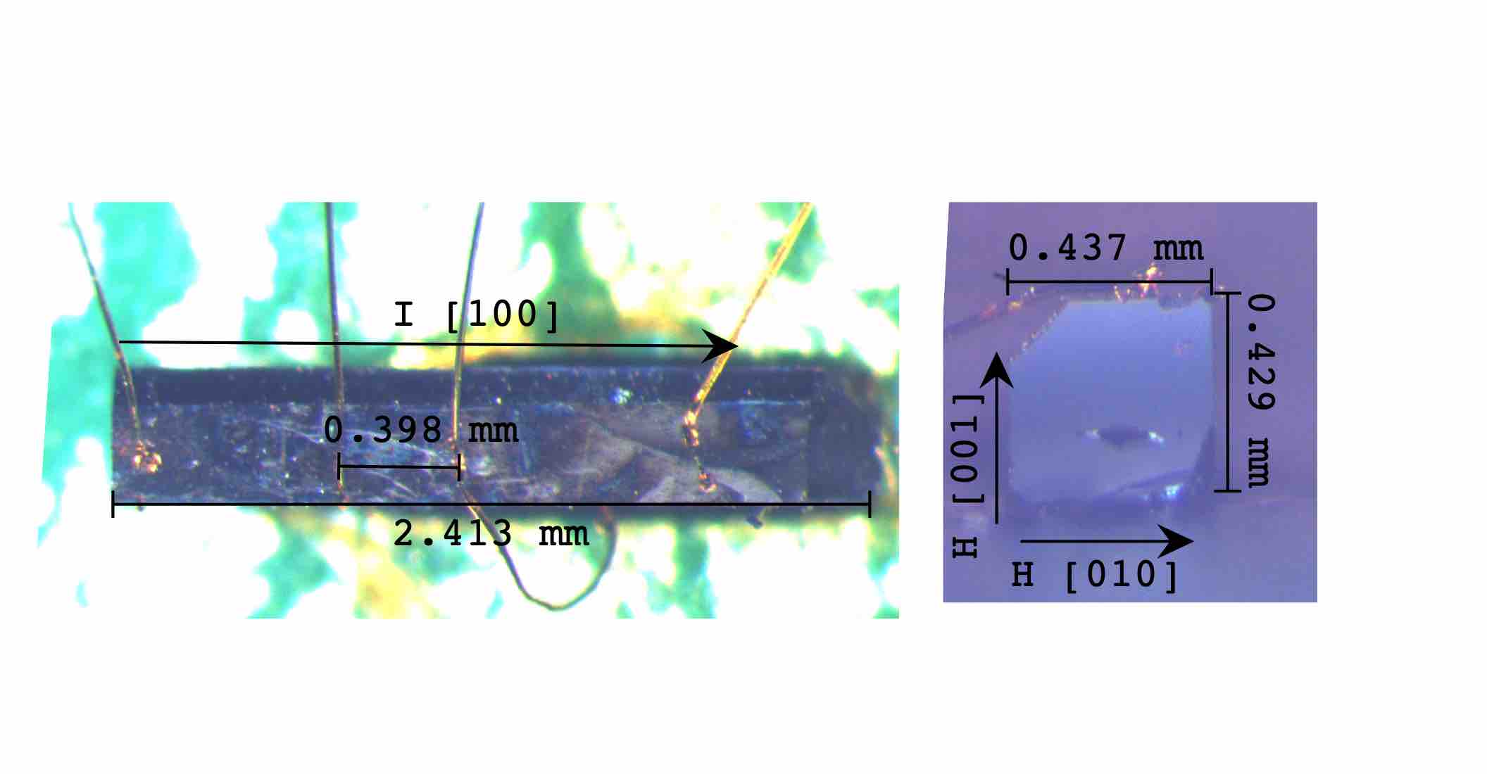
The demagnetization contribution can be calculated, if we know the magnetoresistance as a function of the magnetization (see for example Süllow et al. 2000), using the formula for the demagnetization factor Aharoni 1998, we can then calculate this contribution. The contribution from the demagnetization to the AMRO depends on both the internal magnetic field and the magnetoresistance . The demagnetizing factor for rectangular ferromagnetic prisms was given by Aharoni 1998. If for example the sample does not have a square cross-section (for example, , as shown in Fig. 1a).), then if , rotating the sample around the direction of the current flow () from the direction to the direction is equivalent to an increase in the magnetic field (). As the magnetoresistance is negative, the effect of demagnetization would be that . Thus for such a sample, the . For a given direction, the internal field in a sample is defined as Coey 2001:
| (4) | ||||
| (5) | ||||
| (6) |
Here, is the applied field and is the magnetization as a function of and . The difference in the internal magnetic field, for when the magnetic field is applied along a different geometric axis, can then be calculated using demagnetization factor Aharoni 1998. If we know the magnetization for a given applied field, we can then compute the internal field, which is the sum of the applied magnetic field plus the induced magnetization corrected by the demagnetization. We can find the induced magnetization for a given applied field with the help of Eq. 6, using a mean field approximation Rodríguez and Blanco 2005. The use of a mean field approximation for finding the magnetization is justified, since it describes the field dependence of the specific heat well, as is shown in Fig. 8.
To find the magnetization, we numerically solve the following set of equations Rodríguez and Blanco 2005:
| (7) | ||||
| (8) | ||||
| (9) | ||||
| (10) |
Here, is the Brillouin function, is the total angular momentum of of EuB6, the Curie-Weiss temperature of 12.6 K, the -factor is 2 and is the number of magnetic atoms per volume. However, in order to be able to calculate the demagnetization contribution , the magnetization dependence of the electrical resistivity has to be measured.
Madjumdar and Littlewood proposed that the magnetoresistance in metallic ferromagnets, and doped magnetic semiconductors should be negative, and proportional to the square field induced magnetization Majumdar and Littlewood 1998. In their theory, this behavior is due to the suppression of the magnetic fluctuations by the applied magnetic field. Such a behavior was reported by Süllow et al. 2000, i.e., . We carried out magnetoresistance measurements on an EuB6 sample with an almost square cross-section (sample #1 in Table 1, with , as shown in Fig. 1 of the Supplementary Materials). The results of these measurements are shown in Fig. 9 for 15 K and 20 K. For comparison we also show data extracted from Süllow et al. 2000. Our data does follow a power-law:
| (11) | ||||||||
| (12) |
and agrees with the exponent of two at low field above . Using the factor found in equation 11 and the charge carrier concentration, we can determine the position of our measurements in the plot presented by Madjumdar and Littlewood. Our factor is equal to 65, our charge carrier concentration is 5 cm-3 at low field and temperature of 20 K and our magnetic correlation length is 4.18 Å. The charge carrier concentration was taken from Hall coefficient measurements. These values take us in the same region as other EuB6 experiments Süllow et al. 2000. The first indication that is indeed due to demagnetization comes from the fact that it is commensurate with the component from the Fermi surface. As this component is linked to the shape of the cross-section, and the crystal habit is given by the cubic symmetry of EuB6, this is the expected behavior. We used Eq. 12 to calculate the two-fold AMRO component due to a combination of demagnetization effects and a large CMR in EuB6. The result of this calculation is shown in Fig. 10 as the red dashed line for a temperature of 15 K, and in an applied magnetic field of 0.5 T. Here, we calculated as function of the ratio of the demagnetization factor using a sample length of 1 mm.
Appendix B Aluminum inclusions
Previous interpretations of dHvA Fermi surface measurements of SmB6 were plagued by aluminum inclusions, see Refs. Phelan et al. 2016; Thomas et al. 2019. It was found that the aluminum inclusions are epitaxial single crystals co-oriented with the direction SmB6. We would expect the same growth direction for aluminum inclusions in EuB6. Such inclusion, if present, would then lead to four-fold AMRO pattern Balcombe 1963, with the same angle dependence as observed at high temperatures and high magnetic fields in EuB6. Thus, the lowering of the symmetry in the AMRO from four-fold to two-fold in EuB6 cannot be explained by the presence of epitaxial aluminum inclusions.
Appendix C AMRO calculations
In Eq. 3 of the manuscript we calculated a numerical integral over the Fermi Surface , which is shown in Fig. 3 of the manuscript. The total Fermi energy for one closed pocket (for example the electron band at position X) is Ciftja 2019:
| (13) | ||||
| (14) | ||||
| (15) |
where is the minor axis, and is the major axis of the elliptical pockets. These axes are linked to the volume of the Fermi volume, and hence, to the charge carrier density. So, we can obtain the minor axis from the ratio of the radii , and the density of charge carriers as:
| (16) |
Here, and will be different for the two bands (electrons and holes). The velocity of the charge carriers was calculated as follows:
| (17) |
and
| (18) |
where is a wave vector on the Fermi surface. For the propagation of the particle along a trajectory on the Fermi surface, we use the following equation of motion:
| (19) |
where is the applied magnetic field at specific angles and . The integral over time was taken from 0 to 9, giving time for the particle to do more than one revolution around the Fermi surface and for the integral to converge. In the case of EuB6 the scattering rate reported by Ref. Snow et al. 2001 cm s-1 is smaller than the cyclotron frequency ( s-1). This means that in EuB6 the electrons complete more than one revolution around the Brillouin zone before they scatter. Also, in EuB6 the Fermi pockets are far from the Brillouin zone boundaries. As a consequence, for EuB6 the contribution from an anisotropic scattering rate can be neglected. This is very different from the situation in Tl2Ba2Cu1O6+δ Analytis et al. 2007. In order to speed up calculations, we also assumed a uniform density of the charge carriers.
| Values | Electron band | Hole band |
|---|---|---|
| Aronson et al. 1999 | 1.6 | 1.8 |
| Wigger et al. 2004 | 0.24 | 0.29 |
| Snow et al. 2001 | 8.5 cm-1 | 8.5 cm-1 |
| Wigger et al. 2004 | 6.7 1019 cm-3 | 6.1 1019 cm-3 |
| Zhang et al. 2008 | 3.23 1019 cm-3 | 3.05 1019 cm-3 |
| 5 1019 cm-3 | 5 1019 cm-3 |
References
- Lilly et al. (1999) M. P. Lilly, K. B. Cooper, J. P. Eisenstein, L. N. Pfeiffer, and K. W. West, Phys. Rev. Lett. 82, 394 (1999).
- Borzi et al. (2007) R. A. Borzi, S. A. Grigera, J. Farrell, R. S. Perry, S. J. S. Lister, S. L. Lee, D. A. Tennant, Y. Maeno, and A. P. Mackenzie, Science 315, 214 (2007).
- Kivelson et al. (1998) S. A. Kivelson, E. Fradkin, and V. J. Emery, Nature 393, 550 (1998).
- MacDonald and Fisher (2000) A. H. MacDonald and M. P. A. Fisher, Phys. Rev. B 61, 5724 (2000).
- Cheong et al. (1991) S.-W. Cheong, G. Aeppli, T. E. Mason, H. Mook, S. M. Hayden, P. C. Canfield, Z. Fisk, K. N. Clausen, and J. L. Martinez, Phys. Rev. Lett. 67, 1791 (1991).
- Tranquada et al. (1997) J. M. Tranquada, J. D. Axe, N. Ichikawa, A. R. Moodenbaugh, Y. Nakamura, and S. Uchida, Phys. Rev. Lett. 78, 338 (1997).
- Ando et al. (2002) Y. Ando, K. Segawa, S. Komiya, and A. N. Lavrov, Phys. Rev. Lett. 88 (2002).
- Hinkov et al. (2008) V. Hinkov, D. Haug, B. Fauque, P. Bourges, Y. Sidis, A. Ivanov, C. Bernhard, C. T. Lin, and B. Keimer, Science 319, 597 (2008).
- Ramshaw et al. (2017) B. J. Ramshaw, N. Harrison, S. E. Sebastian, S. Ghannadzadeh, K. A. Modic, D. A. Bonn, W. N. Hardy, R. Liang, and P. A. Goddard, npj Quantum Materials 2 (2017).
- Chuang et al. (2010) T.-M. Chuang, M. P. Allan, J. Lee, Y. Xie, N. Ni, S. L. Bud’ko, G. S. Boebinger, P. C. Canfield, and J. C. Davis, Science 327, 181 (2010).
- Fernandes et al. (2014) R. M. Fernandes, A. V. Chubukov, and J. Schmalian, Nature Phys. 10, 97 (2014).
- Watson et al. (2015) M. D. Watson, T. K. Kim, A. A. Haghighirad, N. R. Davies, A. McCollam, A. Narayanan, S. F. Blake, Y. L. Chen, S. Ghannadzadeh, A. J. Schofield, M. Hoesch, C. Meingast, T. Wolf, and A. I. Coldea, Phys. Rev. B 91, 155106 (2015).
- Pomeranchuk (1959) I. I. Pomeranchuk, J. Exp. Theo. Phys. 8, 361 (1959).
- Dell’Anna and Metzner (2007) L. Dell’Anna and W. Metzner, Phys. Rev. Lett. 98, 136402 (2007).
- Yamase and Metzner (2012) H. Yamase and W. Metzner, Phys. Rev. Lett. 108, 186405 (2012).
- Ronning et al. (2017) F. Ronning, T. Helm, K. R. Shirer, M. D. Bachmann, L. Balicas, M. K. Chan, B. J. Ramshaw, R. D. McDonald, F. F. Balakirev, M. Jaime, E. D. Bauer, and P. J. W. Moll, Nature 548, 313 (2017).
- Demishev et al. (2017) S. V. Demishev, V. N. Krasnorussky, A. V. Bogach, V. V. Voronov, N. Y. Shitsevalova, V. B. Filipov, V. V. Glushkov, and N. E. Sluchanko, Sci. Rep. 7, 17430 (2017).
- Aronson et al. (1999) M. C. Aronson, J. L. Sarrao, Z. Fisk, M. Whitton, and B. L. Brandt, Phys. Rev. B 59, 4720 (1999).
- Zhang et al. (2008) X. Zhang, S. von Molnár, Z. Fisk, and P. Xiong, Phys. Rev. Lett. 100, 1 (2008).
- Massidda et al. (1996) S. Massidda, A. Continenza, T. M. de Pascale, and R. Monnier, Physik B Condensed Matter 102, 83 (1996).
- Tromp et al. (2001) H. Tromp, P. Kelly, P. van Gelderen, P. Bobbert, and G. Brocks, Phys. Rev. Lett. 87, 16401 (2001).
- Kim et al. (2013) J. Kim, W. Ku, C.-C. Lee, D. S. Ellis, B. K. Cho, A. H. Said, Y. Shvyd’ko, and Y.-J. Kim, Phys. Rev. B 87, 155104 (2013).
- Süllow et al. (1998) S. Süllow, I. Prasad, M. Aronson, J. Sarrao, Z. Fisk, D. Hristova, A. Lacerda, M. Hundley, A. Vigliante, and D. Gibbs, Phys. Rev. B 57, 5860 (1998).
- Degiorgi et al. (1997) L. Degiorgi, E. Felder, H. Ott, J. Sarrao, and Z. Fisk, Phys. Rev. Lett. 79, 5134 (1997).
- Süllow et al. (2000) S. Süllow, I. Prasad, M. Aronson, S. Bogdanovich, J. Sarrao, and Z. Fisk, Phys. Rev. B 62, 11626 (2000).
- Pohlit et al. (2018) M. Pohlit, S. Rössler, Y. Ohno, H. Ohno, S. von Molnár, Z. Fisk, J. Müller, and S. Wirth, Phys. Rev. Lett. 120 (2018).
- Nyhus et al. (1997) P. Nyhus, S. Yoon, M. Kauffman, S. L. Cooper, Z. Fisk, and J. Sarrao, Phys. Rev. B 56, 2717 (1997).
- Brooks et al. (2004) M. L. Brooks, T. Lancaster, S. J. Blundell, W. Hayes, F. L. Pratt, and Z. Fisk, Phys. Rev. B 70, 20401 (2004).
- Zhang et al. (2009) X. Zhang, L. Yu, S. von Molnár, Z. Fisk, and P. Xiong, Phys. Rev. Lett. 103, 106602 (2009).
- Das et al. (2012) P. Das, A. Amyan, J. Brandenburg, J. Müller, P. Xiong, S. von Molnár, and Z. Fisk, Phys. Rev. B 86, 184425 (2012).
- Manna et al. (2014) R. S. Manna, P. Das, M. de Souza, F. Schnelle, M. Lang, J. Müller, S. von Molnár, and Z. Fisk, Phys. Rev. Lett. 113, 067202 (2014).
- Kim et al. (2008) J. Kim, Y. J. Kim, J. Kuneš, B. K. Cho, and E. J. Choi, Phys. Rev. B 78, 1 (2008).
- Wegener and Littlewood (2002) L. Wegener and P. Littlewood, Phys. Rev. B 66, 224402 (2002).
- (34) G. Beaudin, A. Désilets-Benoit, R. Arnold, S. Samothrakitis, K. Stenning, M. Nicklas, S. Gerber, N. Egetenmeyer, J. L. Gavilano, M. Kenzelmann, R. Cubitt, C. Dewhurst, M. Laver, and A. D. Bianchi, in preparation .
- Henggeler et al. (1998) W. Henggeler, H. Ott, D. P. Young, and Z. Fisk, Solid State Commun. 108, 929 (1998).
- Wigger et al. (2004) G. A. Wigger, R. Monnier, H. R. Ott, D. P. Young, and Z. Fisk, Phys. Rev. B 69, 125118 (2004).
- Yamaji (1989) K. Yamaji, J. Phys. Soc. Jpn 58, 1520 (1989).
- Yagi et al. (1990) R. Yagi, Y. Iye, T. Osada, and S. Kagoshima, J. Phys. Soc. Jpn 59, 3069 (1990).
- Bergemann et al. (2003) C. Bergemann, A. P. Mackenzie, S. R. Julian, D. Forsythe, and E. Ohmichi, Adv. Phys. 52, 639 (2003).
- Hussey et al. (2003) N. E. Hussey, M. Abdel-Jawad, A. Carrington, A. P. Mackenzie, and L. Balicas, Nature 425 (6960), 814 (2003).
- Urbano et al. (2004) R. R. Urbano, P. G. Pagliuso, C. Rettori, S. B. Oseroff, J. L. Sarrao, P. Schlottmann, and Z. Fisk, Phys. Rev. B 70, 140401 (2004).
- Glushkov et al. (2009) V. Glushkov, M. Anisimov, A. Bogach, S. Demishev, V. Ivanov, N. Samarin, A. Dukhnenko, N. Shitsevalova, K. Flachbart, and N. Sluchanko, J. Phys.: Conf. Series 150, 022014 (2009).
- Fisk et al. (1979) Z. Fisk, D. C. Johnston, and B. Cornut, J. Appl. Phys. 50, 4 (1979).
- Goodrich et al. (1998) R. G. Goodrich, N. Harrison, J. J. Vuillemin, A. Teklu, D. W. Hall, Z. Fisk, D. Young, and J. Sarrao, Phys. Rev. B 58, 14896 (1998).
- Abdel-Jawad et al. (2006) M. Abdel-Jawad, M. P. Kennett, L. Balicas, A. Carrington, A. P. Mackenzie, R. H. McKenzie, and N. E. Hussey, Nature Physics 2, 821 (2006).
- Denlinger et al. (2002) J. Denlinger, J. Clack, J. Allen, G. H. Gweon, D. Poirier, C. Olson, J. Sarrao, A. Bianchi, and Z. Fisk, Phys. Rev. Lett. 89, 1 (2002).
- Chambers (1952) R. G. Chambers, Proceedings of the Physical Society. Section A 65, 458 (1952).
- Snow et al. (2001) C. S. Snow, S. L. Cooper, D. P. Young, Z. Fisk, A. Comment, and J.-P. Ansermet, Phys. Rev. B 64, 174412 (2001).
- Matt et al. (2015) C. E. Matt, C. G. Fatuzzo, Y. Sassa, M. Månsson, S. Fatale, V. Bitetta, X. Shi, S. Pailhès, M. H. Berntsen, T. Kurosawa, M. Oda, N. Momono, O. J. Lipscombe, S. M. Hayden, J.-Q. Yan, J.-S. Zhou, J. B. Goodenough, S. Pyon, T. Takayama, H. Takagi, L. Patthey, A. Bendounan, E. Razzoli, M. Shi, N. C. Plumb, M. Radovic, M. Grioni, J. Mesot, O. Tjernberg, and J. Chang, Phys. Rev. B 92, 134524 (2015).
- Kapitza (1929) P. Kapitza, Proc. R. Soc. A 123, 292 (1929).
- Jones and Zener (1934) H. Jones and C. Zener, Proc. R. Soc. A 145, 268 (1934).
- Gao et al. (2021) S.-Y. Gao, S. Xu, H. Li, C.-J. Yi, S.-M. Nie, Z.-C. Rao, H. Wang, Q.-X. Hu, X.-Z. Chen, W.-H. Fan, J.-R. Huang, Y.-B. Huang, N. Pryds, M. Shi, Z.-J. Wang, Y.-G. Shi, T.-L. Xia, T. Qian, and H. Ding, Phys. Rev. X 11, 021016 (2021).
- Zhitomirsky and Rice (2000) M. E. Zhitomirsky and T. M. Rice, Phys. Rev. B 62, 1492 (2000).
- Barzykin and Gor’kov (2000) V. Barzykin and L. P. Gor’kov, Physical Review Letters 84, 2207 (2000).
- Balents and Varma (2000) L. Balents and C. M. Varma, Physical Review Letters 84, 1264 (2000).
- Bałanda (2013) M. Bałanda, Acta Physica Polonica A 124, 964 (2013).
- Bianconi and Saini (2006) A. Bianconi and N. Saini, Stripes and Related Phenomena, Selected Topics in Superconductivity (Springer US, 2006).
- Booth et al. (2001) C. H. Booth, J. Sarrao, M. Hundley, A. Cornelius, G. Kwei, A. Bianchi, Z. Fisk, and J. Lawrence, Phys. Rev. B 63, 224302 (2001).
- Awschalom and Flatté (2007) D. D. Awschalom and M. E. Flatté, Nature Phys. 3, 153 (2007).
- Rodríguez and Blanco (2005) J. F. Rodríguez and J. A. Blanco, Physica Scripta 71, CC19 (2005).
- Coqblin (1977) B. Coqblin, The Electronic Structure of Rare-Earth Metals and Alloys: the Magnetic Heavy Rare-Earths, A Anouk (Academic Press, 1977).
- Ambrosini et al. (1999) B. Ambrosini, J. L. Gavilano, P. Vonlanthen, H. R. Ott, D. P. Young, and Z. Fisk, Phys. Rev. B 60, 3361 (1999).
- Aharoni (1998) A. Aharoni, J. of App. Phys. 83, 3432 (1998).
- Coey (2001) J. M. D. Coey, Magnetism and Magnetic Materials (Cambridge University Press, 2001).
- Süllow et al. (2000) S. Süllow, I. Prasad, S. Bogdanovich, M. C. Aronson, J. L. Sarrao, and Z. Fisk, J. of App. Phys. 87, 5591 (2000).
- Majumdar and Littlewood (1998) P. Majumdar and P. B. Littlewood, Nature 395, 479 (1998).
- Phelan et al. (2016) W. A. Phelan, S. M. Koohpayeh, P. Cottingham, J. A. Tutmaher, J. C. Leiner, M. D. Lumsden, C. M. Lavelle, X. P. Wang, C. Hoffmann, M. A. Siegler, N. Haldolaarachchige, D. P. Young, and T. M. McQueen, Scientific Reports 6, 20860 (2016).
- Thomas et al. (2019) S. Thomas, X. Ding, F. Ronning, V. Zapf, J. Thompson, Z. Fisk, J. Xia, and P. Rosa, Phys. Rev. Lett. 122, 166401 (2019).
- Balcombe (1963) R. J. Balcombe, Proc. R. Soc. London 275, 113 (1963).
- Ciftja (2019) O. Ciftja, Physica Scripta 94, 105806 (2019).
- Analytis et al. (2007) J. G. Analytis, M. Abdel-Jawad, L. Balicas, M. M. J. French, and N. E. Hussey, Phys. Rev. B 76 (2007).