Exact diagonalization study of the anisotropic Heisenberg model related to YbMgGaO4
Abstract
Employing exact diagonalization, we systematically study the anisotropic Heisenberg model which is related to rare-earth triangular-lattice materials. We probe its full 3D phase diagram afresh and identify a large region of quantum spin liquid (QSL) phase which can extend to the QSL region of the – triangular Heisenberg model. Furthermore, we explore the magnetization curves of different phases and reproduce the 1/3-magnetization plateau in the quantum spin liquid phase region. More importantly, to study the possible chemical disorders in real materials, we consider the randomness of exchange interactions and find no spin glass order. And there is a large region of random-singlet phase which contains strongly random spin networks, dominated by two-spin singlets, four-spin singlets and other singlet domains. Our comprehensive ED study can give detailed insightful understanding of the microscopic Hamiltonian related to the YbMgGaO4 and some other related rare-earth triangular-lattice materials.
pacs
71.27.+a, 02.70.-c, 73.43.Nq, 75.10.Jm, 75.10.Kt, 75.10.NrI Introduction
Quantum spin liquid (QSL) phase Wen 1991; *Balents2010; *XGWen2002; *Kitaev2006; *Savary2016; *Norman2016; *ZYi2017; *Broholm2020 is an exotic quantum phase of matter beyond the Landau-Ginzburg-Wilson symmetry-breaking paradigm and displays rich physics, like nonlocal fractional excitations, long-range entanglement and emergent gauge field. QSLs are more likely to be found in frustrated spin systems, such as triangular and Kagome lattices. The geometric frustration and quantum fluctuation may prevent any magnetic long-range ordering even at zero temperature.
In recent years, two-dimensional rare-earth-based frustrated magnets play an important role and gain considerable efforts to realize the QSL phase. Among that, YbMgGaO4 Li et al. 2015; Li et al. 2015a; Li et al. 2016a; Xu et al. 2016; Li et al. 2017a; Li et al. 2017b; Shen et al. 2016; Paddison et al. 2016; Li et al. 2019; Lima 2019; Majumder et al. 2020; Li 2019 and rare-earth chalcogenide family NaYbCh2(Ch = O, S, Se) Liu et al. 2018, are perfect triangular layer compounds with no structural or magnetic transition down to very low temperature. Especially, the broad continuum of magnetic excitation in the inelastic neutron scattering reveals a possible QSL with a spinon Fermi surface Shen et al. 2016; Shen et al. 2018; Dai et al. 2020. Unprecedentedly, the magnetic excitation in the fully polarized state at sufficient high field remains very broad in both energy and wave vector, indicating the possible of disorders caused by the site-mixing of Mg/Ga, giving rising to the distributions of the effective spin-1/2 factors and the magnetic couplings Li et al. 2017a. In fact, one recent experiment has observed some spin-glass-like behaviors both in the YbMgGaO4 and its sister compound YbZnGaO4 Ma et al. 2018. But other experiments seem exclude a true spin freezing in YbMgGaO4 Li et al. 2019; Ding et al. 2020.
To understand macroscopic behaviors of these materials, an easy-plane XXZ Hamiltonian with anisotropic exchange interactions was proposed to describe the effective spin-1/2 interactions Li et al. 2015a. This microscopic Hamiltonian was studied by various numerical and analytical approaches Li et al. 2016b; Liu et al. 2016; Li et al. 2017c; Li and Chen 2017; Luo et al. 2017; Zhu et al. 2017; Zhu et al. 2018; Parker and Balents 2018; Iaconis et al. 2018; Maksimov et al. 2019; Wu et al. 2019; Li 2021. In this paper, we use exact diagonalization (ED) to study this anisotropic Heisenberg model afresh. We depict the comprehensive 3D phase boundaries using extensive finite-size scaling. We have further studied the magnetic field effect and most importantly the bond randomness effect. The random-singlet phase under bond randomness in the model we studied had not been revealed before and will provide insightful understanding of the YbMgGaO4 and other related materials.
II Model and Method
The generic spin Hamiltonian of YbMgGaO4 with the next-nearest-neighbor exchange interaction on the triangular lattice reads Li et al. 2015a; Paddison et al. 2016,
where and arise from the strong spin-orbital coupling, are for the bond along three principle axes, respectively. In the following calculations, we set the XXZ anisotropic Li et al. 2018 and set as the energy unit. In the bond randomness case, the interaction strengths are uniformly distributed in the range which are controlled by . corresponds to the strongest bond randomness case. In the following, we define as the magnetic-field strengths to simplify the notations.
To get the phase boundaries, we have defined two kinds of magnetic order parameters. The first is the square sublattice magnetization for the Néel phase Watanabe et al. 2014; Shimokawa et al. 2015; Wu et al. 2019,
where represent the three sublattices of the order. The second is the square sublattice magnetization for the stripe phases Shimokawa et al. 2015; Wu et al. 2019,
where represent three kinds of stripe orders, and represent the two sublattices of -kind stripe order. We use the leading linear scaling to estimate the magnetic orders in the thermodynamic limit. The finite-size clusters used in the ED calculations are shown in Appendix A.
To eliminate other conventional orders in the quantum spin liquid region, we have also calculated three kinds of structure factors. The first one is the chiral structure factor
where and are the primitive vectors of triangular lattice and we set the lattice constant as the unit length. The second one is the dimer structure factor
where means the nearest-neighbor site of -site along direction for , respectively. means the displacement between centers of two bonds. The third one is the spin freezing order parameter
which is used to detect the possible spin-glass ordering.


III Phase diagram
The 3D phase diagram is illustrated in Fig. 1. Inside the dark yellow curve is the 120∘ Néel phase. The region in between the dark yellow curve and the green curve is a quantum spin liquid (QSL) phase. And the blue curve separates Stripe-I and Stripe-II phases. These stripe phases are Ising-like phases that have six degenerate ground states and a finite excitation gap according to the finite-size energy spectra (see Appendix C). This degeneracy will be lifted after spontaneously discrete symmetry breaking below a finite critical temperature in the thermodynamic limit Parker and Balents 2018. For the QSL, that region is a QSL based on two main reasons: one is that there are no conventional orders, including 120∘ Néel order, stripe order, dimer or valence-bond-solid order and spin-freezing order (see Fig. 3); another is that this phase can adiabatically connect to the QSL phase in the triangular Heisenberg model which can be identified by no any level crossing or avoided level crossing in the low-energy spectra and no any discontinuity or divergent tendency in the ground-state fidelity susceptibility [see Fig. 4 (b)], where the fidelity measures the amounts of shared information between two quantum states. Meanwhile, we do not see any quasidegenerate states in the QSL region from our finite-size calculations [see Fig. 4 (a)]. We conjecture that this QSL would be gapless in the thermodynamic limit similar to the triangular Heisenberg model Kaneko et al. 2014; Li et al. 2015b; Zhu and White 2015; Hu et al. 2015; Iqbal et al. 2016; Saadatmand and McCulloch 2016; Iaconis et al. 2018; Hu et al. 2019; Ferrari and Becca 2019. To give more details about this 3D phase diagram, we plot some slices in Fig. 2. The QSL boundaries are obtained by the vanishing of two kinds of magnetic orders: Néel order and stripe order. In Figs. 3(a)–3(c), we representatively show the linear extrapolations of magnetic orders along some horizontal paths on the slice. In addition, in Fig. 2, we use the contour plot to show the frustration parameter on each slice, where is the negative Curie-Weiss temperature and is the critical temperature. Here, we take the approximately as the temperature where the heat capacity gets its maximum value. Then we can confirm that the QSL region has a larger frustration parameter, especially after adding the next-nearest-neighbor interaction. The strong frustration in these regions prevents the magnetic ordering even at zero temperature. Under the guidance of the 3D phase diagram, we compare different sets of exchange parameters obtained by different research groups. Most of the parameter sets fall into the stripe phases. We only show three of them which is within or close to the QSL region, marked with A, B, and C in Fig. 2. Here we want to mention that the anisotropic exchange interactions and are weaker effects from the electron-spin resonance (ESR) measurements Li et al. 2015a. However, from our ED calculations, we find that the QSL region with only nearest-neighbor interactions needs a large , but it would be reduced by adding the next-nearest-neighbor interaction or decreasing the XXZ anisotropic , which means is important to capture spin-liquid-behavior of triangular materials if one has to neglect the possible chemical disorders and let . Compared with previous DMRG result from Ref. Zhu et al. 2018, though different is used, our QSL region in the plane is different to the DMRG one which is within the cone-like shape of 120∘ Néel ordered phase region. If we take a line path which connects two QSL regions in the and planes, we observe that the static spin structure factors always have broad peaks at around M points, not at the K points observed in Ref. Zhu et al. 2018 with an inappropriate path which is inside the 120∘ Néel phase.
IV Magnetic field effects
We have studied the magnetization curves of three magnetic ordered phases and the quantum spin liquid phase. Here in the main text, we only show the magnetization curves at of QSL region. When the magnetic field is applied perpendicular to the axis, though there is finite-size effect, we still can observe a clear “melting” 1/3-magnetization plateau [see Fig. 5 (a)]. This 1/3-plateau or “” phase is widely observed in the 120∘ Néel phase, but not in a QSL phase. The nonflatness of this plateau at zero temperature is due to the out of plane anisotropic interaction . When the further increases in the QSL region, this plateau melts to be a nonlinear rough curve. Another contribution to the nonflatness of the plateau without bond randomness is the temperature. When the temperature increases, the plateau will further melt to become a rough or even linear curve, which is shown in the inset of Fig. 5(a). For the spin structure factor , we can observe that the spectral weight shifts from M points in the zero field to the K points in the sufficient strong field around the 1/3-magnetization plateau, and then transfers to the point in the fully polarized region. Interestingly, the recent experiment on the YbMgGaO4 Bachus et al. 2020; Steinhardt et al. 2019 with very low temperature has discovered the nonlinearity of the magnetization curve which may be a signature of the remnant of 1/3-magnetization plateau. The DMRG and classical Monte Carlo simulations Steinhardt et al. 2019 using the set of parameters [see Fig. 2 (c)] have reproduced the nonlinearity of the magnetization curve. Here, our ED method has reproduced the similar behaviors not only in the set of parameters but also in the large region of QSL phase (see Appendix E). What’s more, adding do not obviously change the flatness of the plateau, but the interval of the 1/3-plateau will shrink and disappear, while the 1/2-plateau will appear at larger Nakano and Sakai 2017. In addition, we have also studied the magnetization curves with the magnetic field parallel to the axis which can be seen in Fig. 6. The 1/3-plateau seems still visible at , but has a quite narrow interval which is due to the easy-plane anisotropy and the out of plane anisotropic interactions .
V Bond randomness effects
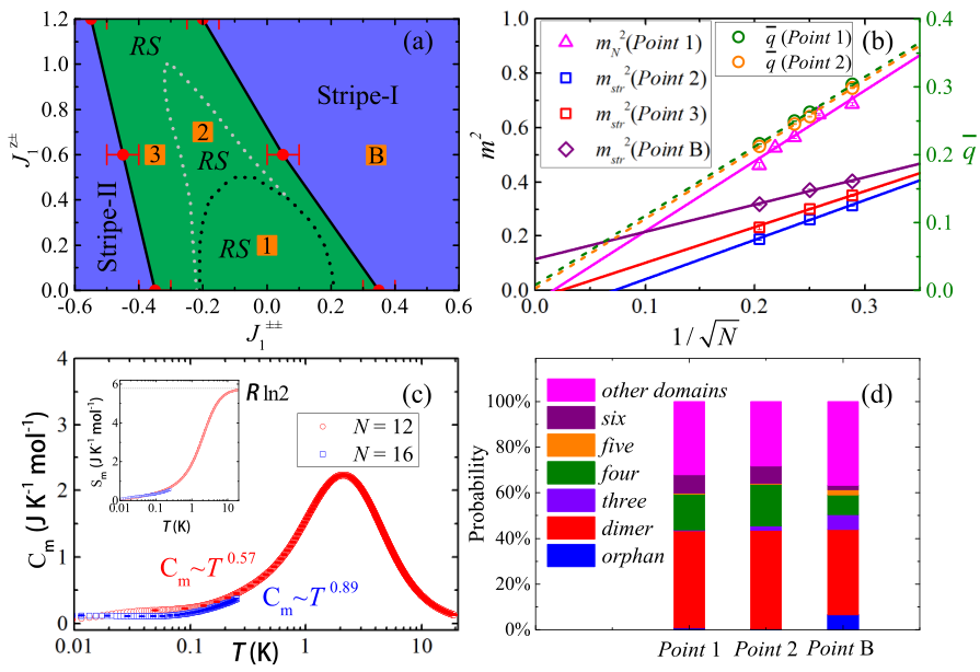
To study the possible chemical disorders in real materials, like Ga/Mg mixing in YbMgGaO4, we add uniform bond randomness into the Hamiltonian. Other distributions of the random exchange interactions do not change the conclusion qualitatively. For two stripe phases with finite excitation gaps, these magnetic orders deep into magnetic phases are stable to the bond randomness and persist up to the strongest randomness . Surprisingly, at B set of parameters, though the stripe order is still finite [see Fig. 7(b)], the magnetic heat capacity under the strongest bond randomness [see Fig. 7(c)] is similar to the experimental results Li et al. 2015; Li et al. 2015a; Xu et al. 2016; Paddison et al. 2016; Ma et al. 2018, other sets of parameters cannot reproduce the correct shape of the heat capacity. And the power-law exponents are and for 12 and 16 clusters, respectively. This power-law heat capacity is due to the nonzero density of low-lying excitations under bond randomness Kimchi et al. 2018; Kawamura and Uematsu 2019. For the Néel order, it is fragile to bond randomness, but it can persist up to a critical bond randomness strength Wu et al. 2019. So in the strongest bond randomness case, not only the QSL region and the entire phase region but also the stripe phase regions which are close to the phase boundaries [see the phase diagram in Figs. 7(a) and 7(b)] will show nonmagnetic spin-liquid-like behavior. To detect the possible spin-glass order induced by the bond randomness, we show the average spin freezing parameters in Fig. 7(b). They all are extrapolated to zero. There would be no spin-glass order even in the strongest bond randomness. This nonmagnetic spin-liquid-like phase in the limit is actually a 2D analog of random-singlet (RS) phase Ma et al. 1979; Fisher 1994; Kimchi et al. 2018; Kawamura and Uematsu 2019.

To describe this phase more clearly, we analyze the distribution of different spin domains under some different random exchange interaction configurations in Fig. 7(d). In RS phase region, we find mostly the local two-spin singlets or dimers (), four-spin singlets or resonating dimers ( for 1 and for 2) and other larger singlet domains with even number of spins (resonating dimer domains). However, it is hard to find distinct orphan spins ( for 1 and for 2) and long-distance two-spin singlets in RS phase region. In contrast, in stripe phase like the set of parameters, the fraction of orphan spins () becomes significant. Furthermore, the spin domains with odd numbers of spins also become nonnegligible. These domains with odd number of sites (including the orphan spins) will contribute to the Curie-law of magnetic susceptibility at low temperature. More significantly, larger domains with stripe order contribute to the nonzero average magnetic order under the bond randomness. However, the finite temperature would further fragment the stripe ordered domains making it hard to be detected in experiment. In order to build an intuition of the random spin networks, in Fig. 8, we representatively show the nearest-neighbor spin correlations under specific bond-randomness configurations at 2 and B, respectively. We can see the formations of orphan spins (marked by green arrows), two-spin singlets (marked by dotted oval box), four-spin singlets (resonating two types of singlet pairs marked by yellow and purple oval box) and other larger spin domains. Here we set the criterion of two spins belong to the same domain as the spin correlation between them is lower than (see Ref. Kawamura and Uematsu 2019 for more details). The singlet domains under bond randomness can help to clarify the continuous low-energy excitation and the absence of spinon contribution to thermal conductivity Ma et al. 2018; Li et al. 2019; Li et al. 2017b. And the last not the least, for the magnetization curve, the 1/3-magnetization plateau will further melt by the randomness of exchange interactions and -factors Watanabe et al. 2014, similar to the temperature effect. There would be no distinct 1/3-magnetization plateau under the strongest bond randomness Bachus et al. 2020.
VI Summary and discussion
In summary, we have used extensive finite-size scalings with ED to get the entire phase diagram in the 3D parameter space. Besides two gapped stripe phases and 120∘ Néel phase, there is a large QSL region extending to the QSL phase of the triangular Heisenberg model. After applying external magnetic fields, a 1/3-magnetization plateau can be observed at large region of QSL phase when the magnetic field is perpendicular to the axis. Most importantly, in the strongest bond randomness case, numerical result shows a large region of spin-liquid-like phase which is a 2D analog of random-singlet phase. It contains two-spin singlets, four-spin singlets and other larger spin singlets which have not been unveiled in the model we studied. In addition, our 3D phase diagram with different XXZ anisotropy (see Appendix G) can also help to understand the QSL like behavior in AYbCh2 (A=Na and Cs, Ch=O,S,Se) Liu et al. 2018; Dai et al. 2020; Baenitz et al. 2018; Ranjith et al. 2019a; Ding et al. 2019; Xing et al. 2019; Sarkar et al. 2019; Guo et al. 2020; Ma et al. 2020; Bordelon et al. 2020a; Bordelon et al. 2020b; Ranjith et al. 2019b; Jia et al. 2020; Zhang et al. 2020a; Zhang et al. 2020b; Zhang et al. 2021; Sichelschmidt et al. 2019; Sichelschmidt et al. 2020; Zangeneh et al. 2019, Na2BaCo(PO4)2 Zhong et al. 2019; Li et al. 2020; Lee et al. 2021.
Both YbMgGaO4 and NaYbCh2 share the same space symmetry group and the perfect triangular magnetic layers which consist of Yb3+ ions. Recent experiments Liu et al. 2018; Baenitz et al. 2018; Ding et al. 2019; Guo et al. 2020; Bordelon et al. 2020a; Bordelon et al. 2020b have revealed that the interlayer Yb-Yb distance in NaYbO2 and NaYbS2 is shorter than YbMgGaO4, which means the interlayer interactions may be relevant in the low temperature exchange model. A more complicated exchange Hamiltonian with the same in-plane part as the YbMgGaO4 and compass-like interlayer exchange interactions has been proposed to understand macroscopic behaviors of these materials [see Ref. Bordelon et al. 2020b for more details]. In addition, we still need to caution about the possible randomness effects on NaYbCh2, such as Na sites occupied by the Yb ions in NaYbSe2 Dai et al. 2020. All of these issues, including the interlayer interactions and magnetic impurities between Yb layers, need further study.
Acknowledgements.
Acknowledgments H.Q.W. thanks Shou-Shu Gong, Wei Zhu, and Rong-Qiang He for helpful discussions. D.X.Y. is supported by NKRDPC-2018YFA0306001, NKRDPC-2017YFA0206203, NSFC-11974432, GBABRF-2019A1515011337, and Leading Talent Program of Guangdong Special Projects. H.Q.W. is supported by NSFC-11804401 and the Fundamental Research Funds for the Central Universities (Grant No. 19lgpy266).Appendix A Finite-size clusters
In this paper, we mainly use Lanczos exact diagonalization to get the 3D phase diagram and the low-energy spectrum. Meanwhile, we also employ full exact diagonalization to study the finite-temperature properties, such as heat capacity and magnetic susceptibility. To reduce the computational cost, we have used translation symmetry to do block diagonalization. The largest system size in the Lanczos calculations is 32 with the subspace of the largest block up to 0.13 billion.
Ten clusters are mainly used in our ED calculations which are shown in Fig. 9, denoted as , , , , , , , , and , respectively. The , , , , and clusters have three momentum points which are significant for the stripe phases. These three-momentum points denote as , where are primitive lattice vectors in reciprocal space, is the lattice constant. Among these five clusters with even number of lattice site, the 12 and 24b clusters also contain two K points, . The K points are important for 120∘ Néel phase and the 1/3-magnetization plateau phase or “” phase. So we use the , , , , , and clusters which contain K points to do the linear extrapolations of 120∘ Néel order and to study the 1/3-magnetization plateau. In the extrapolation of the spin freezing order parameters, we also use cluster.
Here, we want to mention that three momentum points are nonequivalent in the , and clusters which do not respect the rotation symmetry. Therefore, there may be only one point which has a broad peak in the spin structure factor of QSL region [see Fig. 5(c), Fig. 6(c) in the main text, and Fig. 29(b1)–29(b4)]. We should see the diffuse magnetic scattering at around all three points when we use the clusters which have equivalent points, such as [see Fig. 29(a1)–29(a4)] and clusters.
Appendix B Conventional orders
We have representatively shown the linear extrapolations of 120∘ Néel order and the stripe orders in the main text. Here, we want to show more details about the extrapolations, which can be seen in Figs. 10 and 11. The magnetic order parameters (square root of the extrapolated results) obtained from Figs. 10(a1) and 10(a2), 10(b1) and 10(b2) are shown in Figs. 10(a3) and 10(b3), respectively. Here, we mention that the stripe phases are Ising-like phases which have strong magnetic orders and weaker quantum fluctuations. Therefore, the linear extrapolations of magnetic orders are good enough to identify the phase boundaries. The extrapolated results will not change much when using some larger system sizes.
To eliminate other conventional orders in the nonmagnetic phase region, we have also calculated the chiral and dimer structure factors. In our finite-size calculations, we find the peak positions of and vary between different clusters, which can be seen in Fig. 12. So we use to represent the wave vector where the peak is in Fig. 3(d) of the main text. We get the vanishing order parameters of these two conventional ordering using linear extrapolations. Therefore, the large region of nonmagnetic phase in the 3D parameter space (see Figs. 1 and 2) has no 120∘ Néel order, stripe orders, chiral order, dimer order and spin-freezing order [see Fig. 3(d)], and it is a quantum spin liquid phase.
Appendix C Stripe-I and Stripe-II phases

We have calculated the low-energy spectra of different phases and find that there are six degenerate ground states in Stripe-I and Stripe-II phases, as shown in Fig. 13. These six degenerate ground states are in the translation invariant momentum sectors . Three of them are in the sector, while the other three distribute into three sectors. We can use finite-size scaling of energy gaps to verify the degeneracy in the thermodynamic limit which is shown in Fig. 14.
Previous classical Monte Carlo study from Ref. Parker and Balents 2018 has shown that there are six basic spin-orbital-lock stripe configurations which differentiate by three choices of the principal lattice directions that stripes run along and two spin orientations within each stripe. For , in the stripe-I phase, the spins lay in the plane and point perpendicular to the stripes (see Fig. 1), while in the stripe-II phase, the spins also lay in the plane but point along the principal axes (see Fig. 1). The nonzero will tilt the spins out of plane by an angle with the axis.
Appendix D Frustration parameter
The frustration parameter is defined as , where is the negative Curie-Weiss temperature and is the critical temperature. We take the approximately as the temperature where the magnetic heat capacity gets its maximum value. Actually, works well in the stripe-I and stripe-II phases. However, in quantum spin liquid phase region, is zero. In fact, the frustration parameter should be diverge. And the heat capacity still has a broad maximum at finite . In the 120∘ Néel phase, the and interactions break the continuous symmetry of the XXZ model. Especially, the interaction would tilt the spins out of plane. Then whether the 120∘ Néel phase has a gap and a finite critical temperature are still unclear, which need further study in the future. In any case, we can expect that should be less than the . Therefore, the frustration parameter in the 120∘ Néel phase is underestimate. Even though, using may not correctly estimate the actual frustration parameter. We still can use this approximation to compare the frustration of different phase regions in the 3D parameter space. As we have shown in the Fig. 2 of the main text, the nonmagnetic quantum spin liquid region has a larger frustration parameter compared to other magnetic ordered phase regions, that is consistent with phase boundaries obtained by extrapolations of magnetic orders.
Appendix E Magnetization curves
In this sector, we want to show more magnetization curves at different phases, including 120∘ Néel phase, Stripe-I phase, and quantum spin liquid phase. The magnetization curves with some sets of parameters in the quantum spin liquid region are representatively shown in Fig. 16. In Figs. 16(a1) and 16(a2), since the out-of-plane interaction is large, it seems that the 1/3-magnetization plateau is already melted to be invisible, especially for the curve obtained by cluster. And a more linear curve (in the thermodynamic limit) is observed when applying the field parallel to the axis. While for Figs. 16(b1) and 16(c1), the interaction is small or zero, so we can reproduce flat 1/3-magnetization plateaux.
We have also calculated the magnetization curves of 120∘ Néel phase and Stripe-I phase in Fig. 17. In the 120∘ Néel phase, the 1/3-magnetization plateau is clearly seen. The nonflatness depends on the interaction. In the Stripe-I phase, there is no 1/3-magnetization plateau induced by two kinds of magnetic fields.
To show the effects of different exchange interactions, like , on the 1/3-magnetization plateau, we use cluster to show the change of magnetic curves with these parameters, which are shown in Fig. 18. When are small and the system is in 120∘ Néel phase, the 1/3-magnetization plateau is flat. In the quantum spin liquid phase region with large , the 1/3-magnetization plateau is melted to nonlinear rough curve, see Fig. 18(a1). When we increase and keep , the flatness of plateau is nearly unchanged. After which drives system into Stripe-I phase, the plateau quickly melts to a linear curve, see Fig. 18(b1). For the XXZ model, in the 120∘ Néel and the QSL phase regions, the 1/3-magnetization plateau is flat and has nonzero width in the thermodynamic limit [see the inset of Fig. 18(c1)]. When , the system is in the stripe phase with threefold ground-state degeneracy, the 1/3-magnetization plateau disappears [see the inset of Fig. 18(c1)]. Instead, a 1/2-magnetization plateau appears.
To verify the 1/3-magnetization plateau phase is a phase. We have calculated the energy spectrum and the spin correlation functions at , see Fig. 19. From the low-energy spectrum, we find threefold quasidegenerate ground states. Through finite-size scalings, we can observe the exact degeneracy (before spontaneously symmetry breaking) and a finite-energy gap above the ground-state manifold. And we show the real-space spin correlation functions of these three ground states in Fig. 20, the structure can be clearly seen.
Appendix F VII: Bond randomness effects
To simulate chemical disorders in YbMgGaO4, we have introduced bond randomness into the Hamiltonian. And there are four sets of parameters have been frequently used to do the calculations, ; ; ; and . These four sets of parameters have been marked in Fig. 7(a) of the main text. For the Néel phase, the strongest randomness at can eliminate this magnetic order, which can be seen in Fig. 7(b) of the main text. For most of the stripe-phase region, the stripe orders are stable against the bond randomness and cannot be eliminated even in the strongest bond-randomness case, as can be seen in Fig. 7(b) of the main text. And for QSL phases, both in the clean case and the strongest bond randomness limit, the vanishing of the average spin freezing order parameter [shown in Fig. 3(d) and Fig. 7(b) of the main text] indicates the absence of spin-glass order. To confirm the convergence, we show different order parameters changing with the number of random samples in Fig. 21(d). We are confident that using at least 20 bond-randomness samples is able to get reliable randomly averaged order parameters.

Using linear extrapolations of the stripe order parameter shown in Figs. 21(a)–21(c), we obtain the phase diagram under the strongest bond randomness = 1.0, which is shown in Fig. 7(a) of the main text. In the nonmagnetic spin-liquid-like (SLL) phase region, we also show the average spin freezing order parameter to rule out the spin glass phase. This SLL phase is actually a 2D analog of random-singlet (RS) phase. To see more clear about this phase, we plot the real-space spin correlations under some representative bond randomness configurations, which are shown in Fig. 8 of the main text and Fig. 22.
In the RS phase, we can find some random distributions of nearest-neighbor two-spin singlets, four-spin singlets and other larger singlet domains. If two nearest-neighbor spins form an exact singlet, then the spin correlation between these two spins is equal to . However, due to the geometry frustration and competition between nearest-neighbor bonds sharing one of the same lattice site, two nearest-neighbor spins can approximately form a local singlet if their correlation is close to . In Fig. 8 of the main text and Fig. 22, we representatively show the two-spin singlets (or dimers) which are marked by the dotted oval boxes. For four nearest-neighbor spins forming a (plaquette) singlet, the spin correlations between diagonal sites [red solid and red dashed lines in Fig. 23(a)] are equal to which represents ferromagnetic correlation, that will contribute to the nonzero fraction of ferromagnetic correlations in the histogram of Figs. 23(a) and 23(b). Similarly, we have also found six-spin singlets which are representatively shown in Fig. 8(a2) of the main text and Fig. 22(d). Other larger singlet domains can also be found. But how do we define a spin domain? For two spins with their correlation larger than , they are disentangled in the limit Kawamura and Uematsu 2019. Therefore, we can set the criterion of two spins belonging to the same domain as the spin correlation between them is less than (see more details in Ref. Kawamura and Uematsu 2019). In Fig. 7(d) of the main text, we show the histogram of different spin domains in the RS phase. The dominant contributions are the two-spin singlets and other larger singlet domains with even number of spins. In Figs. 23(a) and 23(b), we show the distribution of nearest-neighbor spin correlations to see more details from another aspect. As we known, if two nearest-neighbor spins form a nearly singlet, then the spin correlations of other ten nearest-neighbor bonds sharing one of these two spins in the triangular lattice will be very weak. Therefore, unlike the 1D bipartite Heisenberg chain, due to the large coordination number and the geometry frustration of triangular lattice, the percentage of singlet bonds in all nearest-neighbor bonds will be small, as can be seen in Fig. 23(a). In the formation of four-spin singlet, the spin correlations of diagonal nearest-neighbor and next-nearest-neighbor bonds (for triangular lattice) are which contributes to the nonzero fraction of ferromagnetic correlations in Figs. 23(a) and 23(b).
In the Stripe-I phase, take B set of parameters () as example, we show the histogram of nearest-neighbor and next-nearest-neighbor spin correlations in Figs. 23(c) and 23(d), respectively. The bond randomness cannot fully destroy the stripe order. Therefore, we can see a large fraction of antiferromagnetic correlation ( 0.25) and ferromagnetic correlation ( 0.25) in the nearest-neighbor and the next-nearest-neighbor spin correlations.
To show how the bond randomness strength affects the ground state, we show the distribution of spin domains as a function of in Fig. 24. At B which is shown in Fig. 24(b), in the weak bond randomness regime with 0.5, because of the large excitation gap, nearly all the spins are in one domain with stripe ordering. With the increasing of the randomness, say 0.5, large domains are gradually broken into some smaller domains, especially like the two-spin singlets or dimers. While at 2 without any magnetic ordering in the clean case, spins can easily form some small singlet domains even under weak bond randomness ( = 0.2) [shown in Fig. 24(a)]. Interestingly, spins prefer to form four-spin singlets or resonating dimers when instead of two-spin singlets or dimers which dominate the case of stronger randomness ( 0.5). For the orphan or isolated spin, its fraction is nonnegligible when (4.8% at = 0.2 and 3.0% at = 0.4) and then drops to below 1% when 0.5.


The above discussions focus on ground-state properties at zero temperature. Here, we want to discuss the bond randomness effects at finite temperature. Figure 25(a) shows the magnetic heat capacity of B set of parameters which have also been shown in Fig. 7(c) of the main text. And we have used sufficient random samples to make the power-law exponent converged, which can be seen in the inset of Fig. 25 (a).
In the strong randomness case, the finite-size effect is actually not severe. So the cluster is able to capture the main physics in the strongest bond-randomness limit. In this limit, the heat capacity has a broad peak, and this peak will not diverge with the increasing system size. That means even though the ground state of the system has residual stripe order, but it may be hard to probe this order at finite temperature. Actually, previous classical Monte Carlo simulation from Ref. Parker and Balents 2018 has shown the similar behavior in the heat capacity. In the clean case, there is a single critical temperature with slowly diverging heat capacity. In the randomness case, this transition is removed by fragmenting the system into spin domains.
We have also calculated the heat capacity with other sets of parameters (especially for the sets of parameters fitting by different research groups or within the QSL phase region) under the strongest bond randomness. However, none of those can reproduce nearly the same heat capacity as the experimental one, which are show in Figs. 25 and 26. In the clean limit, whether we can get the same heat capacity as the experimental one using some sets of parameters is still an open question. Recently, a finite-temperature Lanczos methods with improved accuracy has successfully applied to Kitaev-Heisenberg model on Kagome and triangular lattices Morita and Tohyama 2020, which would be a great help to study the finite-temperature properties of the model related to YbMgGaO4 in future.
Appendix G XXZ anisotropic effects
To see how the XXZ (or easy-plane) anisotropic affects the phase diagram, we use fidelity susceptibility of cluster to get the 120∘ Néel phase boundaries under different , and use the linear extrapolations of the stripe order (mainly using and clusters) to get the phase boundaries of stripe phases. Then we obtain some phase diagrams under different which are shown in Fig. 27. When decreases, the (deformed) 120∘ Néel phase and the QSL phase regions shrink. Especially for the QSL phase, at , this phase region is too small to identify. Therefore, is a approximate critical value where the QSL disappears. In the limit of , the 120∘ Néel phase region will quickly vanish [see Fig. 28 (b)]. When is large, both of the 120∘ Néel phase and the QSL phase seem to extend to larger areas. Please remind that we have taken (actually ) as the energy unit. If we take as the new energy unit, then the area of QSL phase region may decrease to a finite constant when we increase from 1 to larger values. In the limit or , unlike the limit, the quantum spin liquid phase will survive Suzuki et al. 2019. Compared with previous DMRG study from Ref. Zhu et al. 2017 and Ref. Zhu et al. 2018, our QSL regions are more naturally located between three magnetic ordered phases due to the order-by-disorder effect and extend to the axis in the plane.
Appendix H Static and dynamical spin structure factor
The inelastic neutron scattering experiment of YbMgGaO4 has revealed a broad low-energy excitation maxima at the M point and the concentrated spectral weight at the boundary of Brillouin zone. Here we show the contour plots of the static spin structure factors of the QSL region in Fig. 29. We take a straight-line path in the 3D parameter space to show the static spin structure factors of QSL phase. The broad peaks at the M points signature short-range stripelike spin correlations in the QSL phase.
We also calculate the dynamical spin structure which can be studied by inelastic neutron scattering (INS) or x-ray Raman scattering in experiment. The dynamical spin structure factor in the QSL region can be computed by continued fraction expansion,
where label the spin indices, , and are the diagonal and subdiagonal elements of the tridiagonal Hamiltonian matrix obtained by the Lanczos method with initial vector . Here, we show the ED results using cluster in Fig. 30. At , though there are finite-size effects, we still can observe that the low-energy maxima are located at M points. And the maxima at K points are at higher energy. It seems that our ED calculations are consistent with the inelastic neutron scattering measurements of YbMgGaO4 Shen et al. 2016; Paddison et al. 2016. While using the C set of parameters, the maxima in K and M points are nearly at the same energy. It can be easy to understand this phenomenon. Starting from 120∘ Néel phase to the QSL phase, and then to a stripe phase, the spectral weight would transfer from K points to the M points.
Appendix I Exchange parameters
In Table 1, we list three sets of exchange parameters fitted by experimental data and got from Ref. Paddison et al. 2016, Ref. Li et al. 2018 and Ref. Steinhardt et al. 2019, respectively. set of parameters was used to calculate the specific heat in Fig. 25(b). set of parameters was used to calculate the magnetization curves in Figs. 16(b1) and 16(b2). set of parameters was used to calculate the specific heat in Fig. 25(a) and Fig. 7(c) of the main text. In Appendix, we also use it to show the frustration parameter in Fig. 15 of Appendix D, the magnetization curves in Figs. 17(b1) and 17(b2), the square sublattice magnetization for Stripe-I phase in Fig. 21(d), the histograms of spin correlations in Figs. 23(c) and 23(d), the distribution of spin domains with different number of spins changing with in Fig. 24(b) and the nearest-neighbor spin correlations for different random configurations in Figs. 8(b1)–8(b4) of the main text.
| 0.126 | 0.164 | 0.164 | |
|---|---|---|---|
| 1 | 1 | 1 | |
| 1.73 | 1.317 | 1.317 | |
| 0.103 | 0.341 | 0 | |
| 0 | 0.598 | 0.13 | |
| 0.22 | 0 | 0.1 | |
| 0.22 | 0 | 0.1 | |
| 0.381 | 0 | 0.132 |
References
- Wen (1991) X. G. Wen, Phys. Rev. B 44, 2664 (1991).
- Balents (2010) L. Balents, Nature 464, 199 (2010).
- Wen (2002) X.-G. Wen, Phys. Rev. B 65, 165113 (2002).
- Kitaev (2006) A. Kitaev, Annals of Physics 321, 2 (2006).
- Savary and Balents (2016) L. Savary and L. Balents, Rep. Prog. Phys. 80, 016502 (2016).
- Norman (2016) M. R. Norman, Rev. Mod. Phys. 88, 041002 (2016).
- Zhou et al. (2017) Y. Zhou, K. Kanoda, and T.-K. Ng, Rev. Mod. Phys. 89, 025003 (2017).
- Broholm et al. (2020) C. Broholm, R. J. Cava, S. A. Kivelson, D. G. Nocera, M. R. Norman, and T. Senthil, Science 367 (2020), 10.1126/science.aay0668.
- Li et al. (2015) Y. Li, H. Liao, Z. Zhang, S. Li, F. Jin, L. Ling, L. Zhang, Y. Zou, L. Pi, Z. Yang, J. Wang, Z. Wu, and Q. Zhang, Scientific Reports 5, 16419 (2015).
- Li et al. (2015a) Y. Li, G. Chen, W. Tong, L. Pi, J. Liu, Z. Yang, X. Wang, and Q. Zhang, Phys. Rev. Lett. 115, 167203 (2015a).
- Li et al. (2016a) Y. Li, D. Adroja, P. K. Biswas, P. J. Baker, Q. Zhang, J. Liu, A. A. Tsirlin, P. Gegenwart, and Q. Zhang, Phys. Rev. Lett. 117, 097201 (2016a).
- Xu et al. (2016) Y. Xu, J. Zhang, Y. S. Li, Y. J. Yu, X. C. Hong, Q. M. Zhang, and S. Y. Li, Phys. Rev. Lett. 117, 267202 (2016).
- Li et al. (2017a) Y. Li, D. Adroja, R. I. Bewley, D. Voneshen, A. A. Tsirlin, P. Gegenwart, and Q. Zhang, Phys. Rev. Lett. 118, 107202 (2017a).
- Li et al. (2017b) Y. Li, D. Adroja, D. Voneshen, R. I. Bewley, Q. Zhang, A. A. Tsirlin, and P. Gegenwart, Nature Communications 8, 15814 (2017b).
- Shen et al. (2016) Y. Shen, Y.-D. Li, H. Wo, Y. Li, S. Shen, B. Pan, Q. Wang, H. C. Walker, P. Steffens, M. Boehm, Y. Hao, D. L. Quintero-Castro, L. W. Harriger, M. D. Frontzek, L. Hao, S. Meng, Q. Zhang, G. Chen, and J. Zhao, Nature 540, 559 (2016).
- Paddison et al. (2016) J. A. M. Paddison, M. Daum, Z. Dun, G. Ehlers, Y. Liu, M. B. Stone, H. Zhou, and M. Mourigal, Nat. Phys. 13, 117 (2016).
- Li et al. (2019) Y. Li, S. Bachus, B. Liu, I. Radelytskyi, A. Bertin, A. Schneidewind, Y. Tokiwa, A. A. Tsirlin, and P. Gegenwart, Phys. Rev. Lett. 122, 137201 (2019).
- Lima (2019) M. P. Lima, Journal of Physics: Condensed Matter 32, 025505 (2019).
- Majumder et al. (2020) M. Majumder, G. Simutis, I. E. Collings, J.-C. Orain, T. Dey, Y. Li, P. Gegenwart, and A. A. Tsirlin, Phys. Rev. Research 2, 023191 (2020).
- Li (2019) Y. Li, Advanced Quantum Technologies 2, 1900089 (2019).
- Liu et al. (2018) W. Liu, Z. Zhang, J. Ji, Y. Liu, J. Li, X. Wang, H. Lei, G. Chen, and Q. Zhang, Chin. Phys. Lett. 35, 117501 (2018).
- Shen et al. (2018) Y. Shen, Y.-D. Li, H. C. Walker, P. Steffens, M. Boehm, X. Zhang, S. Shen, H. Wo, G. Chen, and J. Zhao, Nat. Comm. 9, 4138 (2018).
- Dai et al. (2020) P.-L. Dai, G. Zhang, Y. Xie, C. Duan, Y. Gao, Z. Zhu, E. Feng, C.-L. Huang, H. Cao, A. Podlesnvak, G. E. Granroth, D. Voneshen, S. Wang, G. Tan, E. Morosan, X. Wang, L. Shu, G. Chen, Y. Guo, X. Lu, and P. Dai, arXiv 2004, 06867 (2020).
- Ma et al. (2018) Z. Ma, J. Wang, Z.-Y. Dong, J. Zhang, S. Li, S.-H. Zheng, Y. Yu, W. Wang, L. Che, K. Ran, S. Bao, Z. Cai, P. Čermák, A. Schneidewind, S. Yano, J. S. Gardner, X. Lu, S.-L. Yu, J.-M. Liu, S. Li, J.-X. Li, and J. Wen, Phys. Rev. Lett. 120, 087201 (2018).
- Ding et al. (2020) Z. Ding, Z. Zhu, J. Zhang, C. Tan, Y. Yang, D. E. MacLaughlin, and L. Shu, Phys. Rev. B 102, 014428 (2020).
- Li et al. (2016b) Y.-D. Li, X. Wang, and G. Chen, Phys. Rev. B 94, 035107 (2016b).
- Liu et al. (2016) C. Liu, R. Yu, and X. Wang, Phys. Rev. B 94, 174424 (2016).
- Li et al. (2017c) Y.-D. Li, Y.-M. Lu, and G. Chen, Phys. Rev. B 96, 054445 (2017c).
- Li and Chen (2017) Y.-D. Li and G. Chen, Phys. Rev. B 96, 075105 (2017).
- Luo et al. (2017) Q. Luo, S. Hu, B. Xi, J. Zhao, and X. Wang, Phys. Rev. B 95, 165110 (2017).
- Zhu et al. (2017) Z. Zhu, P. A. Maksimov, S. R. White, and A. L. Chernyshev, Phys. Rev. Lett. 119, 157201 (2017).
- Zhu et al. (2018) Z. Zhu, P. A. Maksimov, S. R. White, and A. L. Chernyshev, Phys. Rev. Lett. 120, 207203 (2018).
- Parker and Balents (2018) E. Parker and L. Balents, Phys. Rev. B 97, 184413 (2018).
- Iaconis et al. (2018) J. Iaconis, C. Liu, G. B. Halász, and L. Balents, SciPost Phys. 4, 003 (2018).
- Maksimov et al. (2019) P. A. Maksimov, Z. Zhu, S. R. White, and A. L. Chernyshev, Phys. Rev. X 9, 021017 (2019).
- Wu et al. (2019) H.-Q. Wu, S.-S. Gong, and D. N. Sheng, Phys. Rev. B 99, 085141 (2019).
- Li (2021) S. Li, Phys. Rev. B 103, 104421 (2021).
- Li et al. (2018) Y.-D. Li, Y. Shen, Y. Li, J. Zhao, and G. Chen, Phys. Rev. B 97, 125105 (2018).
- Watanabe et al. (2014) K. Watanabe, H. Kawamura, H. Nakano, and T. Sakai, Journal of the Physical Society of Japan 83, 034714 (2014).
- Shimokawa et al. (2015) T. Shimokawa, K. Watanabe, and H. Kawamura, Phys. Rev. B 92, 134407 (2015).
- Steinhardt et al. (2019) W. M. Steinhardt, Z. Shi, A. Samarakoon, S. Dissanayake, D. Graf, Y. Liu, W. Zhu, C. Marjerrison, C. D. Batista, and S. Haravifard, arXiv 1902, 07825 (2019).
- Zhang et al. (2018) X. Zhang, F. Mahmood, M. Daum, Z. Dun, J. A. M. Paddison, N. J. Laurita, T. Hong, H. Zhou, N. P. Armitage, and M. Mourigal, Phys. Rev. X 8, 031001 (2018).
- Kaneko et al. (2014) R. Kaneko, S. Morita, and M. Imada, Journal of the Physical Society of Japan 83, 093707 (2014).
- Li et al. (2015b) P. H. Y. Li, R. F. Bishop, and C. E. Campbell, Phys. Rev. B 91, 014426 (2015b).
- Zhu and White (2015) Z. Zhu and S. R. White, Phys. Rev. B 92, 041105(R) (2015).
- Hu et al. (2015) W.-J. Hu, S.-S. Gong, W. Zhu, and D. N. Sheng, Phys. Rev. B 92, 140403(R) (2015).
- Iqbal et al. (2016) Y. Iqbal, W.-J. Hu, R. Thomale, D. Poilblanc, and F. Becca, Phys. Rev. B 93, 144411 (2016).
- Saadatmand and McCulloch (2016) S. N. Saadatmand and I. P. McCulloch, Phys. Rev. B 94, 121111(R) (2016).
- Hu et al. (2019) S. Hu, W. Zhu, S. Eggert, and Y.-C. He, Phys. Rev. Lett. 123, 207203 (2019).
- Ferrari and Becca (2019) F. Ferrari and F. Becca, Phys. Rev. X 9, 031026 (2019).
- Bachus et al. (2020) S. Bachus, I. A. Iakovlev, Y. Li, A. Wörl, Y. Tokiwa, L. Ling, Q. Zhang, V. V. Mazurenko, P. Gegenwart, and A. A. Tsirlin, Phys. Rev. B 102, 104433 (2020).
- Nakano and Sakai (2017) H. Nakano and T. Sakai, Journal of the Physical Society of Japan 86, 114705 (2017).
- Kimchi et al. (2018) I. Kimchi, A. Nahum, and T. Senthil, Phys. Rev. X 8, 031028 (2018).
- Kawamura and Uematsu (2019) H. Kawamura and K. Uematsu, Journal of Physics: Condensed Matter 31, 504003 (2019).
- Ma et al. (1979) S.-k. Ma, C. Dasgupta, and C.-k. Hu, Phys. Rev. Lett. 43, 1434 (1979).
- Fisher (1994) D. S. Fisher, Phys. Rev. B 50, 3799 (1994).
- Baenitz et al. (2018) M. Baenitz, P. Schlender, J. Sichelschmidt, Y. A. Onykiienko, Z. Zangeneh, K. M. Ranjith, R. Sarkar, L. Hozoi, H. C. Walker, J.-C. Orain, H. Yasuoka, J. van den Brink, H. H. Klauss, D. S. Inosov, and T. Doert, Phys. Rev. B 98, 220409(R) (2018).
- Ranjith et al. (2019a) K. M. Ranjith, D. Dmytriieva, S. Khim, J. Sichelschmidt, S. Luther, D. Ehlers, H. Yasuoka, J. Wosnitza, A. A. Tsirlin, H. Kühne, and M. Baenitz, Phys. Rev. B 99, 180401(R) (2019a).
- Ding et al. (2019) L. Ding, P. Manuel, S. Bachus, F. Grußler, P. Gegenwart, J. Singleton, R. D. Johnson, H. C. Walker, D. T. Adroja, A. D. Hillier, and A. A. Tsirlin, Phys. Rev. B 100, 144432 (2019).
- Xing et al. (2019) J. Xing, L. D. Sanjeewa, J. Kim, G. R. Stewart, A. Podlesnyak, and A. S. Sefat, Phys. Rev. B 100, 220407(R) (2019).
- Sarkar et al. (2019) R. Sarkar, P. Schlender, V. Grinenko, E. Haeussler, P. J. Baker, T. Doert, and H.-H. Klauss, Phys. Rev. B 100, 241116(R) (2019).
- Guo et al. (2020) J. Guo, X. Zhao, S. Ohira-Kawamura, L. Ling, J. Wang, L. He, K. Nakajima, B. Li, and Z. Zhang, Phys. Rev. Materials 4, 064410 (2020).
- Ma et al. (2020) J. Ma, J. Li, Y. H. Gao, C. Liu, y Qingyong Ren, Z. Zhang, Z. Wang, R. Chen, J. Embs, E. Feng, F. Zhu, Q. Huang, Z. Xiang, L. Chen, E. S. Choi, Z. Qu, L. Li, J. Wang, H. Zhou, Y. Su, X. Wang, Q. Zhang, and G. Chen, arXiv 2002, 09224 (2020).
- Bordelon et al. (2020a) M. M. Bordelon, C. Liu, L. Posthuma, P. M. Sarte, N. P. Butch, D. M. Pajerowski, A. Banerjee, L. Balents, and S. D. Wilson, Phys. Rev. B 101, 224427 (2020a).
- Bordelon et al. (2020b) M. M. Bordelon, E. Kenney, C. Liu, T. Hogan, L. Posthuma, M. Kavand, Y. Lyu, M. Sherwin, N. P. Butch, C. Brown, M. J. Graf, L. Balents, and S. D. Wilson, Nat. Phys. 15, 1058 (2020b).
- Ranjith et al. (2019b) K. M. Ranjith, S. Luther, T. Reimann, B. Schmidt, P. Schlender, J. Sichelschmidt, H. Yasuoka, A. M. Strydom, Y. Skourski, J. Wosnitza, H. Kühne, T. Doert, and M. Baenitz, Phys. Rev. B 100, 224417 (2019b).
- Jia et al. (2020) Y.-T. Jia, C.-S. Gong, Y.-X. Liu, J.-F. Zhao, C. Dong, G.-Y. Dai, X.-D. Li, H.-C. Lei, R.-Z. Yu, G.-M. Zhang, and C.-Q. Jin, Chinese Physics Letters 37, 097404 (2020).
- Zhang et al. (2020a) Z. Zhang, Y. Yin, X. Ma, W. Liu, J. Li, F. Jin, J. Ji, Y. Wang, X. Wang, X. Yu, and Q. Zhang, arXiv 2003, 11479 (2020a).
- Zhang et al. (2020b) Z. Zhang, J. Li, W. Liu, Z. Zhang, J. Ji, F. Jin, R. Chen, J. Wang, X. Wang, J. Ma, and Q. Zhang, arXiv 2011, 06274 (2020b).
- Zhang et al. (2021) Z. Zhang, X. Ma, J. Li, G. Wang, D. T. Adroja, T. P. Perring, W. Liu, F. Jin, J. Ji, Y. Wang, Y. Kamiya, X. Wang, J. Ma, and Q. Zhang, Phys. Rev. B 103, 035144 (2021).
- Sichelschmidt et al. (2019) J. Sichelschmidt, P. Schlender, B. Schmidt, M. Baenitz, and T. Doert, Journal of Physics: Condensed Matter 31, 205601 (2019).
- Sichelschmidt et al. (2020) J. Sichelschmidt, B. Schmidt, P. Schlender, S. Khim, T. Doert, and M. Baenitz, JPS Conf. Proc. 30, 011096 (2020).
- Zangeneh et al. (2019) Z. Zangeneh, S. Avdoshenko, J. van den Brink, and L. Hozoi, Phys. Rev. B 100, 174436 (2019).
- Zhong et al. (2019) R. Zhong, S. Guo, G. Xu, Z. Xu, and R. J. Cava, Proceedings of the National Academy of Sciences 116, 14505 (2019).
- Li et al. (2020) N. Li, Q. Huang, X. Yue, W. Chu, Q. Chen, E. Choi, X. Zhao, H. Zhou, and X. Sun, Nature Communications 11, 4216 (2020).
- Lee et al. (2021) S. Lee, C. H. Lee, A. Berlie, A. D. Hillier, D. T. Adroja, R. Zhong, R. J. Cava, Z. H. Jang, and K.-Y. Choi, Phys. Rev. B 103, 024413 (2021).
- Morita and Tohyama (2020) K. Morita and T. Tohyama, Phys. Rev. Research 2, 013205 (2020).
- Suzuki et al. (2019) N. Suzuki, F. Matsubara, S. Fujiki, and T. Shirakura, Journal of Modern Physics 10, 8 (2019).