∎
Fast and reliable high accuracy computation of Gauss–Jacobi quadratureThanks: This work was supported by Ministerio de Ciencia, Innovación y Universidades, Spain, projects MTM2015-67142-P (MINECO/FEDER, UE) and PGC2018-098279-B-I00 (MCIU/AEI/FEDER, UE).
Abstract
Iterative methods with certified convergence for the computation of Gauss–Jacobi quadratures are described. The methods do not require a priori estimations of the nodes to guarantee its fourth-order convergence. They are shown to be generally faster than previous methods and without practical restrictions on the range of the parameters. The evaluation of the nodes and weights of the quadrature is exclusively based on convergent processes which, together with the fourth order convergence of the fixed point method for computing the nodes, makes this an ideal approach for high accuracy computations, so much so that computations of quadrature rules with even millions of nodes and thousands of digits are possible in a typical laptop.
Keywords:
Gaussian quadrature iterative methods Jacobi polynomialsMSC
65D32 65H05 33C45 34C101 Introduction
Given an integral , with a weight function in the interval , it is said that the -point quadrature rule is a Gaussian quadrature if it has the highest possible degree of exactness, that is, if for all polynomials of degree smaller than .
Gauss–Jacobi quadrature is, together with Gauss–Hermite and Gauss–Laguerre quadratures, one of the three classical Gauss quadrature rules and it is, without any doubt, the most widely used of them. This rule corresponds to the weight function , , in the interval and it has as particular cases Gauss-Chebyshev quadratures () and Gauss–Legendre quadrature .
Because of the optimal degree of exactness of the Gauss rules, they have fast convergence as the degree increases (specially for analytic functions), and they are one of the most popular methods of numerical integration, appearing in countless applications. However, Gauss rules are usually seen as hard to compute and for this reason alternative simpler rules as the Clenshaw-Curtis rules may be preferred Tre:2008:IGQ. Nevertheless, Gauss rules are in any case optimal in terms of degree of exactness, and for integrals where the explicit weight of the quadrature appears (like for Gauss–Jacobi) they are difficult to beat. In addition, the efficiency of the computation of Gauss rules has dramatically improved in recent years as shown for instance in Glaser:2007:AFA; Hale:2013:FAA; Bogaert:2014:IFC; Gil:2018:GHL; Gil:2019:NIC; Gil:2019:FRA; Bremer:2019:FAJ. Let us first briefly describe these methods, in particular for Gauss–Jacobi quadrature:
1. The Golub–Welsch algorithm Golub:1969:COG is a simple approach based on the diagonalization of the Jacobi matrix associated to the three-term recurrence relation. For small degree it is viable method, but its complexity scales as and it becomes slow as the degree increases.
2. Iterative methods: they use the fact that the nodes of Gaussian quadrature are the roots of the orthogonal polynomials associated to the quadrature, while the weights are related to the derivative of the polynomial at the nodes. The complexity increases linearly. This is the approach considered in Hale:2013:FAA, where the associated orthogonal polynomials (Jacobi polynomials) are computed by means of asymptotic formulas for large , as well as the initial values for the nodes for starting the Newton iteration. The main limitation of this approach seems to be that the initial values for starting the Newton iterations only guarantee convergence for small and . For the particular case of Gauss–Legendre quadrature () there is a larger number of iterative methods available, see Yakimiw:1996:ACW; Swarztrauber:2002:OCT; Glaser:2007:AFA; Bogaert:2012:COL; JOH:2018:FAR. A recent alternative iterative method for Gauss–Jacobi quadrature is that of Bremer:2019:FAJ, which also appears to be faster than the approach of Hale:2013:FAA, but it is more limited than Hale:2013:FAA with respect to the parameters ().
3. Asymptotic methods: explicit approximations for the Gauss–Jacobi nodes and weights which do not require iterative refinement are given in Gil:2019:NIC. These methods are faster than iterative methods precisely because no iterations are needed and explicit formulas are used instead. As for the case of iterative methods, these approximations have limited validity and other type of asymptotic formulas should be considered for large and/or ; a first step in this direction is given in Gil:2019:AEO. A previous asymptotic method for the particular case of Gauss–Legendre quadrature is given in Bogaert:2014:IFC. For an analysis of asymptotic methods for generalized Gauss quadratures (Gauss-Jacobi in particular) based on Riemann-Hilbert analysis see Opsomer:2018:AFO.
4. Global high-order iterative methods with certified convergence: for Gauss–Hermite and Gauss–Laguerre quadratures, a new approach was considered in Gil:2019:FRA which combines the use of the fourth-order globally convergent fixed point method of Segura:2010:RCO with the use of local Taylor series for computing the weights (Taylor series are also considered in Glaser:2007:AFA). This approach produced a fast, reliable and unrestricted algorithm which outperformed previous methods in terms of speed (though the asymptotic methods in Gil:2019:FRA may be faster for large degrees), accuracy and available range of computation.
In this paper, we complete the construction of fast methods for classical Gauss quadratures with the description of high-order iterative methods for Gauss–Jacobi quadrature. We therefore close the analysis of classical quadratures, adding to the asymptotic methods Gil:2018:GHL (Gauss–Hermite and Gauss–Laguerre) and Gil:2019:NIC (Gauss–Jacobi), and to the high-order iterative method of Gil:2019:FRA (Gauss–Hermite and Gauss–Laguerre), the corresponding high-order iterative method for Gauss–Jacobi. We believe that an optimal algorithm for the computation of Gauss quadratures in fixed precision will involve both the asymptotics-free iterative methods and the iteration-free asymptotic methods which are completed in the present paper.
As advanced in Gil:2019:FRA, the implementation of the global iterative methods for Gauss–Jacobi is not so straightforward as for the Hermite and Laguerre cases, not only because there are more parameters involved, but also because the possible changes of variable for the Liouville transformations of the ODE needed in the method are not amenable to the use of Taylor series. In practical terms this, as we will see, means that we will have to combine different fixed point methods associated with different Liouville transformations and an independent application of Taylor series. As we will see, our methods are generally faster than Hale:2013:FAA and with a much larger range of validity than Hale:2013:FAA; Bremer:2019:FAJ, and they have no rival for high accuracy computations due to his high order of convergence. It is also a much simpler method than previous methods, particularly for the symmetric case (that is, for Gauss–Gegenbauer quadrature).
The structure of the paper is as follows. Firstly, we describe the main ingredients of the method and summarize the relations satisfied by Jacobi polynomials that will be used in the paper. In the second place, we describe a basic algorithm for the symmetric case (Gauss–Gegenbauer, including Gauss–Legendre). For this simple symmetric case some accuracy problems, however, appear when the parameters and/or are close to , which require further attention. Next, we describe the more general algorithm for Gauss–Jacobi quadrature for , which adds two features with respect to the symmetric case: a starting procedure based on the three-term recurrence relation and an alternative Liouville transformation for the extreme nodes for negative parameters; this modification solves the numerical accuracy problems for parameters and approaching . Finally, we provide numerical evidence of the speed and accuracy of the method, including very high precision computations for the symmetric case (even with more than 1000 digits). We compare our method against the chebfun Dris:2014:CG implementation of the methods in Hale:2013:FAA; Bogaert:2014:IFC in the regions of parameters where those are valid. As we will discuss, our method is competitive in speed and accuracy with previous methods (and notably faster for the cases ) and with the advantage that it works without practical restrictions on the parameters. It has the additional benefit that computations with very high accuracy are possible and they can be efficiently performed thanks to the high–order convergence of the method and the fact that is is based on convergent processes, different to the asymptotic approaches of Bogaert:2014:IFC; Hale:2013:FAA; Gil:2019:NIC.
2 Basic ideas and main formulas
Our algorithm, as all the other iterative methods, is based on two well-known facts. The first one is that the nodes of the Gauss–Jacobi quadrature of degree are the roots , , of the Jacobi polynomial of degree , , and the second is that the weights can be computed in terms of the derivative at the nodes as
| (1) |
with
| (2) |
The Jacobi polynomials can be written in terms of Gauss hypergeometric functions as
| (3) |
and they satisfy the symmetry relation
| (4) |
For computing the nodes, we use the global fixed point method of Segura:2010:RCO which applies to second order homogeneous linear ODEs. As it is well known, we have
| (5) |
for . Starting from this equation, we will consider several Liouville transformations which lead to equations in normal form, suitable for applying the fixed point method Segura:2010:RCO.
The main results of Segura:2010:RCO that we will use in our methods can be condensed in the following theorem (where dots mean derivative with respect to ):
Theorem 2.1
Let be a solution of and let be such that . Let such that and in the open interval between and . Assume that is differentiable and monotonic in the closure of . Let , then for any , the sequence , , with
| (6) |
and
| (7) |
is such that and it converges monotonically to the root with order of convergence and asymptotic error constant , that is:
Remark 1
Observe that in the previous theorem could be such that . Therefore the theorem gives a procedure to compute zeros in succession in the direction of decreasing values of . If then the first iteration is .
Remark 2
Because the fixed point method generates monotonic sequences when is monotonic, it does not show local convergence around each zero, but only lateral convergence (which is why the previous remark is true). This means that if, for instance, is decreasing in an interval and and are two consecutive roots in the interval, , then the iteration converges to for values of close enough to and such that , but it will converge to for starting values in . If instead of this, a method with bilateral local convergence is needed, we only need to replace the definition of (7) by the usual definition of the arctangent; that is, one can consider the fixed point method
| (8) |
This redefinition of the fixed point method converges in wide intervals around each root under mild assumptions (see Theorem 3.2 of Segura:2010:RCO).
Theorem 2.1 is the main tool for computing the nodes of Gauss–Jacobi quadrature. For applying this result we first need to transform our equation to normal form, suppressing the first derivative term by means of a Liouville transformation; in addition, we will need a method to compute . We summarize next the Liouville transformations used in our algorithms, and later we discuss the methods of computation.
2.1 Three Liouville transformations of the Jacobi equation
Let
We consider a change of variables followed by a transformation to normal form so that the transformed equation reads
| (9) |
where dots represent the derivative with respect to . In terms of the original variable (see for instance Dea:2004:NIF) we have
and
For the Jacobi equation (5) we have and then
Because, according to Theorem 2.1, the monotonicity properties of are needed in order to apply the fixed point method, the changes of variable to be considered should allow a simple determination of these properties. In Dea:2004:NIF; Dea:2007:GSI the changes of variable for which the determination of these properties reduces to the solution of a second order algebraic equation are analyzed systematically. Of these, we will use the three symmetric changes of variable in terms of elementary functions described in Dea:2004:NIF, which are those with with .
2.1.1 Trivial transformation
For we have the trivial change . For later convenience we denote the transformed function as instead of . The transformed function in this case is
| (10) |
and satisfies
| (11) |
where .
As described in Dea:2007:GSI, the monotonicity properties of are not simple, and therefore this transformation is of no use for the fixed point method. However, as we will see, it will be useful for applying Taylor series in order to compute the function appearing in the fixed point method (2.1).
Notice that in terms of the derivative of at the nodes, the weights can be written as
| (12) |
and that, given that satisfies an equation in normal form, the quantity is well conditioned as a function of the node because the function is such that . The main source of error for the weights will be in the factor , particularly for the nodes close to .
As we will discuss later, these transformation will be used for computing most of the nodes and weights, and we will use Taylor series based on (11). Consequently, the weights will be computed through (12), which uses the scaled weight. The method thus naturally computes the scaled weights and from them the unscaled weights. The scaled weights are not only better conditioned that the unscaled weights, but they are also less prone to underflow for large values of and , which allows for a better control of these type of problems.
2.1.2 Angular transformation
For we denote the new variable by instead of . We have , and the transformed function
| (13) |
satisfies equation (9), with , and
| (14) |
In terms of the transformed function the weights can be written as
where the dot means derivative with respect to . In this expression is well conditioned as a function of and has a slow variation as a function of the nodes as becomes large. Indeed, according to the circle theorem Davis:1961:SGT
with the weight function, and for Gauss–Jacobi quadrature this gives
| (15) |
The monotonicity properties of are simple to analyze: has one minimum in when and , one maximum when and and it is monotonic in the rest of cases. It is possible to construct methods for computing the Gauss–Jacobi quadratures by using this transformation, however we will prefer the next transformation () because the monotonicity properties are even simpler. In some cases we will use this angular transformation for computing the extreme nodes.
2.1.3 Transformation to
In terms of the derivative with respect to at the nodes the weights can be written
where .
The coefficient has a maximum at , for any values of and . Because of these simple monotonicity properties, we will use this transformation for our method. According to Theorem 2.1, the fixed point method has to be applied in the direction of decreasing . Then the method can proceed starting at , with a forward sweep for and a backward sweep for . This is similar to the procedure for Gauss–Hermite quadrature, in particular for the case , when the method starts at and the problem is symmetric.
2.2 Methods of computation
As basic method of computation our algorithms will use local Taylor series, however, alternative methods (recurrences, continued fraction) are employed for the non-symmetrical case , and also for the extreme zeros for negative parameters. We start summarizing some information on the recurrences and later we describe the use of Taylor series.
2.2.1 Recurrence relations and continued fractions
Using (5) and the differentiation formula
we obtain the recurrence relation
which can be used to compute starting from
and is an alternative to the more popular three-term recurrence relation
| (18) |
Other relations can be found which are also useful for computing polynomial ratios, although they do not lead to finite exact recurrence methods for the polynomials. One of them is the recurrence relation
| (19) |
which leads to a continued fraction that will be useful in our algorithms. This recurrence corresponds to the case of the for hypergeometric functions (using (3)), and from the analysis of this recurrence (see Gil:2007:NSS) we deduce that is minimal as in the disc in the complex plane , and in particular for . This, on account of Pincherle’s theorem (Gil:2007:NMF, Thm. 4.7), means that the ratio can be computed via a continued fraction. By re-writing the previous recurrence as
where and
| (20) |
Iterating with have
| (21) |
which converges in , and with faster convergence as we are closer to . For this reason, it will be an interesting method when computing the extreme zeros (notice that, because of (4), this can also be used for nodes close to ).
In connection with this recurrence relation over , we have the following relation for the derivative, which will be used later
| (22) |
2.2.2 Local Taylor series
We start from the transformed ODE (11), which we write as
where, as before, , and and are the polynomials
| (23) |
Given the initial values and , we can use Taylor series to compute the function and the derivative at a different point . The Taylor series centered at are
provided is inside the interval of convergence around . Of course, the series will be truncated to a finite number of terms . For computing these series, we need to evaluate the successive derivatives of starting from and . For this purpose, we can differentiate the ODE.
Differentiating times we have
This gives, denoting
| (24) |
Instead of using the recurrence (24), in our algorithms we prefer to compute the quantities , which are less prone to overflow. The truncated Taylor series are then
| (25) |
and the coefficients satisfy:
| (26) |
with , , . It is important to take into account that the use of recurrence relations may be extremely unstable when the conditioning is not appropriate. It may happen that there is a solution of the same recurrence such that the comparison with the wanted solution gives , in which case would dominate the forward application of the recurrence and it may ruin the numerical computation, particularly if many terms of the series are needed. However, it is possible to prove that this can not happen in most occasions (see Appendix A). This, although does not prove stability, at least disproves catastrophic exponential degradation of accuracy. Furthermore, the steps in the Taylor series will not be large and the number of terms required is not too large. Numerical experiments indeed prove that the computation is stable.
3 Gauss–Gegenbauer quadrature
We take now and consider the Liouville transformation with . Then satisfies
| (27) |
and we can compute the roots of , similarly as we did for Gauss–Hermite starting from and evaluating the positive roots in increasing order. By symmetry, the negative roots are the same as the positive but with opposite sign.
The fixed point method (Theorem 2.1) is
| (28) |
which can be used to compute zeros in increasing order, starting at . The first step would be, because for odd and for even :
Once this first step is taken, we should compute and and then proceed with the next iteration. We propose the use of Taylor series for this computation. The difficulty in working in the variable is that Taylor series are not easy to implement: the successive derivatives of are not simple to compute by differentiation of the ODE because the coefficients are no longer polynomials in , and therefore the derivatives don’t satisfy a recurrence relation with a fixed number of terms. For this reason, we prefer to compute the functions by Taylor series in the original variable , as considered in Section 2.2.2. In addition, in order to avoid inversions of the variable in each step, we will write the fixed point method in the variable, although the underlying fixed point method will be (28) with given by (27).
Then, working in the variable, we would start at:
| (29) |
Then we compute and using the Taylor series (25) where, for this first step, , . We can take as initial values
| (30) |
with any fixed real number, say (as done in Gil:2019:FRA, we can later renormalize the solutions using one of the moments). Once we have computed and we iterate with the fixed point method, which we write in the variable using
and in terms of the derivatives we are computing () we have, because (compare (16) with (10)),
| (31) |
Given the next iteration of the fixed point method (28) is
| (32) |
where
| (33) |
and
| (34) |
We re-write (32) as
| (35) |
The algorithm proceeds similarly as described for Gauss–Hermite quadrature and, because if , the nodes are computed in increasing order. Therefore, after the smallest positive node has been computed by iterating (starting with (29)) the next step would be
and starting with this value we iterate again and compute the second positive node, and so on. Parallel to this, the values of and are computed from Taylor series starting from and . At the same time the nodes are computed, the values are also obtained; from these values, we can compute the weights.
We define the scaled weights as
and then the weights are given by (see (12))
| (36) |
with a factor which we can determine by normalizing to the moment of order
where the values , , are the weights corresponding to the positive nodes and is the weight corresponding to the node when is odd (which with the initial values (30) is ); the weight is inside brackets to denote that it only appears for odd. Then, using (36),
| (37) |
from which the weights (36) can be computed.
For analyzing the performance of this method, we have implemented the computation of Gauss-Gegenbauer quadratures both in Maple and Fortran (in double and quadruple precision arithmetics). In these programs, we normalize the weights to instead of ; the Gauss–Gegenbauer weights are then recovered by multiplying them by the factor , which is easily computed by Maple or with the Fortran program quotgamm of the package gammaCHI Gil:2015:GAP.
As we later discuss, the algorithms are fast and accurate, except when approaches . There are two reasons for accuracy degradation in this case. In the first place, the largest zero tends to (and correspondingly the smallest zero to ), which is problematic for Taylor series. In addition, as can be understood from the circle theorem, the most significant weight in this case (and in general for ) is the last weight, corresponding to the largest node, and the errors in this last weight are carried to the rest of the weights due to the final normalization step (37). In these cases, it is preferable not to compute the last weight with Taylor series and to leave it instead as an unknown, to be fixed, together with the normalization of the rest of weights, by using the first two even moments. With this, and denoting
we can compute
| (38) |
We have implemented this additional step in our Fortran codes. This correction reduces considerably the loss of accuracy as , as we will later discuss. However for the general case of Jacobi quadrature we will discuss next, we prefer to recompute also the extreme nodes, and not only the weights, by using the fixed point method associated to the angular change of variable (see Section 2.1.2).
4 General Gauss–Jacobi quadrature
The backbone of the general Gauss–Jacobi quadrature () will be again the fixed point method based on the transformation to , that is, the iteration (35), with as in and with now given by (17). The method of computation of and its derivative will be again the Taylor series of Section 2.1.3 for the most part. There will be, however, exceptions to this.
In the first place, because in general , the problem is no longer symmetric around the origin and we can not start with the initial values (30). The maximum of is placed at , where , and we should start at this point, computing in order to start the process. We will compute this starting value with the three-term recurrence relation (18), as we explain in the next subsection. In the second place, as already described for the Gegenbauer case, the extreme nodes need particular attention, and we will recompute them using the angular transformation of Section 2.1.2, with the functions computed via the continued fraction (21).
In our algorithms we use the fact that and so, instead of performing a forward sweep for and a backward sweep for , we perform two forward sweeps: one for the original values of and and a second one with interchanged values (the signs of the nodes are changed after this second computation).
4.1 Recurrence relation
As mentioned, we start the process computing by using the three-term recurrence relation. For this purpose, and in order to avoid overflows, it is better to re-write the recurrence relation (18) in terms of ratios as follows
| (39) |
with starting value .
With the notation used so far, and considering the derivative rule (Koorn:2010:OP, 18.9.17) we have
| (40) |
4.2 Extreme nodes: angular variable and continued fraction
For the extreme nodes, and particularly for computing the weights, the angular variable is more convenient. Let us, for instance, consider the computation of the zeros close to . Assume that one of such zeros is , with a small number, then , and if the value is determined with a given relative precision, then the relative accuracy of will be higher. On the other hand, the attainable accuracy of the corresponding weights will be also higher by using (3) in the angular variable instead of Taylor series in the original variable, which are problematically close to the singularities of the ODE.
We will use the angular change of variables only to refine the extreme nodes and weights already computed with the change . We do this for at least the three largest zeros when and similarly for the smallest negative nodes when ; as increases, we increase logarithmically the number of extreme zeros computed in this alternative way (one more zero as the degree increases by one order of magnitude). These negative parameter cases are indeed the most problematic ones because the largest node tends to when and the smallest node to as . For non-negative parameters, the methods described in this section are not needed.
Considering the angular transformation of Section 2.1.2, we have that , given by Eq. (13), satisfies the second order ODE , with given by (14). In the variable this reads
The starting values for the fixed point method are the estimations given by the principal method (based on the change ), and the new iteration is used to improve such values. We then start from where are the extreme zeros computed with the principal method. In this case it is convenient to use the fixed point iteration (8) with bilateral convergence, that is
where the ratio of Jacobi polynomials can be computed with the continued fraction (21), conveniently written in the variable (replacing by ).
Then the fixed point method can be written
with
Once the extreme nodes have been refined in the angular variable, the weights can be refined too. For this purpose, we consider the expression of the weights and the relation of Jacobi polynomials with hypergeometric functions, which, together with the derivative rule for Gauss hypergeometric functions leads to
| (41) |
where is a constant not depending on which can be obtained from Eqs. (1) and (3)
with given by (2).
Because the argument of the terminating series will be small for the extreme zeros, few terms of this series will be needed for an accurate computation close to , also for large .
It is possible to skip the computation of these constants, in the same way that for the symmetric case we didn’t need to compute . For fixing the normalization of the weights we should take into account that we may have up to three sets of weights with different normalizations: the weights computed by Taylor series (principal method) and up to two sets of extreme zeros (the positive and the negative), which are computed independently. One possibility to fix the normalizations is to use the first three moments of the weight, that is using that the nodes and weights satisfy (for ):
| (42) |
We have observed, however, that the resulting linear system for these normalization constants loses some accuracy when either , or both are close to . It is, however, very accurate for parameters close to , when the extreme zeros are the dominant ones.
As an alternative to avoid inaccuracies for parameters close to 11 1 It is interesting to observe that, as we discuss later, also the Golub-Welsch algorithm appears to suffer from some loss of accuracy for these parameter values we compute the extreme weights with formula (41), with the constant computed in terms of gamma functions22 2 Observe that we need to compute only if (and only if ), and in this case, in practical terms the constant does not overflow/underflow as becomes large (it does so algebraically). However, the gamma functions do become huge. For computing this it is preferable to compute the logarithm of the constant and exponentiate afterwards. The logarithm of the gamma function is a widely available computation, for example through the command gammaln in Matlab or with the Fortran function loggam of Gil:2015:GAP. The only normalization to be determined is for the weights computed with Taylor series, which we can determine with the moment of order zero. Then, if, say, and are the nodes computed in the angular variable (which are final weights, with no normalization required), and are the weights computed by Taylor series, related with the final weights by we have
from where we can compute , and then all the final weights are obtained.
In our Matlab codes we adopt this scheme when both and are larger than and switch to the approach in terms of the three first moments in the other case.
This ends the description of the methods used for the computation of Gauss–Jacobi quadrature. Next we describe the performance of the resulting algorithms.
5 Numerical tests
We now test the several implementations of our algorithms. We start by describing the high-accuracy performance of our methods, in particular for Gauss–Gegenbauer quadrature, and later we compare, both in terms of speed and accuracy, our double precision version of our algorithms for the general Jacobi case against the Chebfun Dris:2014:CG implementation of the methods described in Bogaert:2014:IFC; Hale:2013:FAA and against the Golub–Welsch algorithm Golub:1969:COG. Finally, we perform some additional tests for the general Jacobi case by comparing our algorithms with a high accuracy implementation of the Golub-Welsch algorithm using Maple.
5.1 Gauss–Gegenbauer quadrature and high-accuracy computations
The fact that the methods are based on convergent processes and that the nonlinear method is of order four makes this an ideal approach for arbitrary accuracy computations. With this method, it is possible to efficiently compute high order quadrature rules with high accuracy. Furthermore, as the degree is higher the cost of computation per node becomes smaller, both in terms of the number of iterations per node and the number of Taylor sums per node.
In order to illustrate these facts, we have implemented in Maple the core method (based solely on the transformation) for Gauss–Gegenbauer quadratures and for increasing degrees and accuracies. These results are illustrated in Table 1.
|
As we can observe the number of iterations per node, even for extreme accuracies, usually does not exceed , of course increasing as the accuracy increases, and with a rate corresponding to a fourth order fixed point method (roughly one more iteration when the number of digits is quadrupled). This behavior is observed regardless of the value of .
For numerically testing the accuracy, we have checked the consistency of the computation of the nodes and weights with different accuracies. In order to facilitate these tests and being able to perform more intensive ones, we have translated the Maple algorithm to Fortran 90, both in double and quadruple precision 33 3 The Maple worksheet (Gauss-Gegenbauer) and the Matlab code (Gauss-Jacobi) mentioned in this paper can be found at https://personales.unican.es/segurajj/gaussian.html, together with the codes corresponding to the Gauss–Hermite and Gauss–Laguerre cases of Gil:2019:FRA. None of these codes should be considered as final versions of our algorithms.. In Figures 1 and 2, we compare the output of the double precision implementation against the quadruple versions.
In Fig. 1 we plot the maximum relative error of the positive nodes, comparing the nodes in double precision with the same nodes in quadruple precision . That is, we plot, as a function of and for different values of , the quantity
| (43) |
where is the relative error for the node .
In Fig. 1 left, the maximum errors for the nodes are shown for negative values of . We observe that the maximum relative errors are close to double precision accuracy except when ; this is due, as commented in Section 3, to the fact that Taylor series lose some precision for the extreme nodes as , and the largest relative errors take place for the extreme zeros. As we discuss later, this loss of accuracy for the nodes is solved by considering the angular variable for few of the extreme nodes, as described in Section 4.2.


Fig. 2 shows the relative maximum (absolute) error for the weights, that is
| (44) |
where is the absolute error for the weight relative to the maximum weight Relative maximum error was also used as error measure in this same context in Glaser:2007:AFA; Hale:2013:FAA. This is a reasonable measure for the weights because in the evaluation of quadrature rules, the largest weights are the most significant ones, while if a weight is much smaller than the maximum it should be enough to compute it with lower relative accuracy; some weights may be even smaller than the underflow number (for very large parameters and or ). We also consider relative error for the weights later when we test the algorithm for the general Jacobi case.


In Fig. 2 we observe that there is a gradual loss of accuracy as the degree increases. This loss of accuracy was also observed in Glaser:2007:AFA for Gauss–Legendre, and it is surely related to the successive application of Taylor series, which was also used in Glaser:2007:AFA. Still, for non-negative the relative maximum error is close to even for degrees as large as . Same as happened with the nodes, there is some additional loss of accuracy for the weights corresponding to the extreme nodes when is negative, which is in part corrected by using (38). As we will see for the more general algorithm (that we have implemented in Matlab), the use of the angular variable as described in Section 4.2 will improve the accuracy.
We recall that asymptotic approximations are accurate for degrees and Gil:2019:NIC, and with close to double relative accuracy for both the nodes and the weights, and for that cases such approximations are preferable for double precision computations. However, outside this range or when higher accuracy is needed, the algorithm presented in this paper is the best option.
5.2 General Gauss–Jacobi algorithm
We have implemented our algorithm for the general Jacobi case in Matlab, and we plan to implement this in Fortran and Maple in the near future. One of the reasons to choose this platform is that there are some alternative methods to compare with, in particular the chebfun Dris:2014:CG implementation of the methods in Hale:2013:FAA; Bogaert:2014:IFC and the classical Golub–Welsch algorithm Golub:1969:COG, which can be easily programmed in Matlab using its powerful matrix diagonalization routines. We will compare our method (which we label as NEW) against the chebfun program jacpts.m for computing Gauss–Jacobi quadrature (labeled as CHEB), and our own implementation of the Golub–Welsch algorithm (GW). These three methods, implemented in double precision accuracy in Matlab, allows us to perform quite extensive tests as a function of the degree and/or the parameters, particularly when comparing CHEB with NEW, which are quite efficient methods; the comparison with GW is more time consuming and sets a limit on the value of . The conclusions that will be drawn from these tests will be also corroborated for some specific values of , and by comparing the results with a high accuracy computation of the nodes and weights using a variable precision implementation of the GW algorithm (in Maple).
5.2.1 The symmetric case
We start our comparison by first restricting to the symmetric case . In Fig. 3 we show the maximum relative errors for the nodes and the relative maximum error for the weights as a function of and for various negative values of . Non-negative values are not considered because for that case the computation is exactly as in the previously discussed Fortran implementation, and the errors for our algorithm are those shown in Fig. 1 and Fig. 2 (right).


In Fig. 3 we notice a difference in the results for and due to the fact that the algorithm jacpts uses different methods on those two cases: the polynomials are evaluated by the three-term recurrence relation for and with asymptotics otherwise. As we can observe, the accuracy worsens as increases both for the nodes and the weights (except for the nodes when ). For the case of the weights, and as before discussed, this error degradation is due to the new method, while for the nodes it is due to CHEB, because it computes the nodes in the angular variable, and when inverting to compute the nodes , relative accuracy is not kept for the nodes close to zero. For the weights when we also observe, particularly for the case , some errors larger than the rest. By comparing with the GW algorithm the largest error corresponds to the CHEB algorithm. When the nodes are correct within double precision accuracy for both CHEB and NEW. The main conclusion, apart from particular behaviors for , is that there is error degradation as increases for the nodes for CHEB, for the weights for NEW and for both the nodes and the weights for GW (not shown). GW, in addition, becomes prohibitively slow for large .
5.2.2 The general case: comparing three methods in double precision
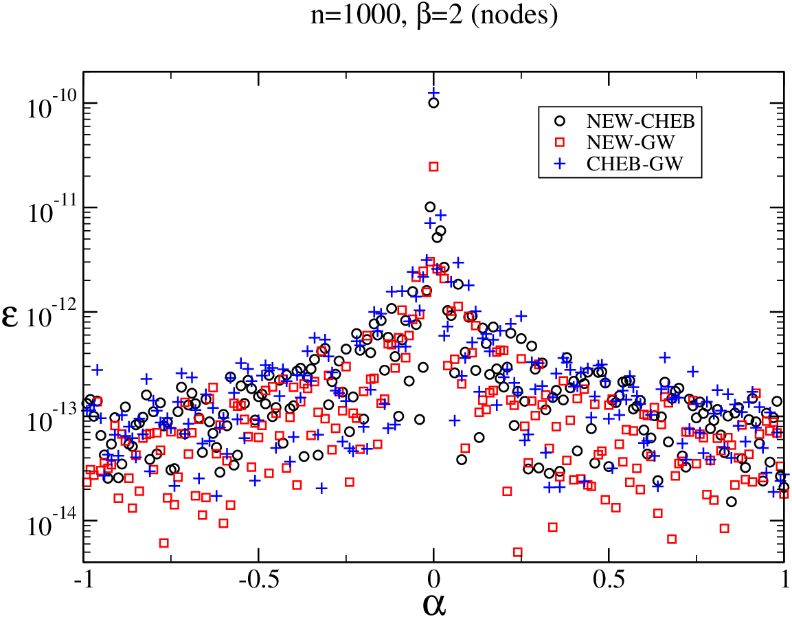
In Fig. 4 we plot the relative maximum accuracy for the weights obtained for Gauss–Jacobi quadrature with parameters and comparing the three different pairs of methods NEW–CHEB, NEW–GW and CHEB–GW, and for three values of : (when CHEB uses recurrences for computing the polynomials), (when CHEB uses asymptotics) and (again, CHEB uses asymptotics). In addition, we also show the maximum relative accuracy for the nodes in the case and for the same values of and .
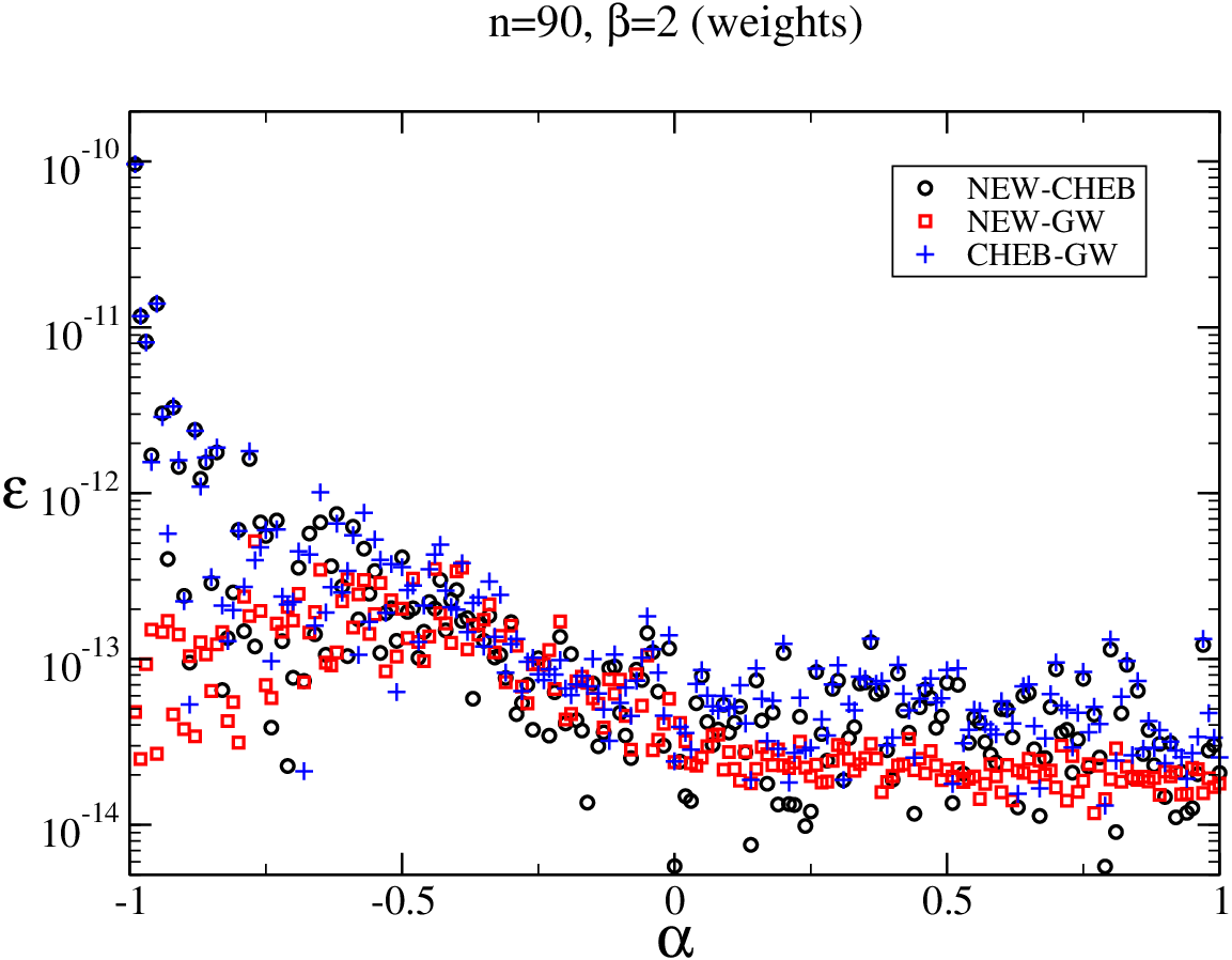
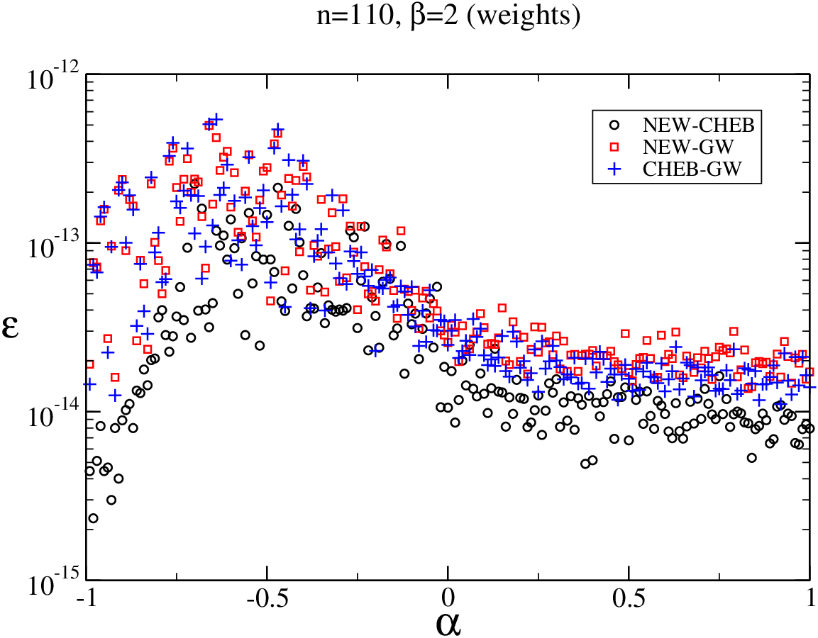
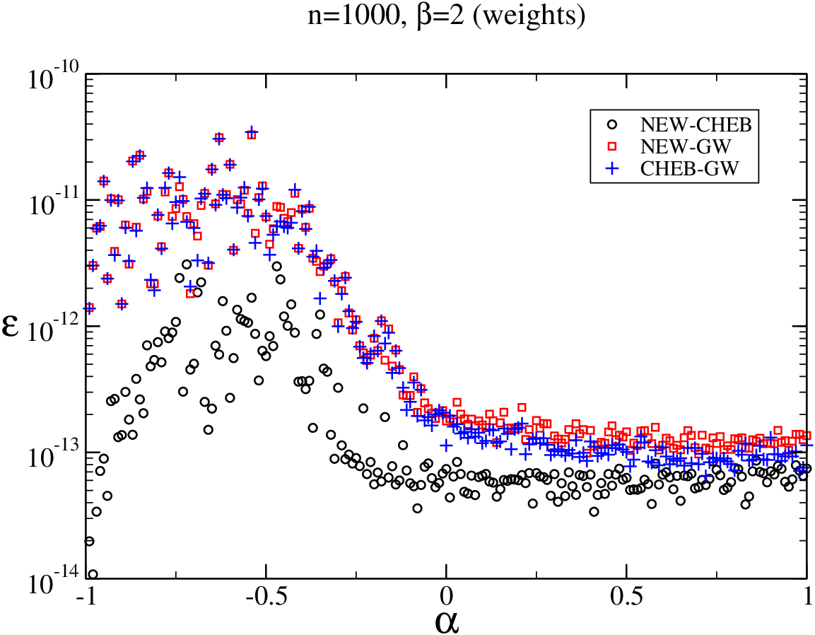
For , the relative maximum error for the weights is very similar for the three comparisons except that as the error for the NEW–GW comparison is smaller; this suggests that CHEB loses some accuracy in this limit. The same behavior is observed for the symmetrical cases and we have checked with our quadruple precision Fortran program that the most accurate method in this limit is NEW.
For CHEB uses asymptotics to compute the polynomials and in this case the accuracy of the weights appears to be close to double precision accuracy (as checked in the symmetric case by comparing with our quadruple precision Fortran program). We observe in this case that the error worsens for negative and in particular close to ; for such values the comparison is favorable for NEW with respect to GW and we conclude that the most accurate method is CHEB, followed by NEW and the less accurate is GW. We stress again that whenever a faster and more accurate method is that of Gil:2019:NIC, with close to double precision accuracy for the nodes and weights. The case for the weights in Fig. 4 shows similar results as for .
Finaly, in Fig. 4 (bottom, right) we show a plot of the maximum relative error in the computation of the nodes when . The method NEW is able to compute the nodes with full double precision accuracy and for any ; differently, CHEB and GW do not compute the nodes with relative accuracy, but with absolute accuracy, which means that there is some relative error degradation for the nodes closer to as increases. For the case shown, this error degradation is more noticeable for close to zero because nodes close to occur. We have repeated these tests for other values of and and we conclude that the error degradation for the nodes scales as for CHEB and as for GW.
5.2.3 Comparing against a higher precision algorithm
In order to confirm the information that we have extracted by intensive comparison tests between three different methods implemented in double precision (with Matlab), we have also compared the outputs of the NEW and CHEB methods against a high accuracy computation; for this purpose, we have implemented the Golub-Welsch algorithm in Maple. These tests are, necessarily, more time consuming and less extensive, and the values of are more limited (for instance the tests for with Maple are impractical), but we use them to illustrate the behaviour of the relative errors for each node and weight.
In Fig. 5 we show relative errors for the weights. The absolute errors can of course be easily obtained from the relative errors by multiplying them by the values of the weights (which for large enough could be estimated with Eq. (15)).


The top graphs in Fig. 5 display the relative error in the computation of each weight for and several values of ; in the up left figure (when the polynomials are computed by recursion in CHEB), while in the up right figure (with polynomials computed by asymptotics in CHEB). The errors for NEW are ploted in black, while the CHEB errors are plotted in blue. In the up left figure, we observe that CHEB is able to provide typically one additional digit of accuracy with respect to NEW for most the weights; the exception to this is found on the weights corresponding to the largest nodes (which are the largest weights for and , as it is easy to check using Eq. (15)). In particular, we observe a degradation of accuracy as in CHEB and the relative error for the largest weight for , and is (this point is not shown in the graph in order to improve the visibility of the rest of the graph). In the tests corresponding to this up left figure, we used Maple with 40 digits in the computation of the Goulb-Welsch algorithm.
In the up right figure, we observe that the relative accuracy for CHEB has improved in relation to NEW with respect to the case , and that, again, some accuracy loss happens for the largest weights. For these values of , it seems more convenient to use methods based on asymptotics for computing the weights when they are available as is the case of CHEB (using Newton iterations) and also of the methods in Gil:2019:NIC (without Newton iterations).
The bottom-left graph in Fig. 5 shows one case for which asymptotic methods are not available, and for which NEW does produce accurate results. For these large values of the parameters, the smallest weights are many orders of magnitude larger that the largest weights, and for this reason at least 140 digits of accuracy are needed in Maple in order to compute the weights with the Golub-Welsch algorithm, while NEW only requires 15-16 digits.
We summarize in Tables 2-4 the maximum relative and relative maximum errors for the weights for the parameters considering in Fig. 5. We observe that when the maximum relative error is equal to the relative maximum errot this means that the relative error reaches its maximum value for the most significant weight.
Finally, regarding the errors for the nodes, the absolute errors both fo NEW and CHEB are close to and therefore consistent with double precision accuracy (the resulting noisy graph is not very interesting and it is not shown). The difference between the NEW and CHEB methods is that, as commented before, CHEB computes the nodes with absolute double precision accuracy but not relative accuracy, which results in some degradation of relative accuracy for the nodes close to zero. This is shown in Fig. 5 bottom-right. For NEW the relative accuracy is found to be better than and is not shown.
As a way of summary, each method has its advantages in terms of accuracy. The main novelty of NEW is that the range of parameters available is drastically increased and that, being a method based on finite or convergent processes, it can be extended to arbitrary accuracy (as illustrated with the Gauss-Gegenbauer case). Apart from this, as we will see next, the method turns out to be very efficient.
An optimal algorithm for computing Gauss quadrature rules should combine the use of asymptotic methods (when available) with the use of fully convergent methods capable of high accuracy computations, like the one we have presented. A full and extensive accuracy test of the available methods as a function of the three parameters is outside the scope of the present paper.
|
|
|
5.3 CPU times
In Fig. 6 we compare the CPU time spent by the methods NEW, CHEB and GW as a function of the degree and for several values of and .
We observe that the behavior of the methods NEW and GW does not change much for the three cases shown (Gauss–Legendre, Gauss–Gegenbauer with and Gauss–Jacobi with , ), while for CHEB there are significant differences, because CHEB uses different methods depending on the value of the parameters and the degree.
For the case of Gauss–Legendre, CHEB uses the asymptotic approximations of Bogaert:2014:IFC when and computation of Legendre polynomials through recurrence for ; in this case, we observe that CHEB is the fastest method. This could be expected because for direct asymptotics are used, without iterative methods, and for the simplified expressions for the Legendre case are also faster to compute. Except for , where GW appears to be faster, CHEB appears to be preferable.
For the Gauss–Gegenbauer case shown, CHEB uses the iterative method based on asymptotics for and computation used on recurrences otherwise; this is observed in the jump in CPU times for , and NEW becomes faster in this case. For smaller the performance are more or less close to each other. For smaller values of () the results are quite similar to the next case we discuss (Gauss–Jacobi), because in this case CHEB uses iteration based on asymptotics for (results not shown).
Finally, for the most general non-symmetric cases, the advantage of NEW in terms of speed becomes clear (Fig. 5 bottom, left) and only GW is faster for . Therefore, except for the symmetric cases, the algorithm NEW is faster.
Even without making specific algorithms for the symmetric cases in our Matlab implementation, it is competitive to CHEB in that cases, and clearly faster for non symmetric cases. In order to show this we plot the ratio of the CPU times between the CHEB and NEW methods (Fig. 5, bottom, right). We show these ratios, as a function of , for four cases: Gauss–Legendre, two Gauss–Gegenbauer cases and Gauss–Jacobi example. Our method, except for the Legendre case for large , is competitive when it is not faster.


Appendix A: On the conditioning of the recurrence for computing derivatives.
We briefly discuss the conditioning of the computation of the derivatives with the recurrence relation (26). This is a five term recurrence relation, with a space of solutions of dimension four. For studying the conditioning as we can divide all terms of the recurrence by and then all the coefficients have finite limit as . We have
with
Then it is known (see for instance Elaydi:2005:AIT, Theorem 8.11) that the solutions of the recurrence satisfy
| (45) |
where is the modulus of one of the solutions of the characteristic polynomial
which, upon dividing by and denoting we can write
And because is a polynomial of degree four () this equation is the same as , which, solving for gives two double roots . This means that the possible values of in Eq. (45) are and and there is a subspace of dimension satisfying (45) with and a second subspace with ; the first space will be dominant over the second when and the opposite when (the case is the degenerate case, in which no solution is exponentially dominant over the rest).
In our case, we have with given by (10). We notice that for and odd, is a polynomial of degree , and then if . The Taylor series have a finite number of terms in this case and the analysis of stability for as is not needed. Let us now consider that neither nor are odd, and we leave for later the case in which only one of the parameters ( or ) is odd.
When neither nor are odd, then Taylor series at has an infinite number of terms. Because is a polynomial times the radius of convergence of the series for centered at ,
is (which we could expect because the ODE satisfied by has singularities at ) and then
Therefore in this case the sequence , is in the dominant subspace of solutions of the recurrence.
The case when either or is odd but not both is different. Let us for instance consider that is odd, but not . In this case, the convergence of the series is limited by the singularity at (but not at ); the radius of convergence in this case is therefore and then
Therefore, is in the dominant subspace only if . In this case for large enough the forward computation of would be unstable for positive . However, even for this case we have not observed inaccuracies in the computation of the series. For a given accuracy claim, the number of terms in the series needed are not high enough to produce stability issues.
Acknowledgements.
NMT thanks CWI for scientific support.References
- (1) Bogaert, I.: Iteration-free computation of Gauss-Legendre quadrature nodes and weights. SIAM J. Sci. Comput. 36(3), A1008–A1026 (2014). DOI 10.1137/140954969. URL http://dx.doi.org/10.1137/140954969
- (2) Bogaert, I., Michiels, B., Fostier, J.: O(1) computation of Legendre polynomials and Gauss-Legendre nodes and weights for parallel computing. SIAM J. Sci. Comput. 34(3), C83–C101 (2012). DOI 10.1137/110855442. URL http://dx.doi.org/10.1137/110855442
- (3) Bremer, J., Yang, H.: Fast algorithms for Jacobi expansions via nonoscillatory phase functions. IMA J. Numer. Anal. 40(3), 2019–2051 (2020). DOI 10.1093/imanum/drz016. URL https://doi.org/10.1093/imanum/drz016
- (4) Davis, P.J., Rabinowitz, P.: Some geometrical theorems for abscissas and weights of Gauss type. J. Math. Anal. Appl. 2, 428–437 (1961). DOI 10.1016/0022-247X(61)90021-X. URL https://doi.org/10.1016/0022-247X(61)90021-X
- (5) Deaño, A., Gil, A., Segura, J.: New inequalities from classical Sturm theorems. J. Approx. Theory 131(2), 208–230 (2004). DOI 10.1016/j.jat.2004.09.006. URL https://doi.org/10.1016/j.jat.2004.09.006
- (6) Deaño, A., Segura, J.: Global Sturm inequalities for the real zeros of the solutions of the Gauss hypergeometric differential equation. J. Approx. Theory 148(1), 92–110 (2007). DOI 10.1016/j.jat.2007.02.005. URL https://doi.org/10.1016/j.jat.2007.02.005
- (7) Driscoll, T.A., Hale, N., Trefethen, L.N.: Chebfun Guide. Pafnuty Publications, Oxford (2014)
- (8) Elaydi, S.: An introduction to difference equations, third edn. Undergraduate Texts in Mathematics. Springer, New York (2005)
- (9) Gil, A., Segura, J., Temme, N.M.: Asymptotic expansions of Jacobi polynomials and of the nodes and weights of Gauss-Jacobi quadrature for large degree and parameters in terms of elementary functions. Submitted. URL https://arxiv.org/abs/2007.10748
- (10) Gil, A., Segura, J., Temme, N.M.: Numerical methods for special functions. Society for Industrial and Applied Mathematics (SIAM), Philadelphia, PA (2007). DOI 10.1137/1.9780898717822
- (11) Gil, A., Segura, J., Temme, N.M.: Numerically satisfactory solutions of hypergeometric recursions. Math. Comp. 76(259), 1449–1468 (2007). DOI 10.1090/S0025-5718-07-01918-7. URL https://doi.org/10.1090/S0025-5718-07-01918-7
- (12) Gil, A., Segura, J., Temme, N.M.: GammaCHI: a package for the inversion and computation of the gamma and chi-square cumulative distribution functions (central and noncentral). Comput. Phys. Commun. 191, 132–139 (2015). DOI 10.1016/j.cpc.2015.01.004. URL https://doi.org/10.1016/j.cpc.2015.01.004
- (13) Gil, A., Segura, J., Temme, N.M.: Asymptotic approximations to the nodes and weights of Gauss-Hermite and Gauss-Laguerre quadratures. Stud. Appl. Math. 140(3), 298–332 (2018). DOI 10.1111/sapm.12201. URL https://doi.org/10.1111/sapm.12201
- (14) Gil, A., Segura, J., Temme, N.M.: Fast, reliable and unrestricted iterative computation of Gauss–Hermite and Gauss–Laguerre quadratures. Numer. Math. 143(3), 649–682 (2019). DOI 10.1007/s00211-019-01066-2. URL https://doi.org/10.1007/s00211-019-01066-2
- (15) Gil, A., Segura, J., Temme, N.M.: Noniterative computation of Gauss-Jacobi quadrature. SIAM J. Sci. Comput. 41(1), A668–A693 (2019). DOI 10.1137/18M1179006. URL https://doi.org/10.1137/18M1179006
- (16) Glaser, A., Liu, X., Rokhlin, V.: A fast algorithm for the calculation of the roots of special functions. SIAM J. Sci. Comput. 29(4), 1420–1438 (2007). DOI 10.1137/06067016X. URL http://dx.doi.org/10.1137/06067016X
- (17) Golub, G.H., Welsch, J.H.: Calculation of Gauss quadrature rules. Math. Comp. 23 (1969), 221-230; addendum, ibid. 23(106, loose microfiche suppl), A1–A10 (1969)
- (18) Hale, N., Townsend, A.: Fast and accurate computation of Gauss-Legendre and Gauss-Jacobi quadrature nodes and weights. SIAM J. Sci. Comput. 35(2), A652–A674 (2013). DOI 10.1137/120889873. URL http://dx.doi.org/10.1137/120889873
- (19) Johansson, F., Mezzarobba, M.: Fast and rigorous arbitrary-precision computation of Gauss-Legendre quadrature nodes and weights. SIAM J. Sci. Comput. 40(6), C726–C747 (2018). DOI 10.1137/18M1170133. URL https://doi.org/10.1137/18M1170133
- (20) Koornwinder, T.H., Wong, R., Koekoek, R., Swarttouw, R.F.: Orthogonal polynomials. In: NIST handbook of mathematical functions, pp. 435–484. U.S. Dept. Commerce, Washington, DC (2010)
- (21) Opsomer, P.: Asymptotics for Orthogonal Polynomials and High-frequency Scattering Problems. PhD thesis, KU Leuven (2018). URL https://lirias.kuleuven.be/retrieve/493748
- (22) Segura, J.: Reliable computation of the zeros of solutions of second order linear ODEs using a fourth order method. SIAM J. Numer. Anal. 48(2), 452–469 (2010). DOI 10.1137/090747762. URL http://dx.doi.org/10.1137/090747762
- (23) Swarztrauber, P.N.: On computing the points and weights for Gauss-Legendre quadrature. SIAM J. Sci. Comput. 24(3), 945–954 (electronic) (2002). DOI 10.1137/S1064827500379690. URL http://dx.doi.org/10.1137/S1064827500379690
- (24) Trefethen, L.N.: Is Gauss quadrature better than Clenshaw-Curtis? SIAM Rev. 50(1), 67–87 (2008). DOI 10.1137/060659831. URL https://doi.org/10.1137/060659831
- (25) Yakimiw, E.: Accurate computation of weights in classical Gauss-Christoffel quadrature rules. J. Comput. Phys. 129(2), 406–430 (1996). DOI 10.1006/jcph.1996.0258. URL http://dx.doi.org/10.1006/jcph.1996.0258