跳到论文正文
W Papers独立论文阅读器 arXiv:2008.08489 论文正文 计算阅读时间 · 0%
引用这篇论文根据当前论文元数据生成,正式投稿前建议核对。


License: arXiv.org perpetual non-exclusive license
arXiv:2008.08489v4 [math-ph] 17 May 2021

Mathematics of magic angles
in a model of twisted bilayer graphene

Simon Becker Email address: simon.becker@damtp.cam.ac.uk Address: Department of Applied Mathematics and Theoretical Physics, University of Cambridge, Wilberforce Road, Cambridge, CB3 0WA, United Kingdom. , Mark Embree Email address: embree@vt.edu Address: Department of Mathematics, Virginia Tech, Blacksburg, VA 24061, USA , Jens Wittsten Email address: jens.wittsten@math.lu.se Address: Centre for Mathematical Sciences, Lund University, Box 118, SE-221 00 Lund, Sweden, and Department of Engineering, University of Borås, SE-501 90 Borås, Sweden and Maciej Zworski Email address: zworski@math.berkeley.edu Address: Department of Mathematics, University of California, Berkeley, CA 94720, USA.
Abstract.

We provide a mathematical account of the recent Physical Reviews Letter by Tarnopolsky–Kruchkov–Vishwanath [TKV19]. The new contributions are a spectral characterization of magic angles, its accurate numerical implementation and an exponential estimate on the squeezing of all bands as the angle decreases. Pseudospectral phenomena [DSZ04],[TrEm05], due to the non-hermitian nature of operators appearing in the model considered in [TKV19] play a crucial role in our analysis.

1. Introduction and statement of results

Figure 1. Reciprocals of magic angles for the specific potential (1.2): resonant α\alpha’s (red circles) come from the full spectrum of the compact operator (1.9) defining magic angles, and the magic α\alpha’s (black dots) are the reciprocals of the “physically relevant” positive angles.

Following a recent Physical Review Letter by Tarnopolsky–Kruchkov–Vishwanath [TKV19] we consider the following Hamiltonian modeling twisted bilayer graphene:

H⁡(α):=(0D​(α)∗D⁡(α)0),D⁡(α):=(2​Dz¯α​U​(z)α​U​(−z)2​Dz¯),H(\alpha):=\begin{pmatrix}0&D(\alpha)^{*}\\ D(\alpha)&0\end{pmatrix},\ \ \ D(\alpha):=\begin{pmatrix}{2}D_{\bar{z}}&\alpha U(z)\\ \alpha U(-z)&{2}D_{\bar{z}}\end{pmatrix}, (1.1)

where z=x1+i​x2z=x_{1}+ix_{2}, Dz¯:=12​i(∂x1+i∂x2)D_{\bar{z}}:=\tfrac{1}{2i}(\partial_{x_{1}}+i\partial_{x_{2}}) and

U⁡(z)=U⁡(z,z¯):=∑k=02ωk​e12​(z​ω¯k−z¯​ωk),ω:=e2​π​i/3.U(z)=U(z,\bar{z}):=\sum_{k=0}^{2}\omega^{k}e^{\frac{1}{2}(z\bar{\omega}^{k}-\bar{z}\omega^{k})},\ \ \ \omega:=e^{2\pi i/3}. (1.2)

(We abuse the notation in the argument of UU for the sake of brevity and write U⁡(z)U(z) rather than U⁡(z,z¯)U(z,\bar{z}).) The dimensionless parameter α\alpha is essentially the reciprocal of the angle of twisting between the two layers. When two honeycomb lattices are twisted against one another, a periodic honeycomb superlattice, called the moiré lattice, becomes visible. (This name comes from the patterns formed when two fabrics lie on top of each other.) Bistritzer and MacDonald in [BiMa11] predicted that the symmetries of the periodic moiré lattice lead to dramatic flattening of the band spectrum. The operator (1.1) and in particular potential (1.2) were obtained in [TKV19] by removing certain interaction terms from the operator constructed in [BiMa11].

In this paper we consider any potential having the symmetries of (1.2):

𝐚=43πiωℓ,ℓ=1,2⟹U(z+𝐚)=ω¯U(z), and U⁡(ω​z)=ω​U​(z).\begin{gathered}\mathbf{a}=\tfrac{4}{3}\pi i\omega^{\ell},\ \ell=1,2\ \Longrightarrow\ U(z+\mathbf{a})=\bar{\omega}U(z),\text{ and }\\ U(\omega z)=\omega U(z).\end{gathered} (1.3)

The only exception is Theorem 4 which requires a non-triviality assumption, see (4.3). Such potentials are explored further in Section 4.

The Hamiltonian HH is periodic with respect to a lattice Γ\Gamma (see (2.2) below) and magic angles are defined as the α\alpha’s (or rather their reciprocals) at which

0∈⋂𝐤∈ℂSpecL2​(ℂ/Γ)⁡(H𝐤​(α)),H𝐤​(α):=(0D​(α)∗−𝐤¯D⁡(α)−𝐤0).0\in\bigcap_{\mathbf{k}\in{\mathbb{C}}}\Spec_{L^{2}({\mathbb{C}}/\Gamma)}(H_{\mathbf{k}}(\alpha)),\ \ \ H_{\mathbf{k}}(\alpha):=\begin{pmatrix}0&D(\alpha)^{*}-\bar{\mathbf{k}}\\ D(\alpha)-\mathbf{k}&0\end{pmatrix}. (1.4)

The Hamiltonian H𝐤​(α)H_{\mathbf{k}}(\alpha) comes from the Floquet theory of H⁡(α)H(\alpha) and (1.4) means that H⁡(α)H(\alpha) has a flat band at 00 (see Proposition 2.4 below). Since the Bloch electrons have the same energy at the flat bands, strong electron-electron interactions leading to effects such as superconductivity have been observed at magic angles. We refer to [TKV19] for physical motivation and references. Some aspects of this paper carry over to more general models such as the Bistritzer–MacDonald [BiMa11] and that is discussed in [B*21].

The first theorem is, essentially, the main mathematical result of [TKV19]. To formulate it we define the Wronskian of two ℂ2{\mathbb{C}}^{2}-valued Γ\Gamma-periodic functions:

W⁡(𝐮,𝐯)=det[𝐮,𝐯],𝐮,𝐯∈ℂ2,W(\mathbf{u},\mathbf{v})=\det[\mathbf{u},\mathbf{v}],\ \ \ \mathbf{u},\mathbf{v}\in{\mathbb{C}}^{2}, (1.5)

noting that if D⁡(α)​𝐮=D⁡(α)​𝐯=0D(\alpha)\mathbf{u}=D(\alpha)\mathbf{v}=0, then WW is constant (applying ∂z¯\partial_{\bar{z}} shows that WW is holomorphic and periodic). We also define an involution ℰ\mathscr{E} satisfying ℰ​D​(α)=D⁡(α)​ℰ\mathscr{E}D(\alpha)=D(\alpha)\mathscr{E}:

ℰ​𝐮​(α,z):=(0−11 0)​𝐮​(α,−z).\mathscr{E}\mathbf{u}(\alpha,z):=\begin{pmatrix}0&-1\\ 1&\ \ 0\end{pmatrix}\mathbf{u}(\alpha,-z). (1.6)

We then have

Theorem 1.

Suppose that D⁡(α)D(\alpha) is given by (1.1) with U∈C∞​(ℂ/Γ,ℂ)U\in C^{\infty}({\mathbb{C}}/\Gamma;{\mathbb{C}}) satisfying (1.3). Then there exists a real-analytic function ff on ℝ{\mathbb{R}} such that

0∈⋂𝐤∈ℂSpecL2​(ℂ/Γ)⁡(H𝐤​(α))⟺f⁡(α)=0.0\in\bigcap_{\mathbf{k}\in{\mathbb{C}}}\Spec_{L^{2}({\mathbb{C}}/\Gamma)}(H_{\mathbf{k}}(\alpha))\ \Longleftrightarrow f(\alpha)=0.

The function ff is defined using a projectively unique family ℝ∋α↦𝐮⁡(α)∈C∞​(ℂ/Γ,ℂ2){\mathbb{R}}\ni\alpha\mapsto\mathbf{u}(\alpha)\in C^{\infty}({\mathbb{C}}/\Gamma;{\mathbb{C}}^{2}) such that 𝐮⁡(0)=(1,0)t\mathbf{u}(0)=(1,0)^{t}, D⁡(α)​𝐮​(α)=0D(\alpha)\mathbf{u}(\alpha)=0. Then f⁡(α):=W⁡(𝐮⁡(α),ℰ​𝐮​(α))f(\alpha):=W(\mathbf{u}(\alpha),\mathscr{E}\mathbf{u}(\alpha)), where WW is given by (1.5) and ℰ\mathscr{E} is defined in (1.6).

Refer to caption
Figure 2. For Uμ​(z)=U⁡(z)+μ​∑k=02ωk​ez¯​ωk−z​ω¯kU_{\mu}(z)=U(z)+\mu\sum_{k=0}^{2}\omega^{k}e^{\bar{z}\omega^{k}-z\bar{\omega}^{k}}, with UU given by (1.2) and μ=−1.96\mu=-1.96, we show set 𝒜\mathcal{A} (indicated by ∙\bullet). The distribution is much less regular than for μ=0\mu=0 shown in Figure 1, and nothing like (1.12) can be expected. The coloured paths trace the dynamics of magic α\alpha’s for −2.2≤μ≤−1.7-2.2\leq\mu\leq-1.7: to understand the dependence of “physically relevant” real α\alpha’s complex values should be considered.

A more precise, representation theoretical, description of 𝐮⁡(α)\mathbf{u}(\alpha) will be given in §2. Projective uniqueness means uniqueness up to a multiplicative factor. In §3 we show that (after possibly switching 𝐮\mathbf{u} and ℰ​𝐮\mathscr{E}\mathbf{u})

v⁡(α):=W⁡(𝐮⁡(α),ℰ​𝐮​(α))=0⟺𝐮⁡(α,zS)=0,zS:=4​39​π,v(\alpha):=W(\mathbf{u}(\alpha),\mathscr{E}\mathbf{u}(\alpha))=0\ \Longleftrightarrow\ \mathbf{u}(\alpha,z_{S})=0,\ \ \ z_{S}:=\tfrac{4\sqrt{3}}{9}\pi, (1.7)

which then provides a recipe [TKV19] for constructing the zero eigenfunctions of H𝐤​(α)H_{\mathbf{k}}(\alpha): if v⁡(α)=0v(\alpha)=0 then (D⁡(α)−𝐤)​𝐮𝐤​(α)=0(D(\alpha)-\mathbf{k})\mathbf{u}_{\mathbf{k}}(\alpha)=0, 𝐮𝐤​(α)∈C∞​(ℂ/Γ,ℂ2)\mathbf{u}_{\mathbf{k}}(\alpha)\in C^{\infty}({\mathbb{C}}/\Gamma;{\mathbb{C}}^{2}), where

𝐮𝐤​(z)=ei2​(z​𝐤¯+z¯​𝐤)​θ−16+k1/3,16−k2/3​(3​z/4​π​i​ω|ω)θ−16,+16​(3​z/4​π​i​ω|ω)​𝐮​(z),𝐤=13​(k1​ω2−k2​ω),\mathbf{u}_{\mathbf{k}}(z)=e^{\frac{i}{2}(z\bar{\mathbf{k}}+\bar{z}{\mathbf{k}})}\frac{\theta_{-\frac{1}{6}+k_{1}/3,\frac{1}{6}-k_{2}/3}(3z/4\pi i\omega|\omega)}{\theta_{-\frac{1}{6},+\frac{1}{6}}(3z/4\pi i\omega|\omega)}\mathbf{u}(z),\ \ \mathbf{k}=\tfrac{1}{\sqrt{3}}(k_{1}\omega^{2}-k_{2}\omega), (1.8)

where ζ↦θa,b​(ζ|ω)\zeta\mapsto\theta_{a,b}(\zeta|\omega) is the Jacobi theta function – see §3.2 for a brief review and [Mu83, Chapter I] for a proper introduction. (Our convention is slightly different than that in [TKV19] but the formulas are equivalent.)

The next theorem provides a simple spectral characterization of α\alpha’s satisfying (1.4). Combined with some symmetry reductions (see §§2,5) this characterization allows a precise calculation of the leading magic α\alpha’s – see Table 1 for the values of the first 13 elements of 𝒜mag\mathcal{A}_{\rm{mag}} and Tables 2, 3 for rigorous error bounds. As seen in Proposition 5.2, it also implies that the multiplicities of flat bands at 00 is at least 18.

Refer to caption
Refer to caption
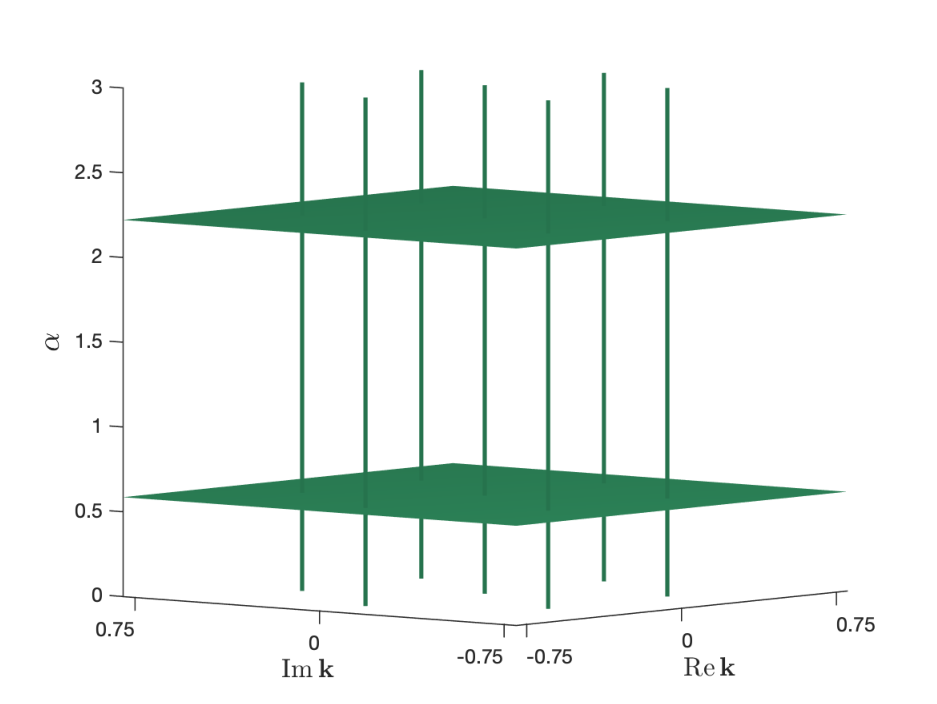
Figure 3. Left: spectrum of D⁡(α)D(\alpha) as α\alpha varies. Right: level surface of 𝐤↦‖(D⁡(α)−𝐤)−1‖=102\mathbf{k}\mapsto\|(D(\alpha)-\mathbf{k})^{-1}\|=10^{2} as α\alpha varies: we see that the norm of the resolvent (D⁡(α)−𝐤)−1(D(\alpha)-\mathbf{k})^{-1} grows as we approach the first two magic α\alpha’s (near 0.5860.586 and 2.2212.221), at which it blows up for all kk. In any discretization that norm would be finite except on a finite set but it would blow up as the discretization improves.
Theorem 2.

Let Γ∗\Gamma^{*} be the dual lattice and define the family of compact operators

T𝐤:=(2​Dz¯−𝐤)−1​(0U⁡(z)U⁡(−z)0),𝐤∉Γ∗,T_{\mathbf{k}}:=(2D_{\bar{z}}-\mathbf{k})^{-1}\begin{pmatrix}0&U(z)\\ U(-z)&0\end{pmatrix},\ \ \mathbf{k}\notin\Gamma^{*}, (1.9)

where U⁡(z)U(z) is given by (1.2), or more generally satisfies U∈C∞​(ℂ/Γ,ℂ)U\in C^{\infty}({\mathbb{C}}/\Gamma;{\mathbb{C}}) and (1.3). Then the spectrum of T𝐤T_{\mathbf{k}} is independent of 𝐤∉Γ∗\mathbf{k}\notin\Gamma^{*}, and the following statements are equivalent:

  1. (1)

    1/α∈SpecL2​(ℂ/Γ)⁡(T𝐤),𝐤∉Γ∗1/\alpha\in\Spec_{L^{2}({\mathbb{C}}/\Gamma)}(T_{\mathbf{k}}),\ \ \mathbf{k}\notin\Gamma^{*};

  2. (2)

    SpecL2​(ℂ/Γ)⁡D⁡(α)=ℂ\Spec_{L^{2}({\mathbb{C}}/\Gamma)}D(\alpha)={\mathbb{C}} ;

  3. (3)

    0∈⋂𝐤∈ℂSpecL2​(ℂ/Γ)⁡(H𝐤​(α))0\in\bigcap_{\mathbf{k}\in{\mathbb{C}}}\Spec_{L^{2}({\mathbb{C}}/\Gamma)}(H_{\mathbf{k}}(\alpha)), where H𝐤H_{\mathbf{k}} is defined in (1.4).

We denote the full set of resonant α\alpha’s and the set of magic α\alpha’s as

𝒜:=1/(SpecL2​(ℂ/Γ)(T𝐤)∖{0}),𝐤∉Γ∗,𝒜mag:=𝒜∩(0,∞)={αj}j≥1,α1<α2<⋯,\begin{gathered}\mathcal{A}:=1/(\Spec_{L^{2}({\mathbb{C}}/\Gamma)}(T_{\mathbf{k}})\setminus\{0\}),\ \ \mathbf{k}\notin\Gamma^{*},\\ \kern 6.25pt\mathcal{A}_{\rm{mag}}:=\mathcal{A}\cap(0,\infty)=\{\alpha_{j}\}_{j\geq 1},\ \ \alpha_{1}<\alpha_{2}<\cdots,\end{gathered} (1.10)

respectively. The elements of 𝒜\mathcal{A} are included with their multiplicities as multiplicities of eigenvalues of T𝐤T_{\mathbf{k}}. Those multiplicities are at least 99 – see Proposition 5.2. Numerical evidence suggests that multiplicities of 𝒜mag\mathcal{A}_{\rm{mag}} are exactly 99 and that is related to the question about zeros of u⁡(α)u(\alpha) – see (1.7) and Remark 1 after Proof of Theorem 1 in §3.

As a simple byproduct of Theorems 1 and 2 we have

SpecL2​(ℂ/Γ)⁡D⁡(α)=Γ∗,α∉𝒜.\Spec_{L^{2}({\mathbb{C}}/\Gamma)}D(\alpha)=\Gamma^{*},\ \ \alpha\notin\mathcal{A}.

Examples of operators which have either discrete spectra or all of ℂ{\mathbb{C}} as spectrum, depending on analytic variation of coefficients, have been known before, see for instance Seeley [Se86]. The operator D⁡(α)D(\alpha) provides a new striking example of such phenomena, showing that it is physically relevant and not merely pathological.

If we assume that U⁡(z)=U⁡(z¯)¯U(z)=\overline{U(\bar{z})}, then Proposition 3.2 below (see also Figure 1) also gives 𝒜=−𝒜=𝒜¯\mathcal{A}=-\mathcal{A}=\overline{\mathcal{A}}.

Mathematical description of 𝒜\mathcal{A} remains open and here we only contribute the following simple result:

Theorem 3.

For the potential UU given by (1.2) we have

∑α∈𝒜α−4=72​π/3,\sum_{\alpha\in\mathcal{A}}\alpha^{-4}={72\pi}/{\sqrt{3}}, (1.11)

where α\alpha’s are included according to their multiplicities. In particular, 𝒜≠∅\mathcal{A}\neq\emptyset.

Figure 4. On the left, the smallest non-negative eigenvalues of H𝐤​(α)H_{\mathbf{k}}(\alpha), α=5\alpha=5, 𝐤=k​ω/3\mathbf{k}=k\omega/\sqrt{3}, −12≤k≤12-\frac{1}{2}\leq k\leq\frac{1}{2}. On the right, E0​(𝐤,α)E_{0}({\mathbf{k}},\alpha) (log scale) for several values 𝐤\mathbf{k}. (The point 𝐤=1/(2​3)+i/6{\mathbf{k}}=1/(2\sqrt{3})+i/6 is farthest from an eigenvalue of D⁡(α)D(\alpha) for α∉𝒜\alpha\not\in{\mathcal{A}}.) The exponential squeezing of the bands described in Theorem 4 is clearly visible.

Concerning 𝒜mag\mathcal{A}_{\rm{mag}}, an intriguing asymptotic relation for αj\alpha_{j}’s for UU given by (1.2) was suggested by the numerics in [TKV19]:

αj+1−αj≃32,j≫1.\alpha_{j+1}-\alpha_{j}\simeq\tfrac{3}{2},\ \ j\gg 1. (1.12)

We do not address this problem here except numerically in §5 and in Figure 2, which shows that regular spacing does not hold for general potentials. The following result based on Dencker–Sjöstrand–Zworski [DSZ04] indicates the mathematical subtlety underlying the distribution problem: for large values of α\alpha the bands get exponentially squeezed, making it difficult to find the ones that are exactly zero; see Figure 4 and the following

Theorem 4.

Suppose that H𝐤​(α)H_{\mathbf{k}}(\alpha) is given by (1.1) and (1.4) with UU given by (1.2) and that

SpecL2​(ℂ/Γ)⁡H𝐤​(α)={Ej​(𝐤,α)}j∈ℤ,Ej​(𝐤,α)≤Ej+1​(𝐤,α),𝐤∈ℂ,α>0,\Spec_{L^{2}({\mathbb{C}}/\Gamma)}H_{\mathbf{k}}(\alpha)=\{E_{j}(\mathbf{k},\alpha)\}_{j\in{\mathbb{Z}}},\ \ \ E_{j}(\mathbf{k},\alpha)\leq E_{j+1}(\mathbf{k},\alpha),\ \ \mathbf{k}\in{\mathbb{C}},\ \ \alpha>0,

with the convention that E0​(𝐤,α)=minj⁡|Ej​(𝐤,α)|E_{0}(\mathbf{k},\alpha)=\min_{j}|E_{j}(\mathbf{k},\alpha)|. Then there exist positive constants c0c_{0}, c1c_{1}, and c2c_{2} such that for all 𝐤∈ℂ\mathbf{k}\in{\mathbb{C}},

|Ej​(𝐤,α)|≤c0​e−c1​α,|j|≤c2​α,α>0.|E_{j}(\mathbf{k},\alpha)|\leq c_{0}e^{-c_{1}\alpha},\ \ |j|\leq c_{2}\alpha,\ \ \alpha>0. (1.13)

Numerical experiments presented in Figure 7 (see also Figure 4) suggest that for any c2c_{2} there exists c0c_{0} for which (1.13) holds, with c1=1c_{1}=1. The theorem is proved by showing that for large α\alpha every point “wants to be” in the spectrum of D⁡(α)D(\alpha) modulo an exponentially small error. That is a typical pseudospectral effect in the study of non-hermitian operators – see Trefethen–Embree [TrEm05] for a broad description of such phenomena. Although H𝐤​(α)H_{\mathbf{k}}(\alpha) is self-adjoint, having a zero eigenvalue is equivalent to 𝐤∈SpecL2​(ℂ/Γ)⁡(D⁡(α))\mathbf{k}\in\Spec_{{L^{2}({\mathbb{C}}/\Gamma)}}(D(\alpha)) and D⁡(α)D(\alpha) is highly non-normal. This is illustrated in Figure 3. In Section 4 we explore the situation for general potentials satisfying the symmetries (1.3), and prove that a result corresponding to Theorem 4 continues to hold if an additional non-triviality assumption is imposed; see (4.3) and Theorem 5. (Some condition is clearly needed, as shown by the example of U≡0U\equiv 0.)

Watson and Luskin [WaLu21] have recently provided an alternative proof of Theorem 1 and implemented it numerically with precise error bounds. Assuming accuracy of singular value and polynomial calculations they proved existence of α1∈𝒜mag\alpha_{1}\in\mathcal{A}_{\rm{mag}}, α1≃0.586\alpha_{1}\simeq 0.586. Motivated by [WaLu21] we added error estimates for our calculations in §5.2. Assuming accuracy of singular value estimates for large sparse matrices we show existence of α1\alpha_{1} within 10−910^{-9} and α2\alpha_{2} within 10−310^{-3} – see Tables 2 and 3. However, we do have high confidence in all digits shown in Table 1.

2. Hamiltonian and its symmetries

In this section we discuss symmetries of D⁡(α)D(\alpha) and H⁡(α)H(\alpha) and prove basic results about their spectra.

Before entering mathematical analysis of the model we provide a brief motivation for the Hamiltonian. Two basic symmetries are inherited from the honeycomb structure of the moiré lattice: a translation symmetry and a rotational symmetry by 2​π/32\pi/3. In addition, the model exhibits a chiral symmetry which accounts for the massless and symmetric Dirac cones of the model that are preserved by the tunneling interaction. The Dirac cones are effectively described by 2​D2D-massless Dirac operators. Therefore, the cones of two non-interacting sheets of graphene are described by a kinetic Hamiltonian

Hkin=diag⁡(HDirac,HDirac)​, with ​HDirac=(02​Dz2​Dz¯0).H_{\operatorname{kin}}=\operatorname{diag}(H_{\operatorname{Dirac}},H_{\operatorname{Dirac}})\text{, with }H_{\operatorname{Dirac}}=\begin{pmatrix}0&2D_{z}\\ 2D_{\bar{z}}&0\end{pmatrix}.

Since honeycomb lattices are unions of two triangular lattices, we may distinguish between atoms of type AA and BB. Considering then only the tunnelling interaction of atoms of different types between the layers gives rise to an off-diagonal tunnelling matrix

τ⁡(α,z)=(0α​U⁡(−z)¯α​U​(z)0).\tau(\alpha,z)=\begin{pmatrix}0&\alpha\overline{U(-z)}\\ \alpha U(z)&0\end{pmatrix}.

The tunnelling potential is then described by

Htun​(α)=(0τ⁡(α,z)τ​(α,z)∗0).H_{\operatorname{tun}}(\alpha)=\begin{pmatrix}0&\tau(\alpha,z)\\ \tau(\alpha,z)^{*}&0\end{pmatrix}.

Conjugating the sum of the two Hamiltonians by unitary operators yields, for σ1=(0110),\sigma_{1}=\begin{pmatrix}0&1\\ 1&0\end{pmatrix},

H⁡(α)=diag⁡(1,σ1,1)​(Hkin+Htun​(α))​diag​(1,σ1,1),H(\alpha)=\operatorname{diag}(1,\sigma_{1},1)(H_{\operatorname{kin}}+H_{\operatorname{tun}}(\alpha))\operatorname{diag}(1,\sigma_{1},1),

which is the operator introduced in [TKV19] and studied in this article.

2.1. Symmetries of H⁡(α)H(\alpha)

The potential (1.2) satisfies the following properties:

𝐚=43πiωℓ,ℓ=1,2⟹U(z+𝐚)=ω¯U(z), and U⁡(ω​z)=ω​U​(z).\begin{gathered}\mathbf{a}=\tfrac{4}{3}\pi i\omega^{\ell},\ \ell=1,2\ \Longrightarrow\ U(z+\mathbf{a})=\bar{\omega}U(z),\text{ and }\\ U(\omega z)=\omega U(z).\end{gathered} (2.1)

The first property in (2.1) follows from the fact that (with k,ℓ∈ℤ3k,\ell\in{\mathbb{Z}}_{3})

12​(𝐚​ω¯k−𝐚¯​ωk)=23​π​i​(ωk−ℓ+ω¯k−ℓ)={43​π​i≡−23​π​imod2​π​i,k−ℓ=0;−23​π​i,k−ℓ≠0.\tfrac{1}{2}({\mathbf{a}}\bar{\omega}^{k}-\bar{\mathbf{a}}\omega^{k})=\tfrac{2}{3}\pi i(\omega^{k-\ell}+\bar{\omega}^{k-\ell})=\left\{\begin{array}[]{ll}\tfrac{4}{3}\pi i\equiv-\tfrac{2}{3}\pi i\!\!\!\mod 2\pi i,&k-\ell=0;\\ \ \ \ \ -\tfrac{2}{3}\pi i,&k-\ell\neq 0.\end{array}\right.

From this first property in (2.1) we see that

U⁡(z+γ)=U⁡(z),γ∈Γ:=4​π​(i​ω​ℤ⊕i​ω2​ℤ).U(z+\gamma)=U(z),\ \ \gamma\in\Gamma:=4\pi\left(i\omega{\mathbb{Z}}\oplus i\omega^{2}{\mathbb{Z}}\right). (2.2)

The dual lattice consisting of 𝐤\mathbf{k} satisfying 12​(γ​𝐤¯+γ¯​𝐤)∈2​π​ℤ\tfrac{1}{2}(\gamma\bar{\mathbf{k}}+\bar{\gamma}\mathbf{k})\in 2\pi{\mathbb{Z}} for γ∈Γ\gamma\in\Gamma, is given by Γ∗=13​(ω​ℤ⊕ω2​ℤ)\Gamma^{*}=\frac{1}{\sqrt{3}}\left(\omega{\mathbb{Z}}\oplus{\omega^{2}}{\mathbb{Z}}\right).

The second identity in (2.1) shows that with L𝐚​𝐯​(z):=𝐯⁡(z+𝐚)L_{\mathbf{a}}\mathbf{v}(z):=\mathbf{v}(z+\mathbf{a}),

D(α)L𝐚=L𝐚(2​Dz¯ω​α​Uω¯αU(−∙)2​Dz¯)=(ω001)L𝐚D(α)(ω¯001),𝐚=43πiωℓ,ℓ=1,2.D(\alpha)L_{\mathbf{a}}=L_{\mathbf{a}}\begin{pmatrix}2D_{\bar{z}}&\omega\alpha U\\ \bar{\omega}\alpha U(-\bullet)&2D_{\bar{z}}\end{pmatrix}=\begin{pmatrix}\omega&0\\ 0&1\end{pmatrix}L_{\mathbf{a}}D(\alpha)\begin{pmatrix}\bar{\omega}&0\\ 0&1\end{pmatrix},\ \ \mathbf{a}=\tfrac{4}{3}\pi i\omega^{\ell},\ \ \ell=1,2.

Hence,

ℒ𝐚D(α)=D(α)ℒ𝐚,ℒ𝐚:=(ω001)L𝐚,𝐚=43πiωℓ,ℓ=1,2.\mathscr{L}_{\mathbf{a}}D(\alpha)=D(\alpha)\mathscr{L}_{\mathbf{a}},\ \ \ {\mathscr{L}}_{\mathbf{a}}:=\begin{pmatrix}\omega&0\\ 0&1\end{pmatrix}L_{\mathbf{a}},\ \ \ \mathbf{a}=\tfrac{4}{3}\pi i\omega^{\ell},\ \ \ell=1,2. (2.3)

Putting

Γ3:=Γ/3=43​π​(i​ω​ℤ⊕i​ω2​ℤ),Γ3/Γ≃ℤ32,\Gamma_{3}:=\Gamma/3=\tfrac{4}{3}\pi(i\omega{\mathbb{Z}}\oplus i\omega^{2}{\mathbb{Z}}),\ \ \ \Gamma_{3}/\Gamma\simeq{\mathbb{Z}}_{3}^{2}, (2.4)

and

ℒ𝐚:=(ωa1+a2001)​L𝐚,𝐚=43​π​i​(ω​a1+ω2​a2),\mathscr{L}_{\mathbf{a}}:=\begin{pmatrix}\omega^{a_{1}+a_{2}}&0\\ 0&1\end{pmatrix}L_{\mathbf{a}},\ \ \mathbf{a}=\tfrac{4}{3}\pi i(\omega a_{1}+\omega^{2}a_{2}),

we obtain a unitary action of Γ3\Gamma_{3} on L2​(ℂ)L^{2}({\mathbb{C}}) or on L2​(ℂ/Γ)L^{2}({\mathbb{C}}/\Gamma), Γ3∋𝐚↦ℒ𝐚\Gamma_{3}\ni\mathbf{a}\mapsto\mathscr{L}_{\mathbf{a}}.

We extend the action of ℒ𝐚\mathscr{L}_{\mathbf{a}} to L2​(ℂ,ℂ4)L^{2}({\mathbb{C}};{\mathbb{C}}^{4}) or L2​(ℂ/Γ,ℂ4)L^{2}({\mathbb{C}}/\Gamma;{\mathbb{C}}^{4}) block-diagonally and we have ℒ𝐚​H​(α)=H⁡(α)​ℒ𝐚\mathscr{L}_{\mathbf{a}}H(\alpha)=H(\alpha)\mathscr{L}_{\mathbf{a}}.

The second identity in (2.1) shows that [D(α)𝐮(ω∙)](z)=ω¯[D(α)𝐮](ωz)[D(\alpha)\mathbf{u}(\omega\bullet)](z)=\bar{\omega}[D(\alpha)\mathbf{u}](\omega z). Hence,

𝒞H(α)=H(α)𝒞,𝒞𝐮(z):=(1000010000ω¯0000ω¯)𝐮(ωz),𝐮∈L2(ℂ;ℂ4).\begin{gathered}\mathscr{C}H(\alpha)=H(\alpha)\mathscr{C},\ \ \ \ \mathscr{C}\mathbf{u}(z):=\begin{pmatrix}1&0&0&0\\ 0&1&0&0\\ 0&0&\bar{\omega}&0\\ 0&0&0&\bar{\omega}\end{pmatrix}\mathbf{u}(\omega z),\ \ \mathbf{u}\in L^{2}({\mathbb{C}};{\mathbb{C}}^{4}).\end{gathered}

Since 𝒞​ℒ𝐚=ℒω¯​𝐚​𝒞\mathscr{C}\mathscr{L}_{\mathbf{a}}=\mathscr{L}_{\bar{\omega}\mathbf{a}}\mathscr{C}, we combine the two actions into a unitary group action that commutes with D⁡(α)D(\alpha):

G:=Γ3⋊ℤ3,ℤ3∋k:𝐚→ω¯k𝐚,(𝐚,k)⋅(𝐚′,ℓ)=(𝐚+ω¯k𝐚′,k+ℓ),(𝐚,ℓ)⋅𝐮=ℒ𝐚​𝒞ℓ​𝐮.\begin{gathered}G:=\Gamma_{3}\rtimes{\mathbb{Z}}_{3},\ \ {\mathbb{Z}}_{3}\ni k:\mathbf{a}\to\bar{\omega}^{k}\mathbf{a},\ \ \ (\mathbf{a},k)\cdot(\mathbf{a}^{\prime},\ell)=(\mathbf{a}+\bar{\omega}^{k}\mathbf{a}^{\prime},k+\ell),\\ (\mathbf{a},\ell)\cdot\mathbf{u}=\mathscr{L}_{\mathbf{a}}\mathscr{C}^{\ell}\mathbf{u}.\ \ \end{gathered} (2.5)

By taking a quotient by Γ\Gamma we obtain a finite group acting unitarily on L2​(ℂ/Γ)L^{2}({\mathbb{C}}/\Gamma) and commuting with H⁡(α)H(\alpha):

G3:=G/Γ=Γ3/Γ⋊ℤ3≃ℤ32⋊ℤ3.G_{3}:=G/\Gamma=\Gamma_{3}/\Gamma\rtimes{\mathbb{Z}}_{3}\simeq{\mathbb{Z}}_{3}^{2}\rtimes{\mathbb{Z}}_{3}. (2.6)

By restriction to the first two components, GG and G3G_{3} act on L2​(ℂ,ℂ)L^{2}({\mathbb{C}};{\mathbb{C}}) and L2​(ℂ/Γ,ℂ2)L^{2}({\mathbb{C}}/\Gamma;{\mathbb{C}}^{2}) as well and we use the same notation for those actions.

Remark. The group G3G_{3} is naturally identified with the finite Heisenberg group He3{\rm{He}}_{3}:

He3:={(1xt01y001),x,y,t∈ℤ3},\displaystyle{\rm{He}}_{3}:=\left\{\begin{pmatrix}1&x&t\\ 0&1&y\\ 0&0&1\end{pmatrix},\ x,y,t\in{\mathbb{Z}}_{3}\right\},
(1xt01y001)​(1x′t′01y′001)=(1x+x′t+t′+x​y′01y+y′001).\displaystyle\begin{pmatrix}1&x&t\\ 0&1&y\\ 0&0&1\end{pmatrix}\begin{pmatrix}1&x^{\prime}&t^{\prime}\\ 0&1&y^{\prime}\\ 0&0&1\end{pmatrix}=\begin{pmatrix}1&x+x^{\prime}&t+t^{\prime}+xy^{\prime}\\ 0&1&y+y^{\prime}\\ 0&0&1\end{pmatrix}.

The identification of G3G_{3} and He3{\rm{He}}_{3} follows: with Γ3/Γ∋𝐚↦F⁡(𝐚):=(a1,a2)∈ℤ32\Gamma_{3}/\Gamma\ni\mathbf{a}\mapsto F(\mathbf{a}):=(a_{1},a_{2})\in{\mathbb{Z}}^{2}_{3}, 𝐚=43​π​i​(ω​a1+ω2​a2)\mathbf{a}=\tfrac{4}{3}\pi i(\omega a_{1}+\omega^{2}a_{2}), we have He3∋(x,y,t)⟼(F−1​(t,y−t),x)∈G3{\rm{He}}_{3}\ni(x,y,t)\longmapsto(F^{-1}(t,y-t),x)\in G_{3}. ∎

We record two more actions involving H⁡(α)H(\alpha):

H(α)=−𝒲H(α)𝒲∗,𝒲:=(100−1),𝒲𝒞=𝒞𝒲,ℒ𝐚𝒲=𝒲ℒ𝐚,\begin{gathered}H(\alpha)=-\mathscr{W}H(\alpha)\mathscr{W}^{*},\ \ \ \mathscr{W}:=\begin{pmatrix}1&0\\ 0&-1\end{pmatrix},\ \ \ \mathscr{W}\mathscr{C}=\mathscr{C}\mathscr{W},\ \ \ \mathscr{L}_{\mathbf{a}}\mathscr{W}=\mathscr{W}\mathscr{L}_{\mathbf{a}},\end{gathered} (2.7)

and

𝒬​H​(α)​𝒬∗=−H⁡(−α),𝒬:=diag⁡(i,−i,−i,i),𝒬​𝒞=𝒞​𝒬,𝒬​ℒ𝐚=ℒ𝐚​𝒬.\mathscr{Q}H(\alpha)\mathscr{Q}^{*}=-H(-\alpha),\ \ \ \mathscr{Q}:=\operatorname{diag}(i,-i,-i,i),\ \ \ \mathscr{Q}\mathscr{C}=\mathscr{C}\mathscr{Q},\ \ \ \mathscr{Q}\mathscr{L}_{\mathbf{a}}=\mathscr{L}_{\mathbf{a}}\mathscr{Q}.

We summarize these simple findings in

Proposition 2.1.

The operator H⁡(α):L2​(ℂ,ℂ4)→L2​(ℂ,ℂ4)H(\alpha):L^{2}({\mathbb{C}};{\mathbb{C}}^{4})\to L^{2}({\mathbb{C}};{\mathbb{C}}^{4}) is an unbounded self-adjoint operator with the domain given by H1​(ℂ,ℂ4)H^{1}({\mathbb{C}};{\mathbb{C}}^{4}). The operator H⁡(α)H(\alpha) commutes with the unitary action of the group GG given by (2.5) and

SpecL2​(ℂ)⁡H⁡(α)=−SpecL2​(ℂ)⁡H⁡(α)=SpecL2​(ℂ)⁡H⁡(−α).\Spec_{L^{2}({\mathbb{C}})}H(\alpha)=-\Spec_{L^{2}({\mathbb{C}})}H(\alpha)=\Spec_{L^{2}({\mathbb{C}})}H(-\alpha).

The same conclusions are valid when L2​(ℂ)L^{2}({\mathbb{C}}) is replaced by L2​(ℂ/Γ)L^{2}({\mathbb{C}}/\Gamma) and GG by G3G_{3} given by (2.6). In addition, the spectrum is then discrete.

2.2. Representation theory and protected states at 𝟎0

Irreducible unitary representations of ℤ32{\mathbb{Z}}_{3}^{2} are one dimensional and are given by

π𝐤:ℤ32→𝖴(1),π𝐤(𝐚)=ei2​(𝐚​𝐤¯+𝐚¯​𝐤),𝐚=43π(a1iω+a2iω2),aj∈ℤ3,𝐤=13(ω2k1−ωk2),kj∈ℤ3,12​(𝐚​𝐤¯+𝐚¯​𝐤)=⟨𝐚,𝐤⟩=2​π3​(k1​a1+k2​a2).\begin{gathered}\pi_{\mathbf{k}}:{\mathbb{Z}}_{3}^{2}\to{\mathsf{U}}(1),\ \ \ \pi_{\bf k}(\mathbf{a})=e^{\frac{i}{2}(\mathbf{a}\bar{\mathbf{k}}+\bar{\mathbf{a}}\mathbf{k})},\\ \mathbf{a}=\tfrac{4}{3}\pi(a_{1}i\omega+a_{2}i\omega^{2}),\ \ \ a_{j}\in{\mathbb{Z}}_{3},\ \ \ \mathbf{k}=\tfrac{1}{\sqrt{3}}(\omega^{2}k_{1}-\omega k_{2}),\ k_{j}\in{\mathbb{Z}}_{3},\\ \tfrac{1}{2}(\mathbf{a}\bar{\mathbf{k}}+\bar{\mathbf{a}}\mathbf{k})=\langle\mathbf{a},\mathbf{k}\rangle=\tfrac{2\pi}{3}(k_{1}a_{1}+k_{2}a_{2}).\end{gathered} (2.8)

Irreducible representations of G3G_{3} are one dimensional for 𝐤∈Δ\mathbf{k}\in\Delta (given by Δ⁡(ℤ3):={(k,k),k∈ℤ3}\Delta({\mathbb{Z}}_{3}):=\{(k,k),k\in{\mathbb{Z}}_{3}\} – we note that ⟨𝐤,ω​𝐚⟩=⟨𝐤,𝐚⟩\langle\mathbf{k},\omega\mathbf{a}\rangle=\langle\mathbf{k},\mathbf{a}\rangle, 𝐚∈Γ3/Γ\mathbf{a}\in\Gamma_{3}/\Gamma, if and only if 𝐤∈Δ\mathbf{k}\in\Delta),

ρk,p​((𝐚,ℓ))=ω¯ℓ​p​π(k,k)​(𝐚),\rho_{k,p}((\mathbf{a},\ell))=\bar{\omega}^{\ell p}\pi_{(k,k)}(\mathbf{a}),

or three dimensional, for 𝐤∉Δ\mathbf{k}\notin\Delta:

ρ𝐤​((𝐚,ℓ))=(ω⟨𝐤,𝐚⟩000ω⟨𝐤,ω​𝐚⟩000ω⟨𝐤,ω2​𝐚⟩)​(010001100)ℓ∈𝖴⁡(3).\rho_{\mathbf{k}}((\mathbf{a},\ell))=\begin{pmatrix}\omega^{\langle\mathbf{k},\mathbf{a}\rangle}&0&0\\ 0&\omega^{\langle\mathbf{k},\omega\mathbf{a}\rangle}&0\\ 0&0&\omega^{\langle\mathbf{k},\omega^{2}\mathbf{a}\rangle}\par\end{pmatrix}\begin{pmatrix}0&1&0\\ 0&0&1\\ 1&0&0\end{pmatrix}^{\ell}\in{\mathsf{U}}(3).

The representations are equivalent for 𝐤\mathbf{k} in the same orbit of the transpose of 𝐚↦ω​𝐚\mathbf{a}\mapsto\omega\mathbf{a}, and hence there are only two.

From this we see the well known fact that there are 11 irreducible representations: 9 one dimensional and 2 three dimensional. We can decompose L2​(ℂ/Γ,ℂ4)L^{2}({\mathbb{C}}/\Gamma;{\mathbb{C}}^{4}) into 11 orthogonal subspaces (since the groups are finite we do not have the usual Floquet theory difficulties!):

L2​(ℂ/Γ,ℂ4)=⨁k,p∈ℤ3Lρk,p2​(ℂ/Γ,ℂ4)⊕Lρ(1,0)2​(ℂ/Γ,ℂ4)⊕Lρ(2,0)2​(ℂ/Γ,ℂ4).L^{2}({\mathbb{C}}/\Gamma;{\mathbb{C}}^{4})=\bigoplus_{k,p\in{\mathbb{Z}}_{3}}L^{2}_{\rho_{k,p}}({\mathbb{C}}/\Gamma;{\mathbb{C}}^{4})\oplus L^{2}_{\rho_{(1,0)}}({\mathbb{C}}/\Gamma;{\mathbb{C}}^{4})\oplus L^{2}_{\rho_{(2,0)}}({\mathbb{C}}/\Gamma;{\mathbb{C}}^{4}).

In view of Proposition 2.1 we have

Hk,p​(α):=H⁡(α):(Lρk,p2∩H1)​(ℂ/Γ,ℂ4)→Lρk,p2​(ℂ/Γ,ℂ4),H_{k,p}(\alpha):=H(\alpha):(L^{2}_{\rho_{k,p}}\cap H^{1})({\mathbb{C}}/\Gamma;{\mathbb{C}}^{4})\to L^{2}_{\rho_{k,p}}({\mathbb{C}}/\Gamma;{\mathbb{C}}^{4}),

with similarly defined H(1,0)H_{(1,0)} and H(0,1)H_{(0,1)}.

We now consider the case of α=0\alpha=0 and analyse kerL2​(ℂ/Γ)⁡H⁡(0)\ker_{L^{2}({\mathbb{C}}/\Gamma)}H(0) decomposed into the corresponding representations:

kerL2​(ℂ/Γ)⁡H⁡(0)={𝐮=𝐞j,j=1,…,4},\ker_{L^{2}({\mathbb{C}}/\Gamma)}H(0)=\{\mathbf{u}=\mathbf{e}_{j},\ j=1,\dots,4\},

where the 𝐞j\mathbf{e}_{j} form the standard basis elements of ℂ4{\mathbb{C}}^{4}. The action of G3=ℤ32⋊ℤ3G_{3}={\mathbb{Z}}_{3}^{2}{\rtimes}{\mathbb{Z}}_{3} is diagonal and, with 𝐚=43​π​(a1​i​ω+a2​i​ω2)\mathbf{a}=\frac{4}{3}\pi(a_{1}i\omega+a_{2}i\omega^{2}),

ℒ𝐚​𝐞1=ωa1+a2​𝐞1,ℒ𝐚​𝐞2=𝐞2,ℒ𝐚​𝐞3=ωa1+a2​𝐞3,ℒ𝐚​𝐞4=𝐞4,\displaystyle\mathscr{L}_{\mathbf{a}}\mathbf{e}_{1}=\omega^{a_{1}+a_{2}}\mathbf{e}_{1},\ \ \ \mathscr{L}_{\mathbf{a}}\mathbf{e}_{2}=\mathbf{e}_{2},\ \ \ \mathscr{L}_{\mathbf{a}}\mathbf{e}_{3}=\omega^{a_{1}+a_{2}}\mathbf{e}_{3},\ \ \ \mathscr{L}_{\mathbf{a}}\mathbf{e}_{4}=\mathbf{e}_{4},
𝒞​𝐞1=𝐞1,𝒞​𝐞2=𝐞2,𝒞​𝐞3=ω¯​𝐞3,𝒞​𝐞4=ω¯​𝐞4.\displaystyle\mathscr{C}\mathbf{e}_{1}=\mathbf{e}_{1},\ \ \ \mathscr{C}\mathbf{e}_{2}=\mathbf{e}_{2},\ \ \ \mathscr{C}\mathbf{e}_{3}=\bar{\omega}\mathbf{e}_{3},\ \ \ \mathscr{C}\mathbf{e}_{4}=\bar{\omega}\mathbf{e}_{4}.

These observations imply that, with Lρk,p2:=Lρk,p2​(ℂ/Γ,ℂ4)L^{2}_{\rho_{k,p}}:=L^{2}_{\rho_{k,p}}({\mathbb{C}}/\Gamma;{\mathbb{C}}^{4}),

𝐞1∈Lρ1,02,𝐞2∈Lρ0,02,𝐞3∈Lρ1,12,𝐞4∈Lρ0,12.\mathbf{e}_{1}\in L^{2}_{\rho_{1,0}},\ \ \ \mathbf{e}_{2}\in L^{2}_{\rho_{0,0}},\ \ \ \mathbf{e}_{3}\in L^{2}_{\rho_{1,1}},\ \ \ \mathbf{e}_{4}\in L^{2}_{\rho_{0,1}}.

Hence for α=0\alpha=0, each of H0,0​(0)H_{0,0}(0), H1,0​(0)H_{1,0}(0), H0,1​(0)H_{0,1}(0) and H1,1​(0)H_{1,1}(0) has a simple eigenvalue at 00. Since 𝒲\mathscr{W} (see (2.7)) commutes with the action of G3G_{3}, the spectra of Hk,ℓ​(α)H_{k,\ell}(\alpha) are symmetric with respect to 00, it follows that Hk,ℓ​(α)H_{k,\ell}(\alpha), k,ℓk,\ell as above, each have an eigenvalue at 00.

Since kerL2​(ℂ/Γ,ℂ4)⁡H⁡(α)=kerL2​(ℂ/Γ,ℂ2)⁡D⁡(α)⊕{0ℂ2}+{0ℂ2}⊕kerL2​(ℂ/Γ,ℂ2)⁡D​(α)∗,\ker_{L^{2}({\mathbb{C}}/\Gamma;{\mathbb{C}}^{4})}H(\alpha)=\ker_{L^{2}({\mathbb{C}}/\Gamma;{\mathbb{C}}^{2})}D(\alpha)\oplus\{0_{{\mathbb{C}}^{2}}\}+\{0_{{\mathbb{C}}^{2}}\}\oplus\ker_{L^{2}({\mathbb{C}}/\Gamma;{\mathbb{C}}^{2})}D(\alpha)^{*}, we obtained the following result about a symmetry protected eigenstate at 00:

Proposition 2.2.

For all α∈ℂ\alpha\in{\mathbb{C}},

kerLρ1,02​(ℂ/Γ,ℂ2)⁡D⁡(α)≠{0}.\ker_{L^{2}_{\rho_{1,0}}({\mathbb{C}}/\Gamma;{\mathbb{C}}^{2})}D(\alpha)\neq\{0\}.

In the notation of (1.6), kerLρ0,02​(ℂ/Γ,ℂ2)⁡D⁡(α)=ℰ​kerLρ1,02​(ℂ/Γ,ℂ2)⁡D⁡(α)≠{0}\ker_{L^{2}_{\rho_{0,0}}({\mathbb{C}}/\Gamma;{\mathbb{C}}^{2})}D(\alpha)=\mathscr{E}\ker_{L^{2}_{\rho_{1,0}}({\mathbb{C}}/\Gamma;{\mathbb{C}}^{2})}D(\alpha)\neq\{0\}.

2.3. Floquet theory

Since the statement (1.4) is interpreted as having a “flat Floquet band” at zero energy, we conclude this section with a brief account of Floquet theory.

In principle, we could use the unitarity dual of GG defined in (2.5) (and described similarly to the unitary dual of G3G_{3} in §2.2) and decompose L2​(ℂ)L^{2}({\mathbb{C}}) into irreducible representations under the action of GG. However, let us take the standard Floquet theory approach based on invariance under Γ\Gamma (see (2.2))

Γ∋𝐚:ψ⟼ℒ𝐚​ψ​(z)=ψ⁡(z+𝐚),ψ∈L2​(ℂ,ℂ2),D⁡(α)​ℒ𝐚=ℒ𝐚​D​(α).\displaystyle\Gamma\ni\mathbf{a}:\psi\longmapsto\mathscr{L}_{\mathbf{a}}\mathbf{\psi}(z)=\mathbf{\psi}(z+\mathbf{a}),\ \ \psi\in L^{2}({\mathbb{C}};{\mathbb{C}}^{2}),\ \ D(\alpha)\mathscr{L}_{\mathbf{a}}=\mathscr{L}_{\mathbf{a}}D(\alpha).

(This definition agrees with (2.3) when 𝐚∈Γ\mathbf{a}\in\Gamma.)

We start by recording basic properties of the operator D⁡(α)D(\alpha). We first observe that

SpecL2​(ℂ/Γ)D(0)=Γ∗,D(0)e𝐤𝐞j=𝐤e𝐤𝐞j,e𝐤(z):=ei2​(𝐤¯​z+𝐤​z¯),𝐤∈Γ∗,j=1,2,\Spec_{{L^{2}({\mathbb{C}}/\Gamma)}}D(0)=\Gamma^{*},\ \ \ D(0)e_{\mathbf{k}}\mathbf{e}_{j}=\mathbf{k}e_{\mathbf{k}}\mathbf{e}_{j},\ \ e_{\mathbf{k}}(z):=e^{\frac{i}{2}(\bar{\mathbf{k}}z+\mathbf{k}\bar{z})},\ \ \mathbf{k}\in\Gamma^{*},\ \ j=1,2, (2.9)

where the exponentials e𝐤/vol⁡(ℂ/Γ)12e_{\mathbf{k}}/\vol({\mathbb{C}}/\Gamma)^{\frac{1}{2}} form an orthonormal basis of L2​(ℂ/Γ)L^{2}({\mathbb{C}}/\Gamma) and 𝐞j\mathbf{e}_{j} are the standard basis of ℂ2{\mathbb{C}}^{2}.

We then have the following simple

Proposition 2.3.

The family ℂ∋α↦D⁡(α):H1​(ℂ/Γ,ℂ2)→L2​(ℂ/Γ,ℂ2){\mathbb{C}}\ni\alpha\mapsto D(\alpha):H^{1}({\mathbb{C}}/\Gamma;{\mathbb{C}}^{2})\to L^{2}({\mathbb{C}}/\Gamma;{\mathbb{C}}^{2}) is a holomorphic family of elliptic Fredholm operators of index 00, and for all α\alpha, the spectrum of D⁡(α)D(\alpha) is Γ∗\Gamma^{*}-periodic:

SpecL2​(ℂ/Γ)⁡D⁡(α)=SpecL2​(ℂ/Γ)⁡D⁡(α)+𝐤,𝐤∈Γ∗.\Spec_{L^{2}({\mathbb{C}}/\Gamma)}D(\alpha)=\Spec_{L^{2}({\mathbb{C}}/\Gamma)}D(\alpha)+\mathbf{k},\ \ \mathbf{k}\in\Gamma^{*}. (2.10)
Proof.

Since Dz¯D_{\bar{z}} is an elliptic operator in dimension 2, existence of parametrices (see for instance [DyZw19, Proposition E.32]) immediately shows the Fredholm property (see for instance [DyZw19, §C.2] for that and other basic properties of Fredholm operators). In view of (2.9), D⁡(0)−𝐤D(0)-\mathbf{k} is invertible for 𝐤∉Γ∗\mathbf{k}\notin\Gamma^{*} and hence D⁡(0):H1​(ℂ/Γ)→L2​(ℂ/Γ)D(0):H^{1}({\mathbb{C}}/\Gamma)\to L^{2}({\mathbb{C}}/\Gamma) is an operator of index 00. The same is true for the Fredholm family D⁡(α)D(\alpha). To see (2.10), note that if (D⁡(α)−λ)​𝐮=0(D(\alpha)-\lambda)\mathbf{u}=0 then (D⁡(α)−(λ+𝐤))​(e𝐤​𝐮)=0(D(\alpha)-(\lambda+\mathbf{k}))(e_{\mathbf{k}}\mathbf{u})=0, 𝐤∈Γ∗\mathbf{k}\in\Gamma^{*}. ∎

For 𝐤∈ℂ/Γ∗\mathbf{k}\in{\mathbb{C}}/\Gamma^{*} (or simply 𝐤∈ℂ\mathbf{k}\in{\mathbb{C}}) we defined the Floquet boundary condition as

ψ⁡(z+𝐚)=e−i2​(𝐚​𝐤¯+𝐚¯​𝐤)​ψ​(z),ψ∈Lloc2​(ℂ,ℂ2),𝐚∈Γ.\mathbf{\psi}(z+\mathbf{a})=e^{-\frac{i}{2}(\mathbf{a}\bar{\mathbf{k}}+\bar{\mathbf{a}}\mathbf{k})}\psi(z),\ \ \ \psi\in L^{2}_{\rm{loc}}({\mathbb{C}};{\mathbb{C}}^{2}),\ \ \ \mathbf{a}\in\Gamma.

This means that

𝐯⁡(z):=ei2​(z​𝐤¯+z¯​𝐤)​ψ​(z)\mathbf{v}(z):=e^{\frac{i}{2}(z\bar{\mathbf{k}}+\bar{z}\mathbf{k})}\psi(z)

satisfies

𝐯⁡(z+𝐚)=𝐯⁡(z),𝐚∈Γ,ei2​(z​𝐤¯+z¯​𝐤)​D​(α)​ψ​(z)=(D⁡(α)−𝐤)​𝐯​(z).\mathbf{v}(z+\mathbf{a})=\mathbf{v}(z),\ \ \mathbf{a}\in\Gamma,\ \ e^{\frac{i}{2}(z\bar{\mathbf{k}}+\bar{z}\mathbf{k})}D(\alpha)\psi(z)=(D(\alpha)-\mathbf{k})\mathbf{v}(z).

It follows that

ei2​(z​𝐤¯+z¯​𝐤)​H​(α)​ei2​(z​𝐤¯+z¯​𝐤)=H𝐤​(α):=(0D​(α)∗−𝐤¯D⁡(α)−𝐤0),e^{\frac{i}{2}(z\bar{\mathbf{k}}+\bar{z}\mathbf{k})}H(\alpha)e^{\frac{i}{2}(z\bar{\mathbf{k}}+\bar{z}\mathbf{k})}=H_{\mathbf{k}}(\alpha):=\begin{pmatrix}0&D(\alpha)^{*}-\bar{\mathbf{k}}\\ D(\alpha)-{\mathbf{k}}&0\end{pmatrix}, (2.11)

where H𝐤​(α)H_{\mathbf{k}}(\alpha) is the operator in (1.4).

We now proceed with standard Floquet theory and introduce the unitary transformation

𝒰:L2​(ℂ,ℂ4)→L2​(ℂ/Γ∗,L2​(ℂ/Γ)),𝒰​𝐮​(𝐤,z):=∑𝐚∈Γu⁡(z+𝐚)​ei2​((z+𝐚)​𝐤¯+(z¯+𝐚¯)​𝐤).\mathscr{U}:L^{2}({\mathbb{C}};{\mathbb{C}}^{4})\to L^{2}({\mathbb{C}}/\Gamma^{*};L^{2}({\mathbb{C}}/\Gamma)),\ \ \mathscr{U}\mathbf{u}(\mathbf{k},z):=\sum_{\mathbf{a}\in\Gamma}u(z+\mathbf{a})e^{\frac{i}{2}((z+\mathbf{a})\bar{\mathbf{k}}+(\bar{z}+\bar{\mathbf{a}})\mathbf{k})}.

We then have

𝒰​H​𝒰∗​𝐯​(z,𝐤)=H𝐤​𝐯​(z,𝐤),𝐯⁡(∙,𝐤)∈C∞​(ℂ/Γ,ℂ4),\mathscr{U}H\mathscr{U}^{*}\mathbf{v}(z,\mathbf{k})=H_{\mathbf{k}}\mathbf{v}(z,\mathbf{k}),\ \ \ \mathbf{v}(\bullet,\mathbf{k})\in C^{\infty}({\mathbb{C}}/\Gamma;{\mathbb{C}}^{4}),

that is, for a fixed 𝐤∈ℂ/Γ∗\mathbf{k}\in{\mathbb{C}}/\Gamma^{*}, 𝒰​H​𝒰∗\mathscr{U}H\mathscr{U}^{*} acts on periodic functions with respect to Γ\Gamma as the operator in (2.11). For each 𝐤\mathbf{k}, the operator H𝐤​(α)H_{\mathbf{k}}(\alpha) is an elliptic differential system (see Proposition 2.3 above) and hence it has a discrete spectrum that then describes the spectrum of H⁡(α)H(\alpha) on L2​(ℂ)L^{2}({\mathbb{C}}):

SpecL2​(ℂ)⁡(H⁡(α))=⋃𝐤∈ℂ/Γ∗SpecL2​(ℂ/Γ)⁡(H𝐤​(α)),SpecL2​(ℂ/Γ)(H𝐤(α))={±Ej(𝐤,α)}j=0∞,Ej+1(𝐤,α)≥Ej(𝐤,α)≥0.\begin{gathered}\Spec_{L^{2}({\mathbb{C}})}(H(\alpha))=\bigcup_{\mathbf{k}\in{\mathbb{C}}/\Gamma^{*}}\Spec_{L^{2}({\mathbb{C}}/\Gamma)}(H_{\mathbf{k}}(\alpha)),\\ \Spec_{L^{2}({\mathbb{C}}/\Gamma)}(H_{\mathbf{k}}(\alpha))=\{\pm E_{j}({\mathbf{k}},\alpha)\}_{j=0}^{\infty},\ \ E_{j+1}(\mathbf{k},\alpha)\geq E_{j}(\mathbf{k},\alpha)\geq 0.\end{gathered} (2.12)

To see the last statement we recall that

(λ−𝒜)−1=((λ2−A∗​A)−100(λ2−A​A∗)−1)​(λA∗Aλ),𝒜:=(0A∗A0).(\lambda-\mathscr{A})^{-1}=\begin{pmatrix}(\lambda^{2}-A^{*}A)^{-1}&0\\ 0&(\lambda^{2}-AA^{*})^{-1}\end{pmatrix}\begin{pmatrix}\lambda&A^{*}\\ A&\lambda\end{pmatrix},\ \ \mathscr{A}:=\begin{pmatrix}0&A^{*}\\ A&0\end{pmatrix}.

Hence, the non-zero eigenvalues of H𝐤H_{\mathbf{k}} are given by ±\pm the non-zero singular values of D⁡(α)+𝐤D(\alpha)+\mathbf{k} (that is, the eigenvalues of [(D⁡(α)+𝐤)∗​(D⁡(α)+𝐤)]12[(D(\alpha)+\mathbf{k})^{*}(D(\alpha)+\mathbf{k})]^{\frac{1}{2}}), included according to their multiplicities). We need to check that the eigenvalue 00 of (D⁡(α)+𝐤)∗​(D⁡(α)+𝐤)(D(\alpha)+\mathbf{k})^{*}(D(\alpha)+\mathbf{k}) has the same multiplicity as the zero eigenvalue of (D⁡(α)+𝐤)​(D⁡(α)+𝐤)∗(D(\alpha)+\mathbf{k})(D(\alpha)+\mathbf{k})^{*}, so that eigenvalues Ej​(𝐤,α)=0E_{j}(\mathbf{k},\alpha)=0 are included exactly twice (for ±\pm).

For that we use Proposition 2.3, which also shows that D⁡(α)+𝐤D(\alpha)+\mathbf{k} is a Fredholm operator of order zero, and hence

dimkerL2​(ℂ/Γ,ℂ2)⁡(D⁡(α)+𝐤)=dimkerL2​(ℂ/Γ,ℂ2)⁡(D​(α)∗+𝐤¯).\dim\ker_{{L^{2}({\mathbb{C}}/\Gamma;{\mathbb{C}}^{2})}}(D(\alpha)+\mathbf{k})=\dim\ker_{{L^{2}({\mathbb{C}}/\Gamma;{\mathbb{C}}^{2})}}(D(\alpha)^{*}+\bar{\mathbf{k}}).

In (2.12) we abuse notation by counting ±0\pm 0 twice in the spectrum of H𝐤​(α)H_{\mathbf{k}}(\alpha).

From this discussion we can re-interpret (1.4) as the existence of a flat band:

Proposition 2.4.

In the notation of (1.4) and (2.12)

0∈⋂𝐤∈ℂSpecL2​(ℂ/Γ,ℂ4)H𝐤(α)⟺E0(𝐤,α)=0 for all 𝐤∈ℂ/Γ∗.0\in\bigcap_{\mathbf{k}\in{\mathbb{C}}}\Spec_{{L^{2}({\mathbb{C}}/\Gamma,{\mathbb{C}}^{4})}}H_{\mathbf{k}}(\alpha)\ \Longleftrightarrow\ E_{0}(\mathbf{k},\alpha)=0\text{ for all $\mathbf{k}\in{\mathbb{C}}/\Gamma^{*}$.} (2.13)

3. Resonant and magic angles

We now want to obtain a computable condition on α\alpha guaranteeing (1.4), that is, the flatness of a band (2.13). In view of (2.11) and (2.12), (1.4) is equivalent to SpecL2​(ℂ/Γ)⁡D⁡(α)=ℂ\Spec_{L^{2}({\mathbb{C}}/\Gamma)}D(\alpha)={\mathbb{C}}.

3.1. Spectrum of D⁡(α)D(\alpha)

To investigate the spectrum of D⁡(α)D(\alpha) we use the operator T𝐤T_{\mathbf{k}} defined in (1.9). We note that for 𝐤∉Γ∗\mathbf{k}\notin\Gamma^{*}, (2.9) shows that

D⁡(α)−𝐤=(D⁡(0)−𝐤)​(I+α​T𝐤),D⁡(0)=2​Dz¯.D(\alpha)-\mathbf{k}=(D(0)-\mathbf{k})(I+\alpha T_{\mathbf{k}}),\ \ \ D(0)=2D_{\bar{z}}. (3.1)

The operator T𝐤:L2​(ℂ/Γ,ℂ2)→L2​(ℂ/Γ,ℂ2)T_{\mathbf{k}}:L^{2}({\mathbb{C}}/\Gamma;{\mathbb{C}}^{2})\to L^{2}({\mathbb{C}}/\Gamma;{\mathbb{C}}^{2}) is compact and hence its spectrum can only accumulate at 00. This means that

Γ∗∌𝐤∈SpecL2​(ℂ/Γ)⁡D⁡(α)⟺α∈𝒜𝐤,𝒜𝐤:=1/(SpecL2​(ℂ/Γ)⁡(T𝐤)∖{0}),\Gamma^{*}\not\ni\mathbf{k}\in\Spec_{L^{2}({\mathbb{C}}/\Gamma)}D(\alpha)\ \Longleftrightarrow\ \alpha\in\mathcal{A}_{\mathbf{k}},\ \ \ \mathcal{A}_{\mathbf{k}}:=1/(\Spec_{{L^{2}({\mathbb{C}}/\Gamma)}}(T_{\mathbf{k}})\setminus\{0\}), (3.2)

where 𝒜𝐤\mathcal{A}_{\mathbf{k}} is a discrete subset of ℂ{\mathbb{C}}.

We now have a proposition proving the first part of Theorem 2. It also defines the family of functions appearing in Theorem 1.

Proposition 3.1.

For 𝐤∉Γ∗\mathbf{k}\notin\Gamma^{*}, the discrete set 𝒜=𝒜𝐤\mathcal{A}=\mathcal{A}_{\mathbf{k}} is independent of 𝐤\mathbf{k} and

SpecL2​(ℂ/Γ)⁡(D⁡(α))={Γ∗,α∉𝒜;ℂ,α∈𝒜.\Spec_{L^{2}({\mathbb{C}}/\Gamma)}(D(\alpha))=\left\{\begin{array}[]{ll}\Gamma^{*},&\alpha\notin\mathcal{A};\\ {\mathbb{C}},&\alpha\in\mathcal{A}.\end{array}\right. (3.3)

Moreover, for all α∉𝒜\alpha\notin\mathcal{A},

kerL2​(ℂ/Γ,ℂ2)⁡D⁡(α)=ℂ​𝐮​(α)⊕ℂ​ℰ​𝐮​(α),𝐮⁡(α)∈Lρ1,02​(ℂ/Γ,ℂ2),𝐮⁡(0)=𝐞1,\ker_{L^{2}({\mathbb{C}}/\Gamma;{\mathbb{C}}^{2})}D(\alpha)={\mathbb{C}}\mathbf{u}(\alpha)\oplus{\mathbb{C}}\mathscr{E}\mathbf{u}(\alpha),\ \ \mathbf{u}(\alpha)\in L^{2}_{\rho_{1,0}}({\mathbb{C}}/\Gamma;{\mathbb{C}}^{2}),\ \ \mathbf{u}(0)=\mathbf{e}_{1}, (3.4)

where ℰ\mathscr{E} is defined in (1.6) and 𝐞1=(1,0)t\mathbf{e}_{1}=(1,0)^{t}. For α∈ℝ\alpha\in{\mathbb{R}}, 𝐮\mathbf{u} extends to a real analytic family, ℝ∋α↦𝐮⁡(α)∈kerLρ1,02​(ℂ/Γ,ℂ2)⁡D⁡(α){\mathbb{R}}\ni\alpha\mapsto\mathbf{u}(\alpha)\in\ker_{L^{2}_{\rho_{1,0}}({\mathbb{C}}/\Gamma;{\mathbb{C}}^{2})}D(\alpha).

Proof.

Suppose α∈ℂ∖𝒜𝐤\alpha\in{\mathbb{C}}\setminus\mathcal{A}_{\mathbf{k}}, 𝐤∉Γ∗\mathbf{k}\notin\Gamma^{*}. Then (D⁡(α)−𝐤)−1:L2​(ℂ/Γ)→H1​(ℂ/Γ)↪L2​(ℂ/Γ)(D(\alpha)-\mathbf{k})^{-1}:L^{2}({\mathbb{C}}/\Gamma)\to H^{1}({\mathbb{C}}/\Gamma)\hookrightarrow L^{2}({\mathbb{C}}/\Gamma) is a compact operator and hence D⁡(α)D(\alpha) has discrete spectrum. By Proposition 2.2, 0∈SpecL2​(ℂ/Γ)⁡(D⁡(α))0\in\Spec_{{L^{2}({\mathbb{C}}/\Gamma)}}(D(\alpha)) for all α∈ℂ\alpha\in{\mathbb{C}}, and thus together with the periodicity condition (2.10) this implies SpecL2​(ℂ/Γ)⁡(D⁡(α))⊃Γ∗.\Spec_{{L^{2}({\mathbb{C}}/\Gamma)}}(D(\alpha))\supset\Gamma^{*}. Recall now that D⁡(α)D(\alpha) depends on α\alpha holomorphically and 00 is isolated in the spectrum for α∉𝒜𝐤\alpha\notin\mathcal{A}_{\mathbf{k}}. Thus, kerL2​(ℂ/Γ,ℂ2)⁡D⁡(α)\ker_{L^{2}({\mathbb{C}}/\Gamma;{\mathbb{C}}^{2})}D(\alpha) depends holomorphically on α∉𝒜𝐤\alpha\notin\mathcal{A}_{\bf k} [Ka80, VII. Theorem 1.71.7] and by Proposition 2.2 dim⁡(kerL2​(ℂ/Γ,ℂ2)⁡D⁡(α))≥2\operatorname{dim}(\ker_{L^{2}({\mathbb{C}}/\Gamma;{\mathbb{C}}^{2})}D(\alpha))\geq 2 for all α∈ℂ\alpha\in\mathbb{C}, we find

dim⁡(kerL2​(ℂ/Γ,ℂ2)⁡D⁡(α))=dim⁡(kerL2​(ℂ/Γ,ℂ2)⁡D⁡(0))=2​ for all ​α∉𝒜𝐤.\operatorname{dim}(\ker_{L^{2}({\mathbb{C}}/\Gamma;{\mathbb{C}}^{2})}D(\alpha))=\operatorname{dim}(\ker_{L^{2}({\mathbb{C}}/\Gamma;{\mathbb{C}}^{2})}D(0))=2{\text{ for all }\alpha\notin\mathcal{A}_{\bf k}}.

The discreteness of the spectrum implies that the spectrum depends continuously on α\alpha [Ka80, II. §6] for α∉𝒜𝐤\alpha\notin\mathcal{A}_{\mathbf{k}}. Since dim⁡(kerL2​(ℂ/Γ,ℂ2)⁡D⁡(α))=2\operatorname{dim}(\ker_{L^{2}({\mathbb{C}}/\Gamma;{\mathbb{C}}^{2})}D(\alpha))=2 for all α∉𝒜𝐤\alpha\notin\mathcal{A}_{\mathbf{k}} and by periodicity (2.10), this implies that SpecL2​(ℂ/Γ,ℂ2)⁡(D⁡(α))=Γ∗.\Spec_{{L^{2}({\mathbb{C}}/\Gamma,{\mathbb{C}}^{2})}}(D(\alpha))=\Gamma^{*}.

Using (3.2) and that SpecL2​(ℂ/Γ,ℂ2)⁡(D⁡(α))=Γ∗\Spec_{{L^{2}({\mathbb{C}}/\Gamma,{\mathbb{C}}^{2})}}(D(\alpha))=\Gamma^{*} for all α∉𝒜𝐤\alpha\notin\mathcal{A}_{\mathbf{k}}, it follows that

∃𝐤∉Γ∗​ such that ​α∉𝒜𝐤⟹∀𝐩∉Γ∗​ we have ​α∉𝒜𝐩.\exists\,\mathbf{k}\notin\Gamma^{*}\ \text{ such that }\ \alpha\notin\mathcal{A}_{\mathbf{k}}\ \Longrightarrow\ \forall\,\mathbf{p}\notin\Gamma^{*}\ \text{ we have }\ \alpha\notin\mathcal{A}_{\mathbf{p}}.

This shows independence of 𝒜𝐤=:𝒜\mathcal{A}_{\mathbf{k}}=:\mathcal{A} of 𝐤.{\mathbf{k}}.

Since

ℂ∋α↦H~​(α):=(0D​(α¯)∗D⁡(α)0),H~​(α)=H⁡(α),α∈ℝ,{\mathbb{C}}\ni\alpha\mapsto\widetilde{H}(\alpha):=\begin{pmatrix}0&D(\bar{\alpha})^{*}\\ D(\alpha)&0\end{pmatrix},\ \ \widetilde{H}(\alpha)=H(\alpha),\ \ \alpha\in{\mathbb{R}},

is a holomorphic operator family with compact resolvents, self-adjoint for α∈ℝ\alpha\in{\mathbb{R}}, Rellich’s theorem [Ka80, VII. Theorem 3.93.9] implies that all eigenvalues and eigenfunctions of H​(α)=H~​(α)H(\alpha)=\widetilde{H}(\alpha) can be chosen to depend real-analytically on α∈ℝ\alpha\in{\mathbb{R}}. If we let φ⁡(α):=(𝐮⁡(α),0,0)t∈Lρ1,02\varphi(\alpha):=(\mathbf{u}(\alpha),0,0)^{t}\in L^{2}_{\rho_{1,0}}, α∈ℝ∖𝒜\alpha\in{\mathbb{R}}\setminus\mathcal{A}, then φ⁡(0)=𝐞1∈ℂ4\varphi(0)=\mathbf{e}_{1}\in{\mathbb{C}}^{4} and by the discussion above φ⁡(α)\varphi(\alpha) extends to a real analytic family for all α∈ℝ\alpha\in{\mathbb{R}}. ∎

The next proposition provides the symmetries of the set 𝒜\mathcal{A}.

Proposition 3.2.

Suppose that in addition to (2.1) we have U⁡(z)=U⁡(z¯)¯U(z)=\overline{U(\bar{z})}. Then, Spec⁡D⁡(α)=Spec⁡D⁡(−α)=Spec⁡D⁡(α¯)\Spec D(\alpha)=\Spec D(-\alpha)=\Spec D(\bar{\alpha}) and hence

𝒜=−𝒜=𝒜¯.\mathcal{A}=-\mathcal{A}=\overline{\mathcal{A}}.

In these statements Spec\Spec can be either the spectrum on L2​(ℂ){L^{2}({\mathbb{C}})}, SpecL2​(ℂ)\Spec_{L^{2}({\mathbb{C}})}, or on L2​(ℂ/Γ){L^{2}({\mathbb{C}}/\Gamma)}, SpecL2​(ℂ/Γ)\Spec_{L^{2}({\mathbb{C}}/\Gamma)}.

Proof.

To see the symmetries of the spectrum, we note that since Q​𝐯​(z)=𝐯⁡(−z)¯,Q\mathbf{v}(z)=\overline{\mathbf{v}(-z)}, the anti-linear involution satisfies

D⁡(α)​Q​𝐯=−Q​D​(−α)∗​𝐯,D(\alpha)Q\mathbf{v}=-QD(-\alpha)^{*}\mathbf{v},

which in turn implies Spec⁡D⁡(α)=−Spec¯​D​(−α)∗=−Spec⁡D⁡(−α)\Spec D(\alpha)=-\overline{\Spec}D(-\alpha)^{*}=-{\Spec}D(-\alpha). But then (3.3) shows that Spec⁡D⁡(α)=Spec⁡D⁡(−α)\Spec D(\alpha)=\Spec D(-\alpha).

Next we notice that U⁡(z¯)¯=U⁡(z)\overline{U(\bar{z})}=U(z). If we define the unitary map F​𝐯​(z):=𝐯⁡(z¯)¯F\mathbf{v}(z):=\overline{\mathbf{v}(\bar{z})}, then we find using (Dz¯​F​𝐯)​(z)=(Dz​𝐯¯)​(z¯)=−(Dz¯​𝐯¯)​(z¯)=−(F​Dz¯​𝐯)​(z)(D_{\bar{z}}F\mathbf{v})(z)=(D_{z}\overline{\mathbf{v}})(\bar{z})=-(\overline{D_{\bar{z}}\mathbf{v}})(\bar{z})=-(FD_{\bar{z}}\mathbf{v})(z) the relation

D⁡(α)​(F​𝐯)=−F⁡(D⁡(−α¯)​𝐯),D(\alpha)(F\mathbf{v})=-F(D(-\bar{\alpha})\mathbf{v}),

which implies that Spec⁡(D⁡(α))=−Spec⁡(D⁡(−α¯))=Spec⁡(D⁡(α¯)).\Spec(D(\alpha))=-\Spec(D(-\bar{\alpha}))=\Spec(D(\bar{\alpha})). ∎

The description of the kernel of D⁡(α)D(\alpha) gives us an expression for the inverse of D⁡(α)−𝐤D(\alpha)-\mathbf{k}, 𝐤∉Γ∗\mathbf{k}\notin\Gamma^{*} and α∉𝒜\alpha\notin\mathcal{A}. We start with the following simple

Proposition 3.3.

Suppose that 𝐮⁡(α)\mathbf{u}(\alpha) is given in (3.4) and define a two-by-two matrix

𝐕⁡(α):=[𝐮⁡(α),ℰ​𝐮​(α)],v⁡(α):=det𝐕⁡(α).\mathbf{V}(\alpha):=[\mathbf{u}(\alpha),\mathscr{E}\mathbf{u}(\alpha)],\ \ v(\alpha):=\det\mathbf{V}(\alpha).

Then v⁡(α)≠0v(\alpha)\neq 0 and 𝐤∉Γ∗\mathbf{k}\notin\Gamma^{*} imply that, with the cofactor matrix denoted by adj\operatorname{adj},

(D⁡(α)−𝐤)−1=1v⁡(α)​adj​(𝐕⁡(α))​(2​Dz¯−𝐤)−1​(𝐕⁡(α)).(D(\alpha)-\mathbf{k})^{-1}=\frac{1}{v(\alpha)}{\rm{adj}}(\mathbf{V}(\alpha))(2D_{\bar{z}}-\mathbf{k})^{-1}(\mathbf{V}(\alpha)). (3.5)

For a fixed 𝐤∉Γ∗\mathbf{k}\notin\Gamma^{*}, α↦(D⁡(α)−𝐤)−1\alpha\mapsto(D(\alpha)-\mathbf{k})^{-1} is a meromorphic family of compact operators with poles of finite rank at α∈𝒜\alpha\in\mathcal{A}.

Proof.

If v⁡(α)≠0v(\alpha)\neq 0, then 𝐕​(α)−1=adj​𝐕​(α)/v⁡(α)\mathbf{V}(\alpha)^{-1}={\rm{adj}}\mathbf{V}(\alpha)/v(\alpha) and (3.5) follows from a simple calculation (𝐕⁡(α)\mathbf{V}(\alpha) provides a matrix-valued integrating factor). In view of (3.1),

(D⁡(α)−𝐤)−1=(I+α​T𝐤)−1​(D⁡(0)−𝐤)−1,(D(\alpha)-\mathbf{k})^{-1}=(I+\alpha T_{\mathbf{k}})^{-1}(D(0)-\mathbf{k})^{-1},

where, using analytic Fredholm theory (see for instance [DyZw19, Theorem C.8]), α↦(I+α​T𝐤)−1\alpha\mapsto(I+\alpha T_{\mathbf{k}})^{-1} is a meromorphic family of operators with poles of finite rank. ∎

The proposition shows that α∈𝒜\alpha\in\mathcal{A} implies that v⁡(α)=0v(\alpha)=0. To obtain the opposite implication (which then gives Theorem 1) we will use the theta function argument from [TKV19].
Refer to caption
Refer to caption
Refer to caption
Refer to caption
Refer to caption
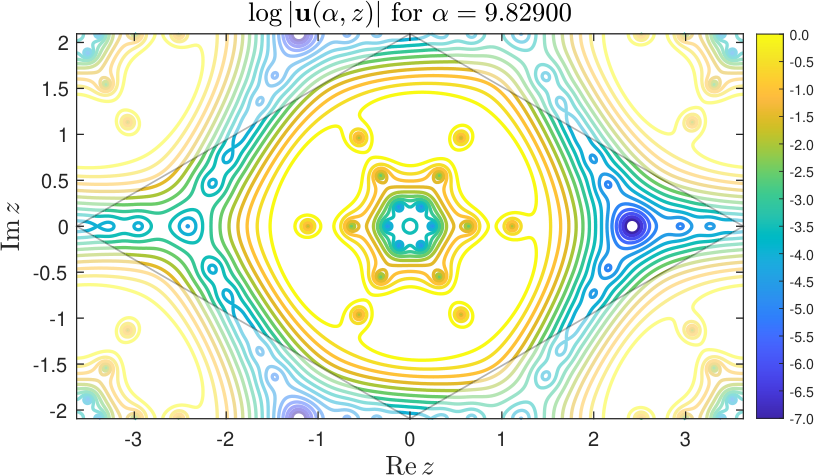
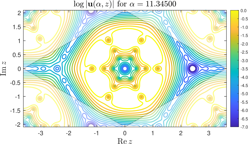
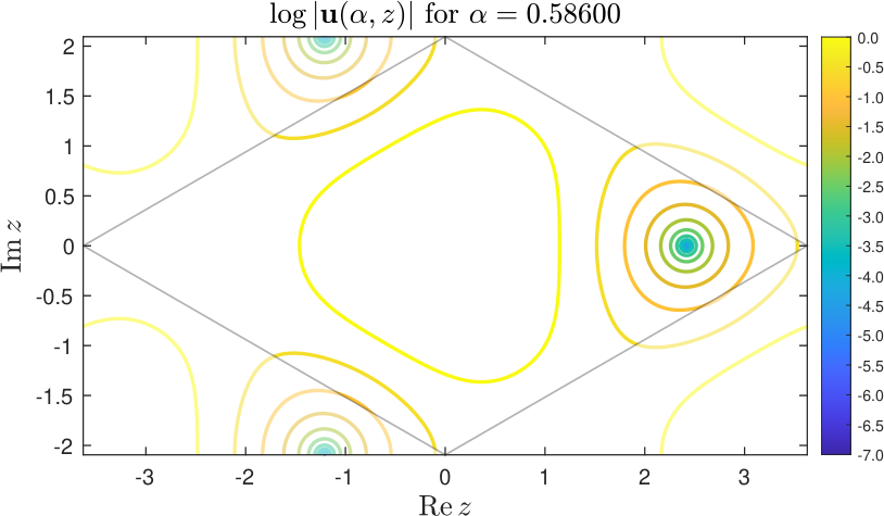
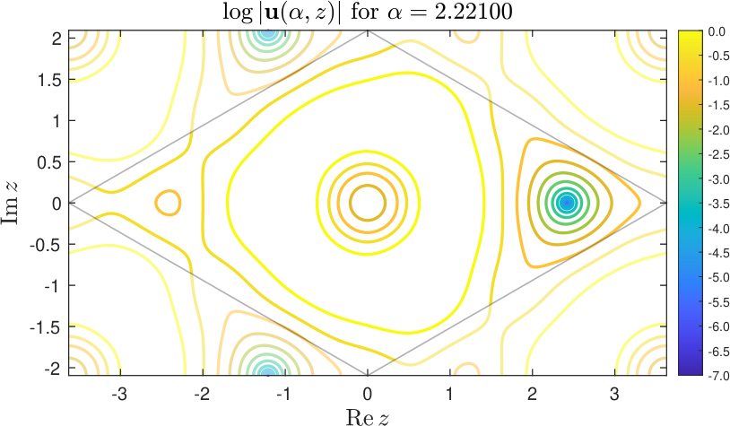
Figure 5. Plots of z↦log⁡|𝐮⁡(α,z)|z\mapsto\log|\mathbf{u}(\alpha,z)| (in the notation of Proposition 3.1) for α\alpha close to magic values (due to pseudospectral effects it is difficult to compute the exact eigenfunction at a magic angle) showing that the value of 𝐮\mathbf{u} at zS=4​39​πz_{S}=\frac{4\sqrt{3}}{9}\pi is close to 00.

3.2. A theta function argument

We first review basic definitions and properties of θ\theta functions – see [Mu83]. We have

θa,b(z|τ):=∑n∈ℤexp(πi(a+n)2τ+2πi(n+a)(z+b)),Imτ>0,θa,b(z+1|τ)=e2​π​i​aθa,b(z|τ),θa,b(z+τ|τ)=e−2​π​i​(z+b)−π​i​τθa,b(z|τ),θa+1,b(z|τ)=θa,b(z|τ),θa,b+1(z|τ)=e2​π​i​aθa,b(z|τ).\begin{gathered}\theta_{a,b}(z|\tau):=\sum_{n\in{\mathbb{Z}}}\exp(\pi i(a+n)^{2}\tau+2\pi i(n+a)(z+b)),\ \ \Imag\tau>0,\\ \theta_{a,b}(z+1|\tau)=e^{2\pi ia}\theta_{a,b}(z|\tau),\ \ \theta_{a,b}(z+\tau|\tau)=e^{-2\pi i(z+b)-\pi i\tau}\theta_{a,b}(z|\tau),\\ \theta_{a+1,b}(z|\tau)=\theta_{a,b}(z|\tau),\ \ \ \theta_{a,b+1}(z|\tau)=e^{2\pi ia}\theta_{a,b}(z|\tau).\end{gathered} (3.6)

The (simple) zeros of the (entire) function z↦θa,b​(z|τ)z\mapsto\theta_{a,b}(z|\tau) are given by

zn,m=(n−12−a)​τ+12−b−m.z_{n,m}=(n-\tfrac{1}{2}-a)\tau+\tfrac{1}{2}-b-m. (3.7)

If

g⁡(z):=θa′,b′​(z/τ′|τ)θa,b​(z/τ′|τ),g(z):=\frac{\theta_{a^{\prime},b^{\prime}}(z/\tau^{\prime}|\tau)}{\theta_{a,b}(z/\tau^{\prime}|\tau)}, (3.8)

then (3.6) shows that

g⁡(z+τ′)=e2​π​i​(a′−a)​g​(z),g⁡(z+τ​τ′)=e−2​π​i​(b′−b)​g​(z),g(z+\tau^{\prime})=e^{2\pi i(a^{\prime}-a)}g(z),\ \ g(z+\tau\tau^{\prime})=e^{-2\pi i(b^{\prime}-b)}g(z), (3.9)

and from (3.7) we know the zeros and poles of gg.

With this in place we can prove

Proposition 3.4.

In the notation of Propositions 3.1 and 3.3 we have

v⁡(α)=0,α∈ℝ⟹α∈𝒜.v(\alpha)=0,\ \ \alpha\in{\mathbb{R}}\ \Longrightarrow\ \alpha\in\mathcal{A}.

Proof. If 𝐮⁡(α)=(ψ1,ψ2)\mathbf{u}(\alpha)=(\psi_{1},\psi_{2}) then

v⁡(α)=ψ1​(z)​ψ1​(−z)+ψ2​(z)​ψ2​(−z).v(\alpha)=\psi_{1}(z)\psi_{1}(-z)+\psi_{2}(z)\psi_{2}(-z).

As remarked after (1.5), v⁡(α)v(\alpha) is independent of zz.

The observation made in [TKV19] is that ψ2\psi_{2} vanishes at special stacking points. These are fixed points of the action z↦ω​zz\mapsto\omega z on ℂ/Γ3{\mathbb{C}}/\Gamma_{3} (see (2.4)):

ψ2(α,±zS)=0,zS:=13(𝐚2−𝐚1)=4​39π,𝐚j=43πiωj.\begin{gathered}\psi_{2}(\alpha,\pm z_{S})=0,\ \ z_{S}:=\tfrac{1}{3}(\mathbf{a}_{2}-\mathbf{a}_{1})=\tfrac{4\sqrt{3}}{9}\pi,\ \ \mathbf{a}_{j}=\tfrac{4}{3}\pi i\omega^{j}.\end{gathered} (3.10)

To see this, note that (with the action of 𝒞\mathscr{C} identified with the action on (𝐮,0ℂ2)t∈L2​(ℂ/Γ,ℂ4)(\mathbf{u},0_{{\mathbb{C}}^{2}})^{t}\in L^{2}({\mathbb{C}}/\Gamma;{\mathbb{C}}^{4}))

𝐮⁡(α,±zS)=𝒞​𝐮​(α,±zS)=𝐮⁡(α,±ω​zS)=𝐮⁡(α,±zS∓𝐚2)=(ω±1001)​ℒ∓𝐚2​𝐮​(α,±zS)=(100ω∓1)​𝐮​(α,±zS).\begin{split}\mathbf{u}(\alpha,\pm z_{S})&=\mathscr{C}\mathbf{u}(\alpha,\pm z_{S})=\mathbf{u}(\alpha,\pm\omega z_{S})=\mathbf{u}(\alpha,\pm z_{S}\mp\mathbf{a}_{2})\\ &=\begin{pmatrix}\omega^{\pm 1}&0\\ 0&1\end{pmatrix}\mathscr{L}_{\mp\mathbf{a}_{2}}\mathbf{u}(\alpha,\pm z_{S})=\begin{pmatrix}1&0\\ 0&\omega^{\mp 1}\end{pmatrix}\mathbf{u}(\alpha,\pm z_{S}).\end{split}

Hence ψ2​(±zS)=ω∓1​ψ2​(±zS)\psi_{2}(\pm z_{S})=\omega^{\mp 1}\psi_{2}(\pm z_{S}), which proves (3.10).

We conclude that if v⁡(α)=0v(\alpha)=0 then ψ1​(zS)​ψ1​(−zS)=0\psi_{1}(z_{S})\psi_{1}(-z_{S})=0, and hence 𝐮⁡(α,zS)=0\mathbf{u}(\alpha,z_{S})=0 or 𝐮⁡(α,−zS)=0\mathbf{u}(\alpha,-z_{S})=0. Assume the former holds (otherwise we replace 𝐮\mathbf{u} with ℰ​𝐮\mathscr{E}\mathbf{u}). We can then construct a periodic solution to (D⁡(α)−𝐤)​𝐯𝐤=0(D(\alpha)-\mathbf{k})\mathbf{v}_{\mathbf{k}}=0 for any 𝐤∈ℂ\mathbf{k}\in{\mathbb{C}}, and in particular for 𝐤∉Γ∗\mathbf{k}\notin\Gamma^{*}, implying, in view of (3.3), that α∈𝒜\alpha\in\mathcal{A}.

In fact, if f𝐤f_{\mathbf{k}} is holomorphic with simple poles at the zeros of 𝐮\mathbf{u} allowed (we note that the equations 2​Dz¯​ψ1+U⁡(z)​ψ2=2​Dz¯​ψ2+U⁡(−z)​ψ1=02D_{\bar{z}}\psi_{1}+U(z)\psi_{2}=2D_{\bar{z}}\psi_{2}+U(-z)\psi_{1}=0 imply that ∂z¯ℓψj​(zS)=0\partial_{\bar{z}}^{\ell}\psi_{j}(z_{S})=0 and hence 𝐮=(z−zS)​𝐮~\mathbf{u}=(z-z_{S})\widetilde{\mathbf{u}}, where 𝐮~\widetilde{\mathbf{u}} is smooth near zSz_{S}) then

(D⁡(α)−𝐤)​𝐯𝐤=0,𝐯𝐤​(z)=ei2​(z​𝐤¯+z¯​𝐤)​f𝐤​(z)​𝐯​(z).(D(\alpha)-\mathbf{k})\mathbf{v}_{\mathbf{k}}=0,\ \ \ \mathbf{v}_{\mathbf{k}}(z)=e^{\frac{i}{2}(z\bar{\mathbf{k}}+\bar{z}{\mathbf{k}})}f_{\mathbf{k}}(z)\mathbf{v}(z).

To obtain periodicity we need

f𝐤(z+𝐚)=e−i2​(𝐚​𝐤¯+𝐚¯​𝐤)f𝐤(z),𝐚∈Γ,12(𝐚𝐤¯+𝐚¯𝐤)=2π(a1k1+a2k2),𝐚=4π(a1iω+a2iω2),𝐤=13(k1ω2−k2ω).\begin{gathered}f_{\mathbf{k}}(z+\mathbf{a})=e^{-\frac{i}{2}(\mathbf{a}\bar{\mathbf{k}}+\bar{\mathbf{a}}{\mathbf{k}})}f_{\mathbf{k}}(z),\ \ \mathbf{a}\in\Gamma,\ \ \tfrac{1}{2}(\mathbf{a}\bar{\mathbf{k}}+\bar{\mathbf{a}}{\mathbf{k}})=2\pi(a_{1}k_{1}+a_{2}k_{2}),\\ \mathbf{a}=4\pi(a_{1}i\omega+a_{2}i\omega^{2}),\ \ \mathbf{k}=\tfrac{1}{\sqrt{3}}(k_{1}\omega^{2}-k_{2}\omega).\end{gathered}

But now, (3.7)–(3.9) show that we can take

f𝐤​(z)=θ−16+k1/3,16−k2/3​(3​z/4​π​i​ω|ω)θ−16,16​(3​z/4​π​i​ω|ω).□\hskip 119.24506ptf_{\mathbf{k}}(z)=\frac{\theta_{-\frac{1}{6}+k_{1}/3,\frac{1}{6}-k_{2}/3}(3z/4\pi i\omega|\omega)}{\theta_{-\frac{1}{6},\frac{1}{6}}(3z/4\pi i\omega|\omega)}.\hskip 119.24506pt\Box
Proof of Theorem 2.

The lack of dependence of the spectrum of T𝐤T_{\mathbf{k}} on 𝐤∉Γ∗\mathbf{k}\notin\Gamma^{*} and equivalence of statements (1) and (2) are the content of Proposition 3.1. The definition of H𝐤​(α)H_{\mathbf{k}}(\alpha) in (1.4) immediately shows their equivalence to statement (3). ∎

Proof of Theorem 1.

In Proposition 3.1 we already obtained a (real) analytic family α↦𝐮⁡(α)\alpha\mapsto\mathbf{u}(\alpha). Then v⁡(α)=W⁡(𝐮⁡(α),ℰ​𝐮​(α))v(\alpha)=W(\mathbf{u}(\alpha),\mathscr{E}\mathbf{u}(\alpha)) and the equivalence of v⁡(α)v(\alpha) to (1) in Theorem 2 follows from Proposition 3.3 and 3.4. ∎

Remarks. 1. The zero of 𝐮⁡(α)∈kerLρ1,02​(ℂ/Γ,ℂ2)⁡D⁡(α)\mathbf{u}(\alpha)\in\ker_{L^{2}_{\rho_{1,0}}({\mathbb{C}}/\Gamma,{\mathbb{C}}^{2})}D(\alpha) seems to occur at zSz_{S} only – see Figure 5. This is also suggested by the following argument: from v⁡(α)=0v(\alpha)=0 we see that ℰ​𝐮​(z)=f⁡(z)​𝐮​(z)\mathscr{E}\mathbf{u}(z)=f(z)\mathbf{u}(z), where, using v⁡(α)=0v(\alpha)=0 again,

f⁡(z):=ψ2​(−z)ψ1​(z)=−ψ1​(−z)ψ2​(z)=α​U​(z)​ψ1​(−z)2​Dz¯​ψ​(z),f(z):=\frac{\psi_{2}(-z)}{\psi_{1}(z)}=-\frac{\psi_{1}(-z)}{\psi_{2}(z)}=\frac{\alpha U(z)\psi_{1}(-z)}{2D_{\bar{z}}\psi(z)}, (3.11)

is holomorphic away from ψ1−1​(0)∩(Dz¯​ψ1)−1​(0)\psi_{1}^{-1}(0)\cap(D_{\bar{z}}\psi_{1})^{-1}(0). We also see that ff is meromorphic: in fact, near any point z0z_{0}, ψ1​(z0+ζ)=F1​(ζ,ζ¯)\psi_{1}(z_{0}+\zeta)=F_{1}(\zeta,\bar{\zeta}), ψ2​(−z0−ζ)=F2​(ζ,ζ¯)\psi_{2}(-z_{0}-\zeta)=F_{2}(\zeta,\bar{\zeta}), where Fj:Bℂ2​(0,δ)→ℂF_{j}:B_{{\mathbb{C}}^{2}}(0,\delta)\to{\mathbb{C}} are holomorphic functions (this follows from real analyticity of ψj\psi_{j}, which follows in turn from the ellipticity of the equation – see [HöI, Theorem 8.6.1]). The definition of ff and the fact that ∂z¯f=0\partial_{\bar{z}}f=0 away from zeros of ψ1\psi_{1} shows that F2​(ζ,ξ)=f⁡(z0+ζ)​F1​(ζ,ξ)F_{2}(\zeta,\xi)=f(z_{0}+\zeta)F_{1}(\zeta,\xi). We can then choose ξ0\xi_{0} such that F1​(ζ,ξ0)F_{1}(\zeta,\xi_{0}) is not identically zero (if no such ξ0\xi_{0} existed, ψ1≡0\psi_{1}\equiv 0, and hence, from the equation, 𝐮≡0\mathbf{u}\equiv 0). But then ζ↦f⁡(z0+ζ)=F2​(ζ,ξ0)/F1​(ζ,ξ0)\zeta\mapsto f(z_{0}+\zeta)=F_{2}(\zeta,\xi_{0})/F_{1}(\zeta,\xi_{0}) is meromorphic near ζ=0\zeta=0 and, as z0z_{0} was arbitrary, everywhere. In addition,

f⁡(z+𝐚)=ω−a1−a2​f​(z),𝐚∈Γ3,f⁡(ω​z)=f⁡(z),f⁡(z)​f​(−z)=−1.f(z+\mathbf{a})=\omega^{-a_{1}-a_{2}}f(z),\ \ \mathbf{a}\in\Gamma_{3},\ \ f(\omega z)=f(z),\ \ f(z)f(-z)=-1.

These symmetries also show that f⁡(zS+ω​ζ)=ω−1​f​(zS+ζ)f(z_{S}+\omega\zeta)=\omega^{-1}f(z_{S}+\zeta), which means that f⁡(zS+ζ)=∑k≥k0ζ−1+3​k​fkf(z_{S}+\zeta)=\sum_{k\geq k_{0}}\zeta^{-1+3k}f_{k} and f⁡(−zS−ζ)=∑ℓ≥1−k0ζ−2+3​ℓ​gℓf(-z_{S}-\zeta)=\sum_{\ell\geq 1-k_{0}}\zeta^{-2+3\ell}g_{\ell}, for some k0∈ℤk_{0}\in{\mathbb{Z}}. Hence, if ff has only poles of order 1, we have 𝐮⁡(α,zS)=0\mathbf{u}(\alpha,z_{S})=0. We formulate this bold guess as follows:

𝐮⁡(α)∈kerLρ1,02​(ℂ/Γ,ℂ2)⁡D⁡(α),𝐮⁡(α)≢0⟹𝐮⁡(α,z)≠0,z∉zS+Γ3.\mathbf{u}(\alpha)\in\ker_{L^{2}_{\rho_{1,0}}({\mathbb{C}}/\Gamma,{\mathbb{C}}^{2})}D(\alpha),\ \ \mathbf{u}(\alpha)\not\equiv 0\ \Longrightarrow\ \mathbf{u}(\alpha,z)\neq 0,\ \ z\notin z_{S}+\Gamma_{3}. (3.12)

This is related to the following fact, which seems to hold as well:

dimkerLρ1,02​(ℂ/Γ,ℂ2)⁡D⁡(α)=1,α∈ℂ.\dim\ker_{L^{2}_{\rho_{1,0}}({\mathbb{C}}/\Gamma,{\mathbb{C}}^{2})}D(\alpha)=1,\ \ \alpha\in{\mathbb{C}}. (3.13)
Proof of (3.12) ⇒\Rightarrow (3.13).

Suppose that 𝐮=(ψ1,ψ2)t\mathbf{u}=(\psi_{1},\psi_{2})^{t} and 𝐯=(φ1,φ2)t\mathbf{v}=(\varphi_{1},\varphi_{2})^{t} are two elements of the kernel in Lρ1,02L^{2}_{\rho_{1,0}}. We then define the (constant) Wronskian w:=ψ1​φ2−ψ2​φ1w:=\psi_{1}\varphi_{2}-\psi_{2}\varphi_{1}. Since φ2​(±zS)=ψ2​(±zS)=0\varphi_{2}(\pm z_{S})=\psi_{2}(\pm z_{S})=0 (see (3.10)), we have w=0w=0 and hence 𝐯=g​𝐮\mathbf{v}=g\mathbf{u}, where g⁡(z)=φ1​(z)/ψ1​(z)g(z)=\varphi_{1}(z)/\psi_{1}(z). As in the discussion of ff given after (3.11), we see that g⁡(z)g(z) is a meromorphic function periodic with respect to Γ3\Gamma_{3}. From (3.12) applied to ψ1\psi_{1} we see that gg can only have poles at zS+Γ3z_{S}+\Gamma_{3}, and applied to φ1​(z)\varphi_{1}(z) we see that gg can only have zeros at the same place. But this implies that gg is constant. ∎

2. The elements of the kernel of D⁡(α)−𝐤D(\alpha)-\mathbf{k} can be obtained from the (finite rank) residue of the operator (3.5), and theta functions are already implicitly present there. On one hand (see §5) the operator (2​Dz¯−𝐤)−1(2D_{\bar{z}}-\mathbf{k})^{-1} can be described using Fourier expansion, but on the other hand it can be represented using theta functions: it is the convolution with the fundamental solution of 2​Dz¯−𝐤2D_{\bar{z}}-\mathbf{k} on ℂ/Γ{\mathbb{C}}/\Gamma. To obtain the convolution kernel (in a construction which works for any torus) we seek a function G𝐤G_{\mathbf{k}} such that

(2Dz¯−𝐤)G𝐤=δ0(z),G𝐤=ei2​(𝐤​z¯+𝐤¯​z)g𝐤(z),∂z¯g𝐤|ℂ∖Γ=0,g𝐤​(z+𝐚)=e−i2​(𝐤¯​𝐚+𝐤​𝐚¯)​g𝐤​(z),Resz=w​g𝐤​(z)={i/(2​π),w∈Γ; 0,w∉Γ.\begin{gathered}(2D_{\bar{z}}-\mathbf{k})G_{\mathbf{k}}=\delta_{0}(z),\ \ \ G_{\mathbf{k}}=e^{\frac{i}{2}(\mathbf{k}\bar{z}+\bar{\mathbf{k}}z)}g_{\mathbf{k}}(z),\ \ \ \partial_{\bar{z}}g_{\mathbf{k}}|_{{\mathbb{C}}\setminus\Gamma}=0,\\ g_{\mathbf{k}}(z+\mathbf{a})=e^{-\frac{i}{2}(\bar{\mathbf{k}}\mathbf{a}+\mathbf{k}\bar{\mathbf{a}})}g_{\mathbf{k}}(z),\ \ \ {\rm{Res}}_{z=w}g_{\mathbf{k}}(z)=\left\{\begin{array}[]{ll}i/(2\pi),&w\in\Gamma;\\ \ \ 0,&w\notin\Gamma.\end{array}\right.\end{gathered}

(The last condition gives 2​Dz¯​g𝐤​(z)=∑𝐚∈Γδ𝐚​(z)2D_{\bar{z}}g_{\mathbf{k}}(z)=\sum_{\mathbf{a}\in\Gamma}\delta_{\mathbf{a}}(z), as ∂z¯(1/(π​z))=δ0​(z)\partial_{\bar{z}}(1/(\pi z))=\delta_{0}(z).)

To find g𝐤g_{\mathbf{k}} we return to (3.7) and (3.8) and choose

τ′=4​π​i​ω,τ​τ′=4​π​i​ω2,a=12,b=12,a′=12−k1,b′=12+k2.\tau^{\prime}=4\pi i\omega,\ \ \tau\tau^{\prime}=4\pi i\omega^{2},\ \ a=\tfrac{1}{2},\ \ b=\tfrac{1}{2},\ \ a^{\prime}=\tfrac{1}{2}-k_{1},\ \ b^{\prime}=\tfrac{1}{2}+k_{2}.

Hence we have

g𝐤​(z):=e−π​i​k12+2​π​i​k1​(12+k2)​θ12,12′​(0|ω)OPEN2​π​i​θ12,12​(ω​k1+k2)|ω)​θ12−k1,12+k2​(z/4​π​i​ω|ω)θ12,12​(z/4​π​i​ω|ω),𝐤=13(k1ω−k2ω2),(k1,k2)∉ℤ2.\begin{gathered}g_{\mathbf{k}}(z):=\frac{e^{-\pi ik_{1}^{2}+2\pi ik_{1}(\frac{1}{2}+k_{2})}\theta_{\frac{1}{2},\frac{1}{2}}^{\prime}(0|\omega)}{2\pi i\theta_{\frac{1}{2},\frac{1}{2}}(\omega k_{1}+k_{2})|\omega)}\frac{\theta_{\frac{1}{2}-k_{1},\frac{1}{2}+k_{2}}(z/4\pi i\omega|\omega)}{\theta_{\frac{1}{2},\frac{1}{2}}(z/4\pi i\omega|\omega)},\\ \mathbf{k}=\tfrac{1}{\sqrt{3}}(k_{1}\omega-k_{2}\omega^{2}),\ \ (k_{1},k_{2})\notin{\mathbb{Z}}^{2}.\end{gathered} (3.14)

It would be interesting to derive (1.8) from (3.5) and (3.14). ∎

3.3. Existence of magic α\alpha’s

We now give a proof of Theorem 3 which amounts to calculating tr⁡T𝐤4\tr T_{\mathbf{k}}^{4}. For that it is convenient to switch to rectangular coordinates, which are also used in numerical computations (see §5): z=x1+i​x2=2​i​ω​y1+2​i​ω2​y2z=x_{1}+ix_{2}=2i\omega y_{1}+2i\omega^{2}y_{2}. We have U⁡(z)=e−i⁡(y1+y2)+ω​ei⁡(2​y1−y2)+ω2​ei⁡(−y1+2​y2)U(z)=e^{-i(y_{1}+y_{2})}+\omega e^{i(2y_{1}-y_{2})}+\omega^{2}e^{i(-y_{1}+2y_{2})} and 2​Dz¯=Dx1+i​Dx2=(ω2​Dy1−ω​Dy2)/32D_{\bar{z}}=D_{x_{1}}+iD_{x_{2}}=\left(\omega^{2}D_{y_{1}}-\omega D_{y_{2}}\right)/\sqrt{3}. We are then studying

D𝐤​(α):=D⁡(α)+𝐤=13​(𝒟𝐤α​𝒱​(y)α​𝒱​(−y)𝒟𝐤),𝒟𝐤:=ω2​(Dy1+k1)−ω⁡(Dy2+k2),𝒱⁡(y):=3​(e−i⁡(y1+y2)+ω​ei⁡(2​y1−y2)+ω2​ei⁡(−y1+2​y2)),\begin{gathered}D_{\mathbf{k}}(\alpha):=D(\alpha)+\mathbf{k}=\tfrac{1}{\sqrt{3}}\begin{pmatrix}\mathscr{D}_{\mathbf{k}}&\alpha\mathscr{V}(y)\\ \alpha\mathscr{V}(-y)&\mathscr{D}_{\mathbf{k}}\end{pmatrix},\\ \mathscr{D}_{\mathbf{k}}:={\omega^{2}(D_{y_{1}}+k_{1})-\omega(D_{y_{2}}+k_{2})},\\ \mathscr{V}(y):=\sqrt{3}(e^{-i(y_{1}+y_{2})}+\omega e^{i(2y_{1}-y_{2})}+\omega^{2}e^{i(-y_{1}+2y_{2})}),\end{gathered} (3.15)

with periodic periodic boundary conditions (for y↦y+2​π​𝐧y\mapsto y+2\pi\mathbf{n}, 𝐧∈ℤ2\mathbf{n}\in{\mathbb{Z}}^{2}). In the following, we shall write 𝒱±​(y):=𝒱⁡(±y).\mathscr{V}_{\pm}(y):=\mathscr{V}(\pm y). The operator T𝐤T_{\mathbf{k}}, 𝐤=(ω2​k1−ω​k2)/3\mathbf{k}=(\omega^{2}k_{1}-\omega k_{2})/\sqrt{3}, (k1,k2)∉ℤ2(k_{1},k_{2})\notin{\mathbb{Z}}^{2}, is given by

T𝐤:=(0𝒟𝐤−1​𝒱+𝒟𝐤−1​𝒱−0).T_{\mathbf{k}}:=\begin{pmatrix}0&\mathscr{D}_{\mathbf{k}}^{-1}\mathscr{V}_{+}\\ \mathscr{D}_{\mathbf{k}}^{-1}\mathscr{V}_{-}&0\end{pmatrix}.

In this notation,

tr⁡T𝐤4=18​tr⁡A2,A:=A𝐤:=13​𝒟𝐤−1​𝒱+​𝒟𝐤−1​𝒱−,\tr T_{\mathbf{k}}^{4}=18\tr A^{2},\ \ A:=A_{\mathbf{k}}:=\tfrac{1}{3}\mathscr{D}_{\mathbf{k}}^{-1}\mathscr{V}_{+}\mathscr{D}_{\mathbf{k}}^{-1}\mathscr{V}_{-}, (3.16)

where we note that A2A^{2}, a pseudodifferential operator of order −4-4, is of trace class (see for instance [DyZw19, Theorem B.21]).

By taking the (discrete) Fourier transform on ℝ2/2​π​ℤ2{\mathbb{R}}^{2}/2\pi{\mathbb{Z}}^{2} we consider the operator D𝐤​(α)D_{\mathbf{k}}(\alpha) as acting on ℓ2​(ℤ)⊗ℓ2​(ℤ)\ell^{2}({\mathbb{Z}})\otimes\ell^{2}({\mathbb{Z}}). With D:=diag​(ℓ)ℓ∈ℤD:={\rm{diag}}\,(\ell)_{\ell\in{\mathbb{Z}}} and OPENJ⁡((an)n∈ℤ))=(an+1)n∈ℤJ((a_{n})_{n\in{\mathbb{Z}}}))=(a_{n+1})_{n\in{\mathbb{Z}}}, we have

𝒟𝐤=ω2​(D+k1)⊗I−ω​I⊗(D+k2​I),𝒱+/3=J⊗J+ω​J−2⊗J+ω2​J⊗J−2,𝒱−/3=J−1⊗J−1+ω​J2⊗J−1+ω2​J−1⊗J2.\begin{split}\mathscr{D}_{\mathbf{k}}&=\omega^{2}(D+k_{1})\otimes I-\omega I\otimes(D+k_{2}I),\\ \mathscr{V}_{+}/\sqrt{3}&=J\otimes J+\omega\,J^{-2}\otimes J+\omega^{2}J\otimes J^{-2},\\ \mathscr{V}_{-}/\sqrt{3}&=J^{-1}\otimes J^{-1}+\omega J^{2}\otimes J^{-1}+\omega^{2}\,J^{-1}\otimes J^{2}.\end{split} (3.17)

The numerical value in Theorem 3 will come from the following, surely classical, computation:

Lemma 3.5.

For Γ:=ω​ℤ⊕ℤ\Gamma:=\omega{\mathbb{Z}}\oplus{\mathbb{Z}}, ω:=e2​π​i/3\omega:=e^{2\pi i/3} and γ0∈Γ∖{0}\gamma_{0}\in\Gamma\setminus\{0\} define

K⁡(γ0):=∑γ∈Γ∖{0,γ0}γ−2​(γ−γ0)−2.K(\gamma_{0}):=\sum_{\gamma\in\Gamma\setminus\{0,\gamma_{0}\}}\gamma^{-2}(\gamma-\gamma_{0})^{-2}. (3.18)

Then

K⁡(ω​m+n)=−4​π​i​(ω⁡(2​n−m)+n+m)3​(ω​m+n)3.K(\omega m+n)=-\frac{4\pi i(\omega(2n-m)+n+m)}{3(\omega m+n)^{3}}. (3.19)
Proof.

We notice that K⁡(ω​γ0)=ω¯​K​(γ0)K(\omega\gamma_{0})=\bar{\omega}K(\gamma_{0}). Hence it is enough to evaluate

g⁡(γ0):=∑j=02ωj​K​(ωj​γ0)=3​K​(γ0).g(\gamma_{0}):=\sum_{j=0}^{2}\omega^{j}K(\omega^{j}\gamma_{0})=3K(\gamma_{0}). (3.20)

Also, if we define F⁡(z,γ0):=∑γ∈Γ(γ−z)−2​(γ−γ0−z)−2F(z,\gamma_{0}):=\sum_{\gamma\in\Gamma}(\gamma-z)^{-2}(\gamma-\gamma_{0}-z)^{-2}, then FF is a meromorphic Γ\Gamma-periodic function with the singularity at z=0z=0 given by 2/(z​γ0)22/(z\gamma_{0})^{2}. Hence,

F⁡(z,γ0)=2​γ0−2​℘​(z)+K⁡(γ0),℘⁡(z):=∑γ∈Γ(1(γ−z)2−1−δγ,0γ2).F(z,\gamma_{0})=2\gamma_{0}^{-2}\wp(z)+K(\gamma_{0}),\ \ \ \wp(z):=\sum_{\gamma\in\Gamma}\left(\frac{1}{(\gamma-z)^{2}}-\frac{1-\delta_{\gamma,0}}{\gamma^{2}}\right).

Using the partial fraction expansion, the fact that ∑j=02ωj=0\sum_{j=0}^{2}\omega^{j}=0 and the above series for the ℘\wp-function, we obtain

g⁡(γ0)=∑j=02ωj​F​(z,ωj​γ0)=γ0−2​∑γ∈Γ∑j=02ω¯j​(1(γ−ωj​γ0−z)2−2​ω¯jγ0​1(γ−ωj​γ0−z))=γ0−2​∑j=02ω¯j​℘​(z)+∑γ∈Γ∑j=02ω¯jγ02​1−δγ,ωj​γ0(γ−ωj​γ0)2−∑γ∈Γ∑j=022​ωjγ03​1(γ−ωj​γ0−z),\begin{split}g(\gamma_{0})&=\sum_{j=0}^{2}\omega^{j}F(z,\omega^{j}\gamma_{0})=\gamma_{0}^{-2}\sum_{\gamma\in\Gamma}\sum_{j=0}^{2}\bar{\omega}^{j}\left(\frac{1}{(\gamma-\omega^{j}\gamma_{0}-z)^{2}}-\frac{2\bar{\omega}^{j}}{\gamma_{0}}\frac{1}{(\gamma-\omega^{j}\gamma_{0}-z)}\right)\\ &=\gamma_{0}^{-2}\sum_{j=0}^{2}\bar{\omega}^{j}\wp(z)+\sum_{\gamma\in\Gamma}\sum_{j=0}^{2}\frac{\bar{\omega}^{j}}{\gamma_{0}^{2}}\frac{1-\delta_{\gamma,\omega^{j}\gamma_{0}}}{(\gamma-\omega^{j}\gamma_{0})^{2}}-\sum_{\gamma\in\Gamma}\sum_{j=0}^{2}\frac{2\omega^{j}}{\gamma_{0}^{3}}\frac{1}{(\gamma-\omega^{j}\gamma_{0}-z)},\end{split}

where the first term on the right hand side vanishes and both series converge absolutely (this can be checked by taking a common denominator using ∏j=02(ζ−ωj​γ0)=ζ3−γ02\prod_{j=0}^{2}(\zeta-\omega^{j}\gamma_{0})=\zeta^{3}-\gamma_{0}^{2}). We now have

∑γ∈Γ∑j=02ω¯j​1−δγ,ωj​γ0(γ−ωj​γ0)2=limN→∞∑j=02ω¯j​∑|γ−ωj​γ0|≤N(1−δγ,0)​γ−2=𝒪⁡(1)​limN→∞∑N−|γ0|≤|γ|≤N+|γ0|N−2=0.\begin{split}\sum_{\gamma\in\Gamma}\sum_{j=0}^{2}{\bar{\omega}^{j}}\frac{1-\delta_{\gamma,\omega^{j}\gamma_{0}}}{(\gamma-\omega^{j}\gamma_{0})^{2}}&=\lim_{N\to\infty}\sum_{j=0}^{2}\bar{\omega}^{j}\sum_{|\gamma-\omega^{j}\gamma_{0}|\leq N}(1-\delta_{\gamma,0}){\gamma^{-2}}\\ &=\mathcal{O}(1)\lim_{N\to\infty}\sum_{N-|\gamma_{0}|\leq|\gamma|\leq N+|\gamma_{0}|}N^{-2}=0.\end{split}

Hence, using the fact that ∑n∈ℤ((n−a)−1−(n−b)−1)=π​cot⁡π​b−π​cot⁡π​a\sum_{n\in{\mathbb{Z}}}((n-a)^{-1}-(n-b)^{-1})=\pi\cot\pi b-\pi\cot\pi a,

g⁡(γ0)=2​π​γ0−3​limM→∞∑m=−MM∑j=02ωj​(cot⁡π⁡(m​ω+ωj​γ0+z)−cot⁡π⁡(m​ω+z)).\begin{split}g(\gamma_{0})&=2\pi\gamma_{0}^{-3}\lim_{M\to\infty}\sum_{m=-M}^{M}\sum_{j=0}^{2}\omega^{j}\left(\cot\pi(m\omega+\omega^{j}\gamma_{0}+z)-\cot\pi(m\omega+z)\right).\end{split} (3.21)

Since cot⁡π​x−cot⁡π​y=2​i​((e2​π​i​x−1)−1−(e2​π​i​y−1)−1)\cot\pi x-\cot\pi y=2i((e^{2\pi ix}-1)^{-1}-(e^{2\pi iy}-1)^{-1}), e2​π​i​n​ω=(−1)n​e−n​π​3e^{2\pi in\omega}=(-1)^{n}e^{-n\pi\sqrt{3}}, n∈ℤn\in{\mathbb{Z}}, we obtain, with am:=(e2​π​i​(m​ω+z)−1)−1a_{m}:=(e^{2\pi i(m\omega+z)}-1)^{-1},

∑m=−MM(cot⁡((m+m0)​ω+n0−z)−cot⁡π⁡(m​ω−z))=2​i​∑m=−MM(am+m0−am)=2​i​∑m=M+1M+m0am−2​i​∑m=−M−M+m0+1am=2​i​∑m=M+1M+m0(−1+𝒪⁡(e−M))−2​i​∑m=M−m0+1M𝒪⁡(e−M)=−2​i​m0+𝒪⁡(e−M).\begin{split}&\sum_{m=-M}^{M}(\cot((m+m_{0})\omega+n_{0}-z)-\cot\pi(m\omega-z))\\ \ &\ \ \ \ \ \ =2i\sum_{m=-M}^{M}(a_{m+m_{0}}-a_{m})=2i\sum_{m=M+1}^{M+m_{0}}a_{m}-2i\sum_{m=-M}^{-M+m_{0}+1}a_{m}\\ &\ \ \ \ \ \ =2i\sum_{m=M+1}^{M+m_{0}}(-1+\mathcal{O}(e^{-M}))-2i\sum_{m=M-m_{0}+1}^{M}\mathcal{O}(e^{-M})=-2im_{0}+\mathcal{O}(e^{-M}).\end{split}

Inserting this in (3.21) with γ=ω​m0+n0\gamma=\omega m_{0}+n_{0} (and calculating the corresponding ωj​γ\omega^{j}\gamma) gives

g⁡(ω​m0+n0)=−4​π​i​(ω​m0+n0)−3​(ω⁡(2​n0−m0)+n0+m0),\begin{split}g(\omega m_{0}+n_{0})&=-4\pi i(\omega m_{0}+n_{0})^{-3}(\omega(2n_{0}-m_{0})+n_{0}+m_{0}),\end{split}

which, in view of (3.20), proves (3.19). ∎

We can now give the

Proof of Theorem 3.

To simplify calculations we introduce the following notation:

Jp,q:=Jp⊗Jq,p,q∈ℤ.J^{p,q}:=J^{p}\otimes J^{q},\ \ p,q\in{\mathbb{Z}}. (3.22)

Also, for a diagonal matrix Λ=(Λi​j)i,j∈ℤ\Lambda=(\Lambda_{ij})_{i,j\in{\mathbb{Z}}} acting on ℓ2​(ℤ)⊗ℓ2​(ℤ)\ell^{2}({\mathbb{Z}})\otimes\ell^{2}({\mathbb{Z}}) we define a new diagonal matrix with the following basic properties:

Λp,q:=(Λi+p,j+q)i,j∈ℤ,(ΛΛ′)p,q=Λp,qΛ′p,q,(Λp′,q′)p,q=Λp+p′,q+q′,\begin{gathered}\Lambda_{p,q}:=(\Lambda_{i+p,j+q})_{i,j\in{\mathbb{Z}}},\\ (\Lambda\Lambda^{\prime})_{p,q}=\Lambda_{p,q}\Lambda^{\prime}_{p,q},\ \ \ \ (\Lambda_{p^{\prime},q^{\prime}})_{p,q}=\Lambda_{p+p^{\prime},q+q^{\prime}},\end{gathered} (3.23)

where Λ′\Lambda^{\prime} is just another diagonal matrix. To express powers of AA in (3.16) we will use the following simple fact:

Jp,q​Λ​Jp′,q′=Λp,q​Jp+p′,q+q′=Jp+p′,q+q′​Λ−p′,−q′.J^{p,q}\Lambda J^{p^{\prime},q^{\prime}}=\Lambda_{p,q}J^{p+p^{\prime},q+q^{\prime}}=J^{p+p^{\prime},q+q^{\prime}}\Lambda_{-p^{\prime},-q^{\prime}}. (3.24)

If we put

Λ:=D𝐤−1,Λm​n=(ω2​(m+k1)−ω⁡(n+k2))−1,(k1,k2)∉ℤ2,\Lambda:=D_{\mathbf{k}}^{-1},\ \ \Lambda_{mn}=(\omega^{2}(m+k_{1})-\omega(n+k_{2}))^{-1},\ \ (k_{1},k_{2})\notin{\mathbb{Z}}^{2},

then, in the notation of (3.16),

A=Λ⁡(J1,1+ω​J−2,1+ω2​J1,−2)​Λ​(J−1,−1+ω​J2,−1+ω2​J−1,2)=Λ​Λ1,1+ω​Λ​Λ1,−2+ω2​Λ​Λ−2,1+ω​Λ​Λ1,1​J3,0+ω2​Λ​Λ1,1​J0,3+ω​Λ​Λ−2,1​J−3,0+ω2​Λ​Λ1,−2​J0,−3+Λ​Λ−2,1​J−3,3+Λ​Λ1,−2​J3,−3.\begin{split}A&=\Lambda(J^{1,1}+\omega J^{-2,1}+\omega^{2}J^{1,-2})\Lambda(J^{-1,-1}+\omega J^{2,-1}+\omega^{2}J^{-1,2})\\ &=\Lambda\Lambda_{1,1}+\omega\Lambda\Lambda_{1,-2}+\omega^{2}\Lambda\Lambda_{-2,1}+\omega\Lambda\Lambda_{1,1}J^{3,0}+\omega^{2}\Lambda\Lambda_{1,1}J^{0,3}\\ &\ \ \ +\omega\Lambda\Lambda_{-2,1}J^{-3,0}+\omega^{2}\Lambda\Lambda_{1,-2}J^{0,-3}+\Lambda\Lambda_{-2,1}J^{-3,3}+\Lambda\Lambda_{1,-2}J^{3,-3}.\end{split}

The diagonal part of A2A^{2} is then given by (note that the matrices are diagonal and commute)

B:=Λ2​Λ1,12+ω2​Λ2​Λ1,−22+ω​Λ2​Λ−2,12+2​ω​Λ2​Λ1,1​Λ1,−2+2​ω2​Λ2​Λ1,1​Λ−2,1+2​Λ2​Λ−2,1​Λ1,−2+ω2​Λ1,12​Λ​Λ3,0+ω2​Λ−2,12​Λ​Λ−3,0+ω​Λ1,12​Λ​Λ0,3+ω​Λ1,−22​Λ​Λ0,−3+Λ−2,12​Λ​Λ−3,3+Λ1,−22​Λ​Λ3,−3.\begin{split}B&:=\Lambda^{2}\Lambda_{1,1}^{2}+\omega^{2}\Lambda^{2}\Lambda_{1,-2}^{2}+\omega\Lambda^{2}\Lambda_{-2,1}^{2}+2\omega\Lambda^{2}\Lambda_{1,1}\Lambda_{1,-2}+2\omega^{2}\Lambda^{2}\Lambda_{1,1}\Lambda_{-2,1}\\ &\ \ \ +2\Lambda^{2}\Lambda_{-2,1}\Lambda_{1,-2}+\omega^{2}\Lambda_{1,1}^{2}\Lambda\Lambda_{3,0}+\omega^{2}\Lambda_{-2,1}^{2}\Lambda\Lambda_{-3,0}+\omega\Lambda_{1,1}^{2}\Lambda\Lambda_{0,3}\\ &\ \ \ +\omega\Lambda_{1,-2}^{2}\Lambda\Lambda_{0,-3}+\Lambda_{-2,1}^{2}\Lambda\Lambda_{-3,3}+\Lambda_{1,-2}^{2}\Lambda\Lambda_{3,-3}.\end{split} (3.25)

Since tr⁡Λk,ℓ2​Λp,q​Λp′,q′=tr⁡Λk+r,ℓ+s2​Λp+r,q+s​Λp′+r,q′+s\tr\Lambda^{2}_{k,\ell}\Lambda_{p,q}\Lambda_{p^{\prime},q^{\prime}}=\tr\Lambda^{2}_{k+r,\ell+s}\Lambda_{p{+}r,q{+}s}\Lambda_{p^{\prime}{+}r,q^{\prime}{+}s}, we have

tr⁡A2=tr⁡Λ2​(Λ1,12+2​Λ−2,1​Λ1,−2+2​Λ2,−1​Λ−1,2)+ω​tr⁡Λ2​(Λ−2,12+2​Λ1,1​Λ1,−2+2​Λ−1,2​Λ−1,−1)+ω2​tr⁡Λ2​(Λ1,−22+2​Λ1,1​Λ−2,1+2​Λ−1,−1​Λ2,−1).\begin{split}\tr A^{2}&=\tr\Lambda^{2}(\Lambda_{1,1}^{2}+2\Lambda_{-2,1}\Lambda_{1,-2}+2\Lambda_{2,-1}\Lambda_{-1,2})\\ &\ \ \ +\omega\tr\Lambda^{2}(\Lambda_{-2,1}^{2}+2\Lambda_{1,1}\Lambda_{1,-2}+2\Lambda_{-1,2}\Lambda_{-1,-1})\\ &\ \ \ +\omega^{2}\tr\Lambda^{2}(\Lambda_{1,-2}^{2}+2\Lambda_{1,1}\Lambda_{-2,1}+2\Lambda_{-1,-1}\Lambda_{2,-1}).\end{split}

We now find that

Λ±2,∓1​Λ∓1,±2+ω​Λ∓1,±2​Λ∓1,∓1+ω2​Λ∓1,∓1​Λ±2,±1=0.\Lambda_{\pm 2,\mp 1}\Lambda_{\mp 1,\pm 2}+\omega\Lambda_{\mp 1,\pm 2}\Lambda_{\mp 1,\mp 1}+\omega^{2}\Lambda_{\mp 1,\mp 1}\Lambda_{\pm 2,\pm 1}=0.

In fact, using

1a​b+1b​c+1c​a=a+b+ca​b​c\frac{1}{ab}+\frac{1}{bc}+\frac{1}{ca}=\frac{a+b+c}{abc}

it suffices to show, say for the ++ case, that for all n∈ℤ2n\in{\mathbb{Z}}^{2}

ω​(Λ2,−1)n,n−1+ω¯​(Λ−1,2)n,n−1+(Λ−1,−1)n,n−1=0\omega(\Lambda_{2,-1})_{n,n}^{-1}+\bar{\omega}(\Lambda_{-1,2})_{n,n}^{-1}+(\Lambda_{-1,-1})_{n,n}^{-1}=0

which follows from a direct computation. Hence, the expression for the trace simplifies further to

tr⁡A2=tr⁡Λ2​(Λ1,12+ω​Λ−2,12+ω2​Λ1,−22),\begin{split}\tr A^{2}=\tr\Lambda^{2}(\Lambda_{1,1}^{2}+\omega\Lambda_{-2,1}^{2}+\omega^{2}\Lambda_{1,-2}^{2}),\end{split} (3.26)

and this expression can be calculated using Lemma 3.5. The singular terms of the sum in (3.26) cancel, as the proof of Lemma 3.5 shows, so we can remove them, and put k1=k2=0k_{1}=k_{2}=0. Noting that ω2​m−ω​n=ω​γ\omega^{2}m-\omega n=\omega\gamma, γ=ω​m−n\gamma=\omega m-n, and ω2​(m+p)−ω⁡(n+q)=ω⁡(γ−γ0)\omega^{2}(m+p)-\omega(n+q)=\omega(\gamma-\gamma_{0}), γ0=−ω​p+q\gamma_{0}=-\omega p+q,

tr⁡A2=ω¯​K​(−ω+1)+K⁡(2​ω+1)+ω​K​(−ω−2)=K⁡(2​ω+1)+ω​K​(ω⁡(2​ω+1))+ω2​K​(ω2​(2​ω+1))=3​K​(2​ω+1)=4​π/3,\begin{split}\tr A^{2}&=\bar{\omega}K(-\omega+1)+K(2\omega+1)+\omega K(-\omega-2)\\ &=K(2\omega+1)+\omega K(\omega(2\omega+1))+\omega^{2}K(\omega^{2}(2\omega+1))=3K(2\omega+1)\\ &={4\pi}/\sqrt{3},\end{split}

where we used (3.19) and (3.20). In view of (3.16), this concludes the proof. ∎

Remark. Similar arguments can be used to show that ∑α∈𝒜α−8=tr⁡T𝐤4=740​π/3\sum_{\alpha\in\mathcal{A}}\alpha^{-8}=\tr T_{\mathbf{k}}^{4}=740\pi/\sqrt{3}.

4. Exponential squeezing of bands

Here we prove a more general version of Theorem 4 valid for potentials with symmetries (2.1). Theorem 4 is then obtained as a special case by choosing the potential as in (1.2). As mentioned in the introduction, in order to see exponential squeezing of bands as α→∞\alpha\to\infty for general potentials, it is necessary to impose an additional non-degeneracy assumption.

To introduce our class of potentials, let

fn​(z)=fn​(z,z¯):=∑k=02ωk​en2​(z​ω¯k−z¯​ωk),n∈ℤ.f_{n}(z)=f_{n}(z,\bar{z}):=\sum_{k=0}^{2}\omega^{k}e^{\frac{n}{2}(z\bar{\omega}^{k}-\bar{z}\omega^{k})},\ \ \ n\in{\mathbb{Z}}. (4.1)

Then fn​(ω​z)=ω​fn​(z)f_{n}(\omega z)=\omega f_{n}(z) and

fn(z+𝐚)=ω¯nfn(z),𝐚=43πiωℓ,ℓ=1,2.f_{n}(z+\mathbf{a})=\bar{\omega}^{n}f_{n}(z),\quad\mathbf{a}=\tfrac{4}{3}\pi i\omega^{\ell},\ \ell=1,2.

Hence, fnf_{n} satisfies (2.1) only when n≡1n\equiv 1 mod 3. We shall therefore consider potentials given by

U⁡(z)=U⁡(z,z¯)=∑n∈3​ℤ+1an​fn​(z,z¯),|an|≤c0​e−c1​|n|,U(z)=U(z,\bar{z})=\sum_{n\in 3{\mathbb{Z}}+1}a_{n}f_{n}(z,\bar{z}),\ \ \ \ |a_{n}|\leq c_{0}e^{-c_{1}|n|}, (4.2)

for some constants c0,c1>0c_{0},c_{1}>0. The condition on ana_{n} is equivalent to real analyticity of UU.

Special cases of this type of potential have appeared in [GuWa19] and [WaGu19], where the strength of the potential at certain points based on orbital positions and shapes is taken into account to obtain a model different from (1.2) that still satisfies the desired symmetries. Note that the potential in (1.2) is obtained from (4.2) by taking a1=1a_{1}=1 and an=0a_{n}=0 for all n≠1n\neq 1. The potential UμU_{\mu} appearing in Figure 2 is obtained by taking a1=1a_{1}=1, a−2=μa_{-2}=\mu and an=0a_{n}=0 for n≠1,−2n\neq 1,-2.

Since fn​(z¯)¯=fn​(z)\overline{f_{n}(\bar{z})}=f_{n}(z) for all nn, the symmetry relation U⁡(z¯)¯=U⁡(z)\overline{U(\bar{z})}=U(z) (used in Proposition 3.2 to achieve 𝒜=𝒜¯\mathcal{A}=\overline{\mathcal{A}}) is equivalent to Im⁡an=0\Imag a_{n}=0 for all nn.

We now impose a generic non-degeneracy assumption that

∑n∈3​ℤ+1n​Re⁡(an)≠0.\sum_{n\in 3{\mathbb{Z}}+1}n\Real(a_{n})\neq 0. (4.3)

This is trivially satisfied by the standard potential in (1.2), and for the potential UμU_{\mu} appearing in Figure 2 it holds as long as μ≠12\mu\neq\frac{1}{2}. For such potentials we have the following strengthened version of Theorem 4.

Theorem 5.

Suppose that H𝐤​(α)H_{\mathbf{k}}(\alpha) is given by (1.1) and (1.4) with UU given by (4.2) and that

SpecL2​(ℂ/Γ)⁡H𝐤​(α)={Ej​(𝐤,α)}j∈ℤ,Ej​(𝐤,α)≤Ej+1​(𝐤,α),𝐤∈ℂ,α>0,\Spec_{L^{2}({\mathbb{C}}/\Gamma)}H_{\mathbf{k}}(\alpha)=\{E_{j}(\mathbf{k},\alpha)\}_{j\in{\mathbb{Z}}},\ \ \ E_{j}(\mathbf{k},\alpha)\leq E_{j+1}(\mathbf{k},\alpha),\ \ \mathbf{k}\in{\mathbb{C}},\ \ \alpha>0,

with the convention that E0​(𝐤,α)=minj⁡|Ej​(𝐤,α)|E_{0}(\mathbf{k},\alpha)=\min_{j}|E_{j}(\mathbf{k},\alpha)|. If UU satisfies (4.3), then there exist positive constants c0c_{0}, c1c_{1}, and c2c_{2} such that for all 𝐤∈ℂ\mathbf{k}\in{\mathbb{C}},

|Ej​(𝐤,α)|≤c0​e−c1​α,|j|≤c2​α,α>0.|E_{j}(\mathbf{k},\alpha)|\leq c_{0}e^{-c_{1}\alpha},\ \ |j|\leq c_{2}\alpha,\ \ \alpha>0.

Remark. If in (4.2) we assumed instead that |an|≤CN​|n|−N|a_{n}|\leq C_{N}|n|^{-N} for all NN, that is, that the potential is smooth, then the conclusion would be replaced by |Ej​(𝐤,α)|≤CN​α−N|E_{j}(\mathbf{k},\alpha)|\leq C_{N}\alpha^{-N} for any NN. That follows essentially from Hörmander’s original argument – see [DSZ04, Theorem 2] and references given there.

To prove Theorem 5 it is natural to consider h=1/αh=1/\alpha as a semiclassical parameter. This means that

H𝐤​(α)=h−1​(0P​(h)∗−h​𝐤¯P⁡(h)−h​𝐤0),P=P⁡(h)=(2​h​Dz¯U⁡(z)U⁡(−z)2​h​Dz¯),H_{\mathbf{k}}(\alpha)=h^{-1}\begin{pmatrix}0&P(h)^{*}-h\bar{\mathbf{k}}\\ P(h)-h{\mathbf{k}}&0\end{pmatrix},\ \ \ P=P(h)=\begin{pmatrix}2hD_{\bar{z}}&U(z)\\ U(-z)&2hD_{\bar{z}}\end{pmatrix},

where U⁡(z)U(z) is a potential given by (4.2) that satisfies (4.3).

The semiclassical principal symbol of P⁡(h)−h​𝐤P(h)-h\mathbf{k} (see [DyZw19, Proposition E.14]) is given by

p⁡(z,z¯,ζ¯)=(2​ζ¯U⁡(z,z¯)U⁡(−z,−z¯)2​ζ¯),p(z,\bar{z},\bar{\zeta})=\begin{pmatrix}2\bar{\zeta}&U(z,\bar{z})\\ U(-z,-\bar{z})&2\bar{\zeta}\end{pmatrix}, (4.4)

where we use the complex notation ζ=12​(ξ1−i​ξ2)\zeta=\frac{1}{2}(\xi_{1}-i\xi_{2}), z=x1+i​x2z=x_{1}+ix_{2}. The Poisson bracket can then be expressed as

{a,b}=∑j=12∂ξja​∂xjb−∂ξjb​∂xja=∂ζa​∂zb−∂ζb​∂za+∂ζ¯a​∂z¯b−∂ζ¯b​∂z¯a.\{a,b\}=\sum_{j=1}^{2}\partial_{\xi_{j}}a\partial_{x_{j}}b-\partial_{\xi_{j}}b\partial_{x_{j}}a=\partial_{\zeta}a\partial_{z}b-\partial_{\zeta}b\partial_{z}a+\partial_{\bar{\zeta}}a\partial_{\bar{z}}b-\partial_{\bar{\zeta}}b\partial_{\bar{z}}a. (4.5)

The key fact we will use is the analytic version [DSZ04, Theorem 1.2] of Hörmander’s construction based on the bracket condition: suppose that Q=∑|α|≤maα​(x,h)​(h​D)αQ=\sum_{|\alpha|\leq m}a_{\alpha}(x,h)(hD)^{\alpha} is a differential operator such that x↦aα​(x,h)x\mapsto a_{\alpha}(x,h) are real analytic near x0x_{0}, and let q⁡(x,ξ)q(x,\xi) be the semiclassical principal symbol of QQ. If there exists

q⁡(x0,ξ0)=0,{q,q¯}​(x0,ξ0)≠0,q(x_{0},\xi_{0})=0,\ \ \{q,\bar{q}\}(x_{0},\xi_{0})\neq 0, (4.6)

then there exists a family vh∈Cc∞​(Ω)v_{h}\in C^{\infty}_{\rm{c}}(\Omega), Ω\Omega a neighbourhood of x0x_{0}, such that

|(h∂)xαQvh(x)|≤Cαe−c/h,∥vh∥L2=1,|(h∂x)αvh(x)|≤Cαe−c|x−x0|2/h,|(h\partial)^{\alpha}_{x}Qv_{h}(x)|\leq C_{\alpha}e^{-c/h},\ \ \|v_{h}\|_{L^{2}}=1,\ \ |(h\partial_{x})^{\alpha}v_{h}(x)|\leq C_{\alpha}e^{-c|x-x_{0}|^{2}/h}, (4.7)

for some c>0c>0. The formulation is different than in the statement of [DSZ04, Theorem 1.2], but (4.7) follows from the construction in [DSZ04, §3] – see also [HiSj15, §2.8].

Refer to caption
Refer to caption
Figure 6. A contour plot of |{q,q¯}|=|Im⁡(V¯12​∂zV)||\{q,\bar{q}\}|=|\Imag({\overline{V}}^{\frac{1}{2}}\partial_{z}V)| – see (4.9). Here V⁡(z)=U⁡(z)​U​(−z)V(z)=U(z)U(-z) with UU given by (4.2) so that U=∑nan​fnU=\sum_{n}a_{n}f_{n}, n≡1n\equiv 1 mod 3. In the left panel, U=a1​f1U=a_{1}f_{1} with a1=1a_{1}=1 so that UU coincides with (1.2). In the right panel, U=a1​f1+a−2​f−2+a4​f4U=a_{1}f_{1}+a_{-2}f_{-2}+a_{4}f_{4} with a1=1a_{1}=1, a−2=−0.75a_{-2}=-0.75 and a4=0.15a_{4}=0.15. The bracket i​{q,q¯}i\{q,\bar{q}\} is non-zero except on a one-dimensional graph and on a set of points given by the red set, and can take any sign by choosing a branch of the square root V12V^{\frac{1}{2}}. The punctured domain around the origin where |{q,q¯}|≠0|\{q,\bar{q}\}|\neq 0 is clearly visible.

We will use this result to obtain

Proposition 4.1.

There exists an open set Ω⊂ℂ\Omega\subset{\mathbb{C}} and a constant cc such that for any 𝐤∈ℂ\mathbf{k}\in{\mathbb{C}} and z0∈Ωz_{0}\in\Omega there exists a family h↦𝐮h∈C∞​(ℂ/Γ,ℂ2)h\mapsto\mathbf{u}_{h}\in C^{\infty}({\mathbb{C}}/\Gamma;{\mathbb{C}}^{2}) such that for 0<h<h00<h<h_{0},

|(P(h)−h𝐤)𝐮h(z)|≤e−c/h,∥𝐮h∥L2=1,|𝐮h(z)|≤e−c|z−z0|2/h.|(P(h)-h\mathbf{k})\mathbf{u}_{h}(z)|\leq e^{-c/h},\ \ \|\mathbf{u}_{h}\|_{L^{2}}=1,\ \ |\mathbf{u}_{h}(z)|\leq e^{-c|z-z_{0}|^{2}/h}. (4.8)
Proof.

To apply (4.7) we reduce to the case of a scalar equation, and for that we look at points where U⁡(z0,z¯0)≠0U(z_{0},\bar{z}_{0})\neq 0. In that case, existence of 𝐮h\mathbf{u}_{h} follows from the existence of vh∈Cc∞​(Ω′,ℂ)v_{h}\in C^{\infty}_{\rm{c}}(\Omega^{\prime};{\mathbb{C}}), Ω′\Omega^{\prime} a small neighbourhood of z0z_{0} on which U⁡(z,z¯)≠0U(z,\bar{z})\neq 0, such that

Qvh=𝒪(e−c/h),vh(z0)=1,|vh(z)|≤e−c|z−z0|2/h,Q:=U⁡(z,z¯)​(2​h​Dz¯−h​𝐤)​(U​(z,z¯)−1​(2​h​Dz¯−h​𝐤))−U⁡(−z,−z¯)​U​(z,z¯),\begin{gathered}Qv_{h}=\mathcal{O}(e^{-c/h}),\ \ v_{h}(z_{0})=1,\ \ |v_{h}(z)|\leq e^{-c|z-z_{0}|^{2}/h},\\ Q:=U(z,\bar{z})(2hD_{\bar{z}}-h\mathbf{k})\left(U(z,\bar{z})^{-1}(2hD_{\bar{z}}-h\mathbf{k})\right)-U(-z,-\bar{z})U(z,\bar{z}),\end{gathered}

with estimates for derivatives as in (4.7). We then put

𝐮h:=(vh,−U​(z,z¯)−1​(2​h​Dz¯−h​𝐤)​vh)\mathbf{u}_{h}:=(v_{h},-U(z,\bar{z})^{-1}(2hD_{\bar{z}}-h\mathbf{k})v_{h})

and normalize to have ‖𝐮h‖L2=1\|\mathbf{u}_{h}\|_{L^{2}}=1. Since such vhv_{h} are supported in small neighbourhoods, this defines an element of C∞​(ℂ/Γ,ℂ2)C^{\infty}({\mathbb{C}}/\Gamma,{\mathbb{C}}^{2}). The principal symbol of 2​h​Dz¯−h​𝐤2hD_{\bar{z}}-h\mathbf{k} is 2​ζ¯2\bar{\zeta}, and basic algebraic properties of the principal symbol map (see [DyZw19, Proposition E.17]) imply that the semiclassical principal symbol of QQ is given by

q⁡(z,z¯,ζ¯):=det⁡(p⁡(z,z¯,ζ¯))=4​ζ¯2−V⁡(z,z¯),V⁡(z,z¯):=U⁡(z,z¯)​U​(−z,−z¯).q(z,\bar{z},\bar{\zeta}):=\operatorname{det}(p(z,\bar{z},\bar{\zeta}))=4\bar{\zeta}^{2}-V(z,\bar{z}),\ \ \ V(z,\bar{z}):=U(z,\bar{z})U(-z,-\bar{z}).

To use (4.7) we need to check Hörmander’s bracket condition (4.6): for zz in an open neighbourhood of z0z_{0}, U⁡(z0,z¯0)≠0U(z_{0},\bar{z}_{0})\neq 0, there exists ζ\zeta such that

q⁡(z,z¯,ζ¯)=0,{q,q¯}​(z,ζ)≠0.q(z,\bar{z},\bar{\zeta})=0,\ \ \{q,\bar{q}\}(z,\zeta)\neq 0.

Since q=4​ζ¯2−V⁡(z,z¯)q=4\bar{\zeta}^{2}-V(z,\bar{z}), we can take ζ=12​V¯12\zeta=\frac{1}{2}\overline{V}^{\frac{1}{2}} (for either branch of the square root) so that, using (4.5),

i​{q,q¯}=i(8ζ¯∂¯z+∂zV∂ζ)(4ζ2−V¯)=8i(ζ∂zV−ζ​∂zV¯)=−16​Im⁡(ζ​∂zV)=−8​Im⁡(V¯12​∂zV).\begin{split}i\{q,\bar{q}\}&=i(8\bar{\zeta}\bar{\partial}_{z}+\partial_{z}V\partial_{\zeta})(4\zeta^{2}-\overline{V})=8i(\zeta\partial_{z}V-\overline{\zeta\partial_{z}V})\\ &=-16\Imag(\zeta\partial_{z}V)=-8\Imag({\overline{V}}^{\frac{1}{2}}\partial_{z}V).\end{split} (4.9)

We need to verify that the right-hand side is non-zero at some point z0z_{0}, as that will remain valid in an open neighbourhood of z0z_{0}.

To do so we write the expression Im⁡(V¯12​∂zV)\Imag({\overline{V}}^{\frac{1}{2}}\partial_{z}V) from (4.9) as a Taylor series at the origin. With fnf_{n} given by (4.1) we observe that fn​(0)=0f_{n}(0)=0 for all nn, and that

∂zfn(0)=n2∑k=02en2​(z​ω¯k−z¯​ωk)|z=0=3​n2,∂z¯fn(0)=−n2∑k=02ω2​ken2​(z​ω¯k−z¯​ωk)|z=0=0,\displaystyle\partial_{z}f_{n}(0)=\tfrac{n}{2}\sum_{k=0}^{2}e^{\frac{n}{2}(z\bar{\omega}^{k}-\bar{z}\omega^{k})}\Big|_{z=0}=\tfrac{3n}{2},\qquad\partial_{\bar{z}}f_{n}(0)=-\tfrac{n}{2}\sum_{k=0}^{2}\omega^{2k}e^{\frac{n}{2}(z\bar{\omega}^{k}-\bar{z}\omega^{k})}\Big|_{z=0}=0,

since ω4=ω\omega^{4}=\omega and 1+ω+ω2=01+\omega+\omega^{2}=0. Hence,

U⁡(z,z¯)=∂zU⁡(0)​z+O⁡(|z|2),∂zU⁡(0)=32​∑n=3​ℤ+1n​an.U(z,\bar{z})=\partial_{z}U(0)z+O(\lvert z\rvert^{2}),\qquad\partial_{z}U(0)=\tfrac{3}{2}\sum_{n=3{\mathbb{Z}}+1}na_{n}. (4.10)

Recall that V⁡(z)=U⁡(z)​U​(−z)V(z)=U(z)U(-z). Since U⁡(0)=∂z¯U⁡(0)=0U(0)=\partial_{\bar{z}}U(0)=0, we have V⁡(0)=∂zV⁡(0)=∂z¯V⁡(0)=0V(0)=\partial_{z}V(0)=\partial_{\bar{z}}V(0)=0, and

∂z2V⁡(0)=−2​(∂zU⁡(0))2,∂z∂z¯V⁡(0)=∂z¯2V⁡(0)=0.\partial_{z}^{2}V(0)=-2(\partial_{z}U(0))^{2},\qquad\partial_{z}\partial_{\bar{z}}V(0)=\partial_{\bar{z}}^{2}V(0)=0.

It follows that

V⁡(z)=−z2​(∂zU⁡(0))2​(1+O⁡(|z|)),∂zV⁡(z)=−2​z​(∂zU⁡(0))2​(1+O⁡(|z|)),V(z)=-z^{2}(\partial_{z}U(0))^{2}(1+O(\lvert z\rvert)),\qquad\partial_{z}V(z)=-2z(\partial_{z}U(0))^{2}(1+O(\lvert z\rvert)),

which gives

V¯12​(z)​∂zV⁡(z)\displaystyle{\overline{V}}^{\frac{1}{2}}(z)\partial_{z}V(z) =−z2​(∂zU⁡(0))2¯​(−2​z​(∂zU⁡(0))2)​(1+O⁡(|z|))\displaystyle=\overline{\sqrt{-z^{2}(\partial_{z}U(0))^{2}}}(-2z(\partial_{z}U(0))^{2})(1+O(\lvert z\rvert))
=2​i​|z|2​|∂zU⁡(0)|2​∂zU⁡(0)​(1+O⁡(|z|)).\displaystyle=2i\lvert z\rvert^{2}\lvert\partial_{z}U(0)\rvert^{2}\partial_{z}U(0)(1+O(\lvert z\rvert)).

From this we see that Im⁡(V¯12​∂zV)≠0\Imag({\overline{V}}^{\frac{1}{2}}\partial_{z}V)\neq 0 in a punctured neighbourhood of the origin if Re∂zU(0)≠0\Real\partial_{z}U(0)\neq 0, which in view of (4.10) holds by virtue of the non-triviality assumption (4.3). This completes the proof. ∎

Remark. The open set on which the right-hand side of (4.9) does not vanish can be easily determined numerically, and it is a complement of a one dimensional set – see Figure 6.

To prove Theorem 5 we will use the following fact, with the proof left to the reader:

Proposition 4.2.

Suppose that gn∈L2​(ℂ/Γ)g_{n}\in L^{2}({\mathbb{C}}/\Gamma), n∈ℤ2n\in{\mathbb{Z}}^{2}, |n|≤N|n|\leq N satisfy |⟨gn,gm⟩|≤e−M​|n−m|2|\langle g_{n},g_{m}\rangle|\leq e^{-M|n-m|^{2}}, ⟨gn,gn⟩=1\langle g_{n},g_{n}\rangle=1. If M>3M>3 then the set {gn}|n|≤N\{g_{n}\}_{|n|\leq N} is linearly independent in L2​(ℂ/Γ)L^{2}({\mathbb{C}}/\Gamma). ∎

We can now give

Proof of Theorem 5.

In the notation of Proposition 4.1, let C=[a,b]×[c,d]⋐ΩC=[a,b]\times[c,d]\Subset\Omega and consider the finite set 𝒵h:=K​h​ℤ2∩C\mathscr{Z}_{h}:=K\sqrt{h}{\mathbb{Z}}^{2}\cap C, |𝒵h|∼1/h|\mathscr{Z}_{h}|\sim 1/h. Then (4.8) gives 𝐮hw\mathbf{u}^{w}_{h}, w∈𝒵hw\in\mathscr{Z}_{h} (with z0z_{0} replaced by ww). Let M≫1M\gg 1. Using |w−z|2+|w′−z|2=12​|w−w′|2+2​|z−12​(w+w′)|2|w-z|^{2}+|w^{\prime}-z|^{2}=\tfrac{1}{2}|w-w^{\prime}|^{2}+2|z-\tfrac{1}{2}(w+w^{\prime})|^{2}, and taking KK large enough, we obtain from (4.8)

|⟨𝐮hw,𝐮hw′⟩|≤e−M​|n−n′|2,n:=wK​h,n′:=w′K​h∈ℤ2,‖𝐮hw‖L2=1.|\langle\mathbf{u}_{h}^{w},\mathbf{u}_{h}^{w^{\prime}}\rangle|\leq e^{-M|n-n^{\prime}|^{2}},\ \ n:=\tfrac{w}{K\sqrt{h}},\ \ n^{\prime}:=\tfrac{w^{\prime}}{K\sqrt{h}}\in{\mathbb{Z}}^{2},\ \ \|\mathbf{u}_{h}^{w}\|_{L^{2}}=1. (4.11)

Abusing notation, let us identify 𝐮hw\mathbf{u}_{h}^{w} with (𝐮hw,0ℂ2)∈L2​(ℂ/Γ,ℂ4)(\mathbf{u}_{h}^{w},0_{{\mathbb{C}}^{2}})\in L^{2}({\mathbb{C}}/\Gamma;{\mathbb{C}}^{4}), with (4.11) unchanged. We then have

∥H𝐤(α)𝐮hw∥L2​(ℂ/Γ)≤e−c′/h,h=1/α.\|H_{\mathbf{k}}(\alpha)\mathbf{u}_{h}^{w}\|_{L^{2}({\mathbb{C}}/\Gamma)}\leq e^{-c^{\prime}/h},\ \ h=1/\alpha. (4.12)

Using self-adjointness of H𝐤H_{\mathbf{k}} and in the notation of Theorem 5, write

H𝐤​(α)​𝐯=∑j∈ℤEj​(𝐤,α)​𝐠j​⟨𝐯,𝐠j⟩,H𝐤​(α)​𝐠j=Ej​(𝐤,α)​𝐠j,⟨𝐠j,𝐠i⟩=δi​j.H_{\mathbf{k}}(\alpha)\mathbf{v}=\sum_{j\in{\mathbb{Z}}}E_{j}(\mathbf{k},\alpha)\mathbf{g}_{j}\langle\mathbf{v},\mathbf{g}_{j}\rangle,\ \ \ H_{\mathbf{k}}(\alpha)\mathbf{g}_{j}=E_{j}(\mathbf{k},\alpha)\mathbf{g}_{j},\ \ \langle\mathbf{g}_{j},\mathbf{g}_{i}\rangle=\delta_{ij}.

Then (4.12) implies that ∑|Ej(𝐤,α)|≥e−c′/2h𝐠j⟨𝐮hw,𝐠j⟩=𝒪(e−c′/2h)L2\sum_{|E_{j}(\mathbf{k},\alpha)|\geq e^{-c^{\prime}/2h}}\mathbf{g}_{j}\langle\mathbf{u}_{h}^{w},\mathbf{g}_{j}\rangle=\mathcal{O}(e^{-c^{\prime}/2h})_{L^{2}}, which gives

dimspan{𝐠j}|Ej(𝐤,α)|<e−c′/2h≥dimspan{𝐮hw}w∈𝒵h.\dim{\rm span}\{\mathbf{g}_{j}\}_{|E_{j}(\mathbf{k},\alpha)|<e^{-c^{\prime}/2h}}\geq\dim{\rm span}\{\mathbf{u}_{h}^{w}\}_{w\in\mathscr{Z}_{h}}.

But (4.11) and Proposition 4.2 show that the right hand side is given by 𝒵h∼1/h\mathscr{Z}_{h}\sim 1/h. This completes the proof. ∎

Remark. This simple argument showing exponential squeezing of bands does not apply to the more realistic Bistritzer–MacDonald model of twisted bilayer graphene [BiMa11]. In that case, a more complicated non-self-adjoint system can be extracted from the analogue of H⁡(α)H(\alpha), but whenever eigenvalues of the symbol (the analogue of (4.4)), λ\lambda, are simple, the Poisson bracket {λ,λ¯}|λ=0\{\lambda,\bar{\lambda}\}|_{\lambda=0} vanishes [B*21].

5. Numerical results

The results are numerically implemented using rectangular coordinates z=x1+i​x2=2​i​ω​y1+2​i​ω2​y2z=x_{1}+ix_{2}=2i\omega y_{1}+2i\omega^{2}y_{2}, see §3.3. We then consider

H𝐤​(α)=(0D𝐤​(α)∗D𝐤​(α)0),𝐤=(ω2​k1−ω​k2)/3,H_{\mathbf{k}}(\alpha)=\begin{pmatrix}0&D_{\mathbf{k}}(\alpha)^{*}\\ D_{\mathbf{k}}(\alpha)&0\end{pmatrix},\ \ {\mathbf{k}=(\omega^{2}k_{1}-\omega k_{2})/\sqrt{3},}

where D𝐤​(α)D_{\mathbf{k}}(\alpha) is given in (3.15), withperiodic boundary conditions (for y↦y+2​π​𝐧y\mapsto y+2\pi\mathbf{n}, 𝐧∈ℤ2\mathbf{n}\in{\mathbb{Z}}^{2}). For a fundamental domain in 𝐤\mathbf{k} we choose Ω:={(k1,k2);−12≤kj<12}\Omega:=\{(k_{1},k_{2});-\tfrac{1}{2}\leq k_{j}<\tfrac{1}{2}\}.

5.1. Numerical implementation

The discretization is given using a Fourier spectral method; see [Tr00, Chapter 3]. Using the tensor structure of 𝒟𝐤\mathscr{D}_{\mathbf{k}} and 𝒱\mathscr{V} we start with the standard orthonormal basis of L2​(ℝ2/2​π​ℤ2)L^{2}({\mathbb{R}}^{2}/2\pi{\mathbb{Z}}^{2}): e𝐧​(y):=en1⊗en2​(y):=en1​(y1)​en2​(y2)e_{\mathbf{n}}(y):=e_{n_{1}}\otimes e_{n_{2}}(y):=e_{n_{1}}(y_{1})e_{n_{2}}(y_{2}), eℓ​(t):=(2​π)−12​ei​ℓ​te_{\ell}(t):=(2\pi)^{-\frac{1}{2}}e^{i\ell t}. Using the identification [−N,N]∩ℤ≃ℤ2​N+1[-N,N]\cap{\mathbb{Z}}\simeq{\mathbb{Z}}_{2N+1}, we define

ΠN:L2​(ℝ2/2​π​ℤ2,ℂ2)→ℓ2​(ℤ2​N+12,ℂ2)=ℓ2​(ℤ2​N+1,ℂ2)⊗ℓ2​(ℤ2​N+1,ℂ2),ΠN(∑𝐧∈ℤ2a𝐧ei​⟨y,𝐧⟩)={a(n1,n2)}|nj|≤N,a𝐧∈ℂ2,𝐧=(n1,n2)∈ℤ2,\begin{gathered}\Pi_{N}:L^{2}({\mathbb{R}}^{2}/2\pi{\mathbb{Z}}^{2};{\mathbb{C}}^{2})\to\ell^{2}({\mathbb{Z}}_{2N+1}^{2};{\mathbb{C}}^{2})=\ell^{2}({\mathbb{Z}}_{2N+1};{\mathbb{C}}^{2})\otimes\ell^{2}({\mathbb{Z}}_{2N+1};{\mathbb{C}}^{2}),\\ \Pi_{N}\left(\sum_{\mathbf{n}\in{\mathbb{Z}}^{2}}a_{\mathbf{n}}e^{i\langle y,\mathbf{n}\rangle}\right)=\{a_{(n_{1},n_{2})}\}_{|n_{j}|\leq N},\ \ a_{\mathbf{n}}\in{\mathbb{C}}^{2},\ \ \mathbf{n}=(n_{1},n_{2})\in{\mathbb{Z}}^{2},\end{gathered}

and D𝐤N​(α):=ΠN​D𝐤​(α)​ΠN∗D_{\mathbf{k}}^{N}(\alpha):=\Pi_{N}D_{\mathbf{k}}(\alpha)\Pi_{N}^{*}. Hence,

D𝐤N​(α)=13​(𝒟𝐤Nα​𝒱+Nα​𝒱−N𝒟𝐤N),D_{\mathbf{k}}^{N}(\alpha)=\tfrac{1}{\sqrt{3}}\begin{pmatrix}\mathscr{D}^{N}_{\mathbf{k}}&\alpha\mathscr{V}^{N}_{+}\\ \alpha\mathscr{V}^{N}_{-}&\mathscr{D}_{\mathbf{k}}^{N}\end{pmatrix},

where (with DN:=diag​(ℓ)−N≤|ℓ|≤ND^{N}:={\rm{diag}}\,(\ell)_{-N\leq|\ell|\leq N} and JNJ_{N} the 2​N+12N+1 dimensional Jordan block)

𝒟𝐤N\displaystyle\mathscr{D}^{N}_{\mathbf{k}} :=ω2​(DN+k1​Iℂ2​N+1)⊗Iℂ2​N+1−ω​Iℂ2​N+1⊗(DN+k2​Iℂ2​N+1),\displaystyle:=\omega^{2}(D^{N}+k_{1}I_{{\mathbb{C}}^{2N+1}})\otimes I_{{\mathbb{C}}^{2N+1}}-\omega I_{{\mathbb{C}}^{2N+1}}\otimes(D^{N}+k_{2}I_{{\mathbb{C}}^{2N+1}}),
𝒱+N\displaystyle\mathscr{V}_{+}^{N} :=3​(JN⊗JN+ω​(JN2)t⊗JN+ω2​JN⊗(JN2)t),\displaystyle:=\sqrt{3}(J_{N}\otimes J_{N}+\omega\,(\!J^{2}_{N})^{t}\otimes J_{N}+\omega^{2}J_{N}\otimes(J^{2}_{N})^{t}),
𝒱−N\displaystyle\mathscr{V}_{-}^{N} :=3​((JN)t⊗(JN)t+ω​JN2⊗(JN)t+ω2​(JN)t⊗JN2).\displaystyle:=\sqrt{3}((J_{N})^{t}\otimes(J_{N})^{t}+\omega J_{N}^{2}\otimes(J_{N})^{t}+\omega^{2}\,(J_{N})^{t}\otimes J^{2}_{N}).

The matrix D𝐤N​(α)D_{\mathbf{k}}^{N}(\alpha) has dimension 2​(2​N+1)22(2N+1)^{2}. To obtain reasonable accuracy up through the second magic α\alpha, one should at least use N=16N=16 (giving a matrix of dimension 2,178); for the range α∈[0,15]\alpha\in[0,15] in Figures 7 and 8, we use N=96N=96 (giving dimension 74,498). It is expedient in the former case, and essential in the latter, to use sparse-matrix algorithms that take advantage of the many zero entries in D𝐤N​(α)D_{\mathbf{k}}^{N}(\alpha). To compute the smallest singular values of D𝐤N​(α)D_{\bf k}^{N}(\alpha), we use Krylov subspace methods, either the inverse Lanczos algorithm adapted from [Tr99, Wr02] or the augmented implicitly restarted Lanczos method [BaRe05] implemented in MATLAB’s svds command.

Figure 7. Numerical confirmation for Theorem 4: Computed eigenvalues E0​(𝐤,α)E_{0}({\mathbf{k}},\alpha), …, E40​(𝐤,α)E_{40}({\bf k},\alpha) of H𝐤​(α)H_{\bf k}(\alpha) for 𝐤∗=1/(2​3)+i/6{\mathbf{k}}_{*}=1/(2\sqrt{3})+i/6 (see Figure 8). Numerous eigenvalues are quite close together or have high multiplicity.

Figure 7 shows numerical calculations of the first 41 non-negative eigenvalues of H𝐤​(α)H_{\bf k}(\alpha). As required by Theorem 4, these eigenvalues decay exponentially, apparently no slower than e−αe^{-\alpha}. The vertical lines in the figure indicate the magic α\alpha values. We pursue two approaches to locating these magic α∈𝒜mag\alpha\in{\mathcal{A}}_{\rm mag} (see (1.10) and Theorem 2). The spectral characterization of the set 𝒜\mathcal{A} of resonant α\alpha’s via the operator T𝐤T_{\mathbf{k}} enables the precise calculation of many points in 𝒜\mathcal{A} as reciprocals of eigenvalues of the discretisation

T𝐤N:=(0(𝒟𝐤N)−1​𝒱+N(𝒟𝐤N)−1​𝒱−N0).T_{\mathbf{k}}^{N}:=\begin{pmatrix}0&(\mathscr{D}_{\mathbf{k}}^{N})^{-1}\mathscr{V}^{N}_{+}\\ (\mathscr{D}_{\mathbf{k}}^{N})^{-1}\mathscr{V}^{N}_{-}&0\end{pmatrix}.

To reduce dimensions (and multiplicities) we consider these operators in the decomposition of L2​(ℝ/2​π​ℤ)L^{2}({\mathbb{R}}/2\pi{\mathbb{Z}}) in terms representations of Γ3/Γ≃ℤ32\Gamma_{3}/\Gamma\simeq{\mathbb{Z}}_{3}^{2} (we did not use the full symmetry group G3G_{3} – see (2.6)). We used this approach to compute Figure 1 and to get initial estimates of the values in Table 1; note however that for large |α||\alpha| the non-self-adjointness of T𝐤NT_{\mathbf{k}}^{N} limits the precision to which these eigenvalues can be computed. (This pseudospectral effect is a more significant obstacle to high precision than the errors introduced by truncation to finite NN.)

Figure 8. On the left, the norm of the resolvent (D⁡(α)−𝐤)−1(D(\alpha)-{\bf k})^{-1} at 𝐤∗=1/(2​3)+i/6{\bf k}_{*}=1/(2\sqrt{3})+i/6, a point equidistant from three eigenvalues of D⁡(α)D(\alpha) for α∉𝒜\alpha\not\in{\mathcal{A}}. The red dashed line shows eαe^{\alpha}. The right shows a portion of S​p​e​cL2​(ℂ/Γ)​D​(α)=Γ∗{\mathrm{S}pec}_{L^{2}({\mathbb{C}}/\Gamma)}D(\alpha)=\Gamma^{*} for α∉𝒜\alpha\not\in{\mathcal{A}}.
Table 1. Estimates of the first thirteen magic α\alpha’s, truncated (not rounded) to digits supported with high confidence by our numerics. The last column shows the difference between consecutive magic α\alpha’s, which seem to converge a bit above the conjecture of 3/23/2 in [TKV19].
kk αk\alpha_{k} αk−αk−1\alpha_{k}-\alpha_{k-1}
1 0.58566355838955
2 2.2211821738201 1.6355
3 3.7514055099052 1.5302
4 5.276497782985 1.5251
5 6.79478505720 1.5183
6 8.3129991933 1.5182
7 9.829066969 1.5161
8 11.34534068 1.5163
9 12.8606086 1.5153
10 14.376072 1.5155
11 15.89096 1.5149
12 17.4060 1.5150
13 18.920 1.5147

To understand the accuracy of the values in Table 1, we studied ‖(D𝐤N​(α))−1‖\|(D_{\mathbf{k}}^{N}(\alpha))^{-1}\| near the putative magic α\alpha values. Figure 8 reveals the computational challenge of resolving large magic angles to high fidelity. One can characterize the magic α\alpha’s as points where (D⁡(α)−𝐤)−1(D(\alpha)-{\bf k})^{-1} does not exist, and hence they are approximated by α\alpha’s for which ‖D𝐤N​(α)−1‖\|D_{\bf k}^{N}(\alpha)^{-1}\| is very large for generic 𝐤{\bf k}. Careful scanning for α\alpha’s around magic values (using N=96N=96 and N=128N=128) refines the estimates and indicates their accuracy. Overall, as α\alpha increases ‖D𝐤N​(α)−1‖\|D_{\mathbf{k}}^{N}(\alpha)^{-1}\| grows exponentially (as guaranteed by Theorem 4, since ‖D𝐤N​(α)−1‖=1/E0​(𝐤,α)\|D_{\mathbf{k}}^{N}(\alpha)^{-1}\|=1/E_{0}({\mathbf{k}},\alpha)), so that precisely locating large ‖D𝐤N​(α)−1‖\|D_{\mathbf{k}}^{N}(\alpha)^{-1}\| values against this growing background becomes increasingly challenging. Indeed, this numerical struggle nicely parallels the presumed diminishing physical significance of large magic α\alpha values (corresponding, as they do, to reciprocals of angles of twisting).

5.2. Error bounds

Assuming accuracy of matrix calculations it is possible to give error bounds for the approximation of the actual magic α\alpha’s. We consider the general situation in which B∈ℒ1​(H){B}\in\mathcal{L}_{1}(H) (a trace class operator on a Hilbert space) is approximated by a m⁡(N)m(N)-by-m⁡(N)m(N) matrix, (in our case m⁡(N)=(2​N+1)2m(N)=(2N+1)^{2}) where

B=BN+EN,‖EN‖1≤ρ1​(N)/N6,‖EN‖≤ρ0​(N)/N8,B=B_{N}+E_{N},\ \ \|E_{N}\|_{1}\leq\rho_{1}(N)/N^{6},\ \ \|E_{N}\|\leq\rho_{0}(N)/N^{8}, (5.1)

where ∥∙∥1\|\bullet\|_{1} and ∥∙∥\|\bullet\| are trace class and operator norms, respectively. (The strange look of the estimates is explained by the statement of Proposition 5.2.)

Suppose that the matrix BNB_{N} has a simple eigenvalue μN∈ℝ\mu_{N}\in{\mathbb{R}} (computed numerically) and that (by a numerical calculation)

∥(BN−λj)−1∥≤CN0(ε),λj:=μN+εe2​π​i​j/J,j=0,1,⋯,J−1.\|(B_{N}-\lambda_{j})^{-1}\|\leq C^{0}_{N}(\varepsilon),\ \ \lambda_{j}:=\mu_{N}+\varepsilon{e^{2\pi ij/J}},\ \ \ j=0,1,\cdots,J-1. (5.2)

We then have, for all λ\lambda with |λ−μN|=ε|\lambda-\mu_{N}|=\varepsilon,

2​ε​CN0​(ε)​sin⁡(π/2​J)<δ⟹‖(BN−λ)−1‖≤CN​(ε):=CN0​(ε)​(1−δ)−1.2\varepsilon{C_{N}^{0}}(\varepsilon)\sin(\pi/{2}J)<\delta\ \Longrightarrow\ \|(B_{N}-\lambda)^{-1}\|\leq C_{N}(\varepsilon):=C^{0}_{N}(\varepsilon)(1-\delta)^{-1}. (5.3)

We then note that for |λ−μN|=ε|\lambda-\mu_{N}|=\varepsilon,

CN​(ε)​ρ0​(N)/N8<δ⟹(B−λ)−1=(BN−λ)−1​(I−DN​(λ)),DN​(λ):=EN​(λ)​(BN−λ)−1​(I+EN​(λ)​(BN−λ)−1)−1,‖DN​(λ)‖1<CN​(ε)​ρ1​(N)/N6​(1−δ).\begin{gathered}C_{N}(\varepsilon)\rho_{0}(N)/N^{8}<\delta\ \Longrightarrow\ (B-\lambda)^{-1}=(B_{N}-\lambda)^{-1}({I}-D_{N}(\lambda)),\\ D_{N}(\lambda):=E_{N}(\lambda)(B_{N}-\lambda)^{-1}(I+E_{N}(\lambda)(B_{N}-\lambda)^{-1})^{-1},\\ \|D_{N}(\lambda)\|_{1}<C_{N}(\varepsilon)\rho_{1}(N)/N^{6}(1-\delta).\end{gathered} (5.4)

These bounds lead to an estimate of the trace class norm: if the assumptions in (5.3), using here the larger constant CNC_{N} instead of CN0C_{N}^{0}, and (5.4) hold:

2​ε​CN​(ε)​sin⁡(π/2​J)<δ,CN​(ε)​ρ0​(N)/N8<δ,2\varepsilon C_{N}(\varepsilon)\sin(\pi/{2}J)<\delta,\ \ \ C_{N}(\varepsilon)\rho_{0}(N)/N^{8}<\delta, (5.5)

where ρ0​(N)\rho_{0}(N) is defined in (5.1) and CN​(ε)C_{N}(\varepsilon) in (5.3), then

‖(B−λ)−1−(BN−λ)−1‖1<CN​(ε)2​ρ1​(N)/N6​(1−δ).\|(B-\lambda)^{-1}-(B_{N}-\lambda)^{-1}\|_{1}<C_{N}(\varepsilon)^{2}\rho_{1}(N)/N^{6}(1-\delta). (5.6)

If we define spectral projectors

P(ε):=12​π​i∮|λ−μN|=ε(λ−B)−1dλ,PN(ε):=12​π​i∮|λ−μN|=ε(λ−BN)−1dλ,\begin{split}P(\varepsilon):=\frac{1}{2\pi i}\oint_{|\lambda-\mu_{N}|=\varepsilon}(\lambda-B)^{-1}d\lambda,\ \ \ P_{N}(\varepsilon):=\frac{1}{2\pi i}\oint_{|\lambda-\mu_{N}|=\varepsilon}(\lambda-B_{N})^{-1}d\lambda,\end{split} (5.7)

we see that if (5.5) holds then

ε​CN​(ε)2​ρ1​(N)/N6​(1−δ)<1⟹tr⁡P=tr⁡PN=1,\varepsilon C_{N}(\varepsilon)^{2}\rho_{1}(N)/N^{6}(1-\delta)<1\ \Longrightarrow\ \tr P=\tr P_{N}=1, (5.8)

that is, we have a simple eigenvalue of BB within ε\varepsilon of μN\mu_{N}:

|Spec⁡(B)∩D⁡(μN,ε)|=1.|\Spec(B)\cap D(\mu_{N},\varepsilon)|=1. (5.9)

If we know that the eigenvalues of BB are symmetric with respect to ℝ{\mathbb{R}} it follows that BB has a real eigenvalue in (μN−ε,μN+ε)(\mu_{N}-\varepsilon,\mu_{N}+\varepsilon).

We now implement this for the operator B=B𝐤=3​A𝐤B=B_{\mathbf{k}}=3A_{\mathbf{k}}, 𝐤∉Γ∗\mathbf{k}\notin\Gamma^{*}, where A𝐤A_{\mathbf{k}} is the operator defined in (3.16). The Hilbert space is the symmetry reduced L2L^{2}:

H=L02(ℂ/Γ):={u∈L2(ℂ/Γ):u(z+γ)=u(z),γ∈Γ3/Γ},H=L^{2}_{0}({\mathbb{C}}/\Gamma):=\{u\in L^{2}({\mathbb{C}}/\Gamma):u(z+\gamma)=u(z),\gamma\in\Gamma_{3}/\Gamma\}, (5.10)

where Γ3=43​π​i​(ω​ℤ⊕ω2​ℤ)\Gamma_{3}=\tfrac{4}{3}\pi i(\omega{\mathbb{Z}}\oplus\omega^{2}{\mathbb{Z}}), Γ=3​Γ3\Gamma=3\Gamma_{3} – see (2.4).

We start with the computation of the constants in (5.1). Let TT be a compact operator and ‖T‖p\|T\|_{p} its pp-Schatten norm:

‖T‖p=‖T‖ℒp​(H):=(∑j=0∞sj​(T)p)1p,T∈ℒp​(H)⟺‖T‖p<∞,\|T\|_{p}=\|T\|_{\mathcal{L}_{p}(H)}:=\left(\sum_{j=0}^{\infty}s_{j}(T)^{p}\right)^{\frac{1}{p}},\ \ \ T\in\mathcal{L}^{p}(H)\ \Longleftrightarrow\ \|T\|_{p}<\infty,

where sj​(T)s_{j}(T) are the singular values of TT – see [DyZw19, §B.3]. In the notation of §5.1, we let πN:=I−ΠN\pi_{N}:=I-\Pi_{N}. For p≥3,p\geq 3, M≥2M\geq 2, and 𝐤=(ω2​k1−ω​k2)/3\mathbf{k}=(\omega^{2}k_{1}-\omega k_{2})/\sqrt{3}, (k1,k2)∈(0,1)2(k_{1},k_{2})\in(0,1)^{2}, we claim

γp:=supM≥2‖πM​D​(𝐤)−1‖pp(M−1)2−p≤2​π​ 6p/23​(p−2).\gamma_{p}:=\sup_{M\geq 2}\frac{\|\pi_{M}D(\mathbf{k})^{-1}\|_{p}^{p}}{{(M-1)^{2-p}}}\leq\frac{2\pi\,6^{p/2}}{\sqrt{3}(p-2)}. (5.11)

In fact,

‖πM​D​(𝐤)−1‖pp=3p/2​∑|m|>M∨|n|>M|(m+k1)−ω2​(n+k2)|−p≤3p/2∑|m|≥M∨|n|≥M|m2+mn+n2|−p/2≤3p/2​∫M−1∞∫02​π1rp−1​(1+cos⁡(φ)​sin⁡(φ))p/2​𝑑φ​𝑑r=3p/2​(M−1)2−pp−2​∫02​π1(1+12​sin⁡(2​φ))p/2​𝑑φ≤2​π​6p/23​(M−1)2−pp−2\begin{split}\|\pi_{M}D(\mathbf{k})^{-1}\|_{p}^{p}&=3^{p/2}\sum_{|m|>M\vee|n|>M}|(m+k_{1})-\omega^{2}(n+k_{2})|^{-p}\\ &\leq 3^{p/2}\sum_{|m|\geq M\vee|n|\geq M}|m^{2}+mn+n^{2}|^{-p/2}\\ &\leq 3^{p/2}\int_{M-1}^{\infty}\int_{0}^{2\pi}\frac{1}{r^{p-1}(1+\cos(\varphi)\sin(\varphi))^{p/2}}\ d\varphi\ dr\\ &=3^{p/2}\frac{(M-1)^{2-p}}{p-2}\int_{0}^{2\pi}\frac{1}{(1+\tfrac{1}{2}\sin(2\varphi))^{p/2}}\ d\varphi\\ &\leq\frac{2\pi 6^{p/2}}{\sqrt{3}}\frac{(M-1)^{2-p}}{p-2}\end{split} (5.12)

where we used, with f(φ):=(1+12sin2φ)−1/2f(\varphi):=(1+\tfrac{1}{2}\sin 2\varphi)^{-1/2},

‖f‖22=4​π3,‖f‖∞=212,‖f‖pp≤‖f‖22​‖f‖∞p−2.\|f\|_{2}^{2}=\frac{4\pi}{\sqrt{3}},\ \ \|f\|_{\infty}=2^{\frac{1}{2}},\ \ \|f\|_{p}^{p}\leq\|f\|_{2}^{2}\|f\|_{\infty}^{p-2}.

(The integral can also be estimated very accurately using the method of steepest descent.) In addition, we observe that for the operator norm and M≥1M\geq 1,

‖πM​D​(𝐤)−1‖≤3​sup|m|≥M∨|n|≥M(m2+m​n+n2)−12≤2/M.\begin{split}\|\pi_{M}D(\mathbf{k})^{-1}\|\leq\sqrt{3}\sup_{|m|\geq M\vee|n|\geq M}(m^{2}+mn+n^{2})^{-\frac{1}{2}}\leq{2}/{M}.\end{split} (5.13)

We used these estimates to compare finite rank operators used in numerical calculations to powers of T𝐤pT_{\mathbf{k}}^{p}:

Proposition 5.1.

In the notation of §5.1, and with k1,k2∈(−1,1)k_{1},k_{2}\in(-1,1), N≥2​p≥6N\geq 2p\geq 6, we have

‖T𝐤p−ΠN​T𝐤p​ΠN‖1≤4​π​54p/2​ρ1​(N,p)3​(p−2)​Np−2\|T_{\mathbf{k}}^{p}-\Pi_{N}\,T_{\mathbf{k}}^{p}\,\Pi_{N}\|_{1}\leq\frac{4\pi 54^{p/2}\rho_{1}(N,p)}{\sqrt{3}(p-2)N^{p-2}}

and in operator norm

‖T𝐤p−ΠN​T𝐤p​ΠN‖≤6p​2​ρ0​(N,p)​N−p,\|T_{\mathbf{k}}^{p}-\Pi_{N}\,T_{\mathbf{k}}^{p}\,\Pi_{N}\|\leq 6^{p}2\rho_{0}(N,p)N^{-p},

where

ρj​(N,p)=∏ℓ=0p−1(1−(2​ℓ+j)/N)−1+2​jp.\rho_{j}(N,p)=\prod_{\ell=0}^{p-1}(1-(2\ell+j)/N)^{-1+\frac{2j}{p}}. (5.14)
Proof.

We first observe that

‖T𝐤p−ΠN​T𝐤p​ΠN‖1=‖T𝐤p−(I−πN)​T𝐤p+(I−πN)​T𝐤p​πN‖1≤∥πNT𝐤p∥1+∥T𝐤pπN∥1,πN=I−ΠN.\begin{split}\|T_{\mathbf{k}}^{p}-\Pi_{N}\,T_{\mathbf{k}}^{p}\,\Pi_{N}\|_{1}&=\|T_{\mathbf{k}}^{p}-(I-\pi_{N})T_{\mathbf{k}}^{p}+(I-\pi_{N})T_{\mathbf{k}}^{p}\pi_{N}\|_{1}\\ &\leq\|\pi_{N}T_{\mathbf{k}}^{p}\|_{1}+\|T_{\mathbf{k}}^{p}\pi_{N}\|_{1},\ \ \ \pi_{N}=I-\Pi_{N}.\end{split}

We will estimate the first term, with a same argument applicable to the second term.

Letting T=T𝐤T=T_{\mathbf{k}}, we write T=D​(𝐤)−1​VT=D(\mathbf{k})^{-1}V, where VV is the potential with U⁡(z)U(z) and U⁡(−z)U(-z) on the antidiagonal. We note that ‖V‖≤3\|V\|\leq 3. By analysing the potential in (1.2) we find that

πN​T=πN​T​πN−2.\pi_{N}T=\pi_{N}T\pi_{N-2}. (5.15)

Hence (using Schatten norms)

‖πN​Tp‖1≤∏ℓ=0p−1‖πN−2​ℓ​T‖p≤3p​∏ℓ=0p−1‖πN−2​ℓ​D​(𝐤)−1‖p.\begin{split}&\|\pi_{N}T^{p}\|_{1}\leq\prod_{\ell=0}^{p-1}\|\pi_{N-2\ell}T\|_{p}\leq 3^{p}\prod_{\ell=0}^{p-1}\|\pi_{N-2\ell}D(\mathbf{k})^{-1}\|_{p}.\end{split} (5.16)

For M≥2M\geq 2, (5.11) gives

‖πM​D​(𝐤)−1‖p≤γp1p​(M−1)−1+2p,p≥3,\|\pi_{M}D(\mathbf{k})^{-1}\|_{p}\leq\gamma_{p}^{\frac{1}{p}}(M-1)^{-1+\frac{2}{p}},\ \ p\geq 3,\ \ (5.17)

and hence we have, using (5.11) and (5.14),

‖πN​Tp‖1≤2​π​54p/2​ρ1​(N,p)3​(p−2)​Np−2.\|\pi_{N}T^{p}\|_{1}\leq\frac{2\pi 54^{p/2}\rho_{1}(N,p)}{\sqrt{3}(p-2)N^{p-2}}.

Combined with the same estimate for ‖Tp​πN‖1\|T^{p}\pi_{N}\|_{1} this implies the result. The operator norm estimate is fully analogous, using (5.13). ∎

We recall that ℒ𝐚\mathscr{L}_{\mathbf{a}} commutes with D𝐤​(0)D_{\mathbf{k}}(0) and VV, where VV is as in the proof of Proposition 5.1. It also commutes with ΠN\Pi_{N} since pull backs by translations and multiplication by constants do not change orders of trigonometric polynomials. This gives an action of ℤ32{\mathbb{Z}}_{3}^{2} on L2​(ℂ/Γ,ℂ2)L^{2}({\mathbb{C}}/\Gamma,{\mathbb{C}}^{2}) which can then be decomposed using nine irreducible representations of that group (2.8):

L𝐩2​(ℂ/Γ,ℂ2)={𝐮∈L2​(ℂ/Γ,ℂ2):ℒ𝐚​𝐮=π𝐩​(𝐚)​𝐮},L^{2}_{\mathbf{p}}({\mathbb{C}}/\Gamma;{\mathbb{C}}^{2})=\{\mathbf{u}\in L^{2}({\mathbb{C}}/\Gamma;{\mathbb{C}}^{2}):\mathscr{L}_{\mathbf{a}}\mathbf{u}=\pi_{\mathbf{p}}(\mathbf{a})\mathbf{u}\},

where 𝐩=(ω2​p1−ω​p2)/3,pj∈ℤ3\mathbf{p}=(\omega^{2}p_{1}-\omega p_{2})/\sqrt{3},\ \ p_{j}\in{\mathbb{Z}}_{3}, π𝐩​(𝐚)=exp⁡(i​Re⁡(𝐚​𝐩¯))\pi_{\mathbf{p}}(\mathbf{a})=\exp(i\Real(\mathbf{a}\bar{\mathbf{p}})). We then specialize to this symmetry reduced case and power p=8p=8. The former gives a small improvement:

Proposition 5.2.

Suppose that B=B𝐤=3​A𝐤B=B_{\mathbf{k}}=3A_{\mathbf{k}}, 𝐤=ω2/2​3\mathbf{k}=\omega^{2}/2\sqrt{3}, where A𝐤A_{\mathbf{k}} comes from (3.16) and HH is given by (5.10). Then, with ΠN\Pi_{N} given in §5.1, and ρj\rho_{j} defined in (5.14),

‖B4−ΠN​B4​ΠN‖ℒ1​(L𝟎2​(ℂ/Γ,ℂ2))16≤10.23​N−1​ρ1​(8,N)16,‖B4−ΠN​B4​ΠN‖ℒ⁡(L2​(ℂ/Γ,ℂ2))≤68​2​ρ0​(8,N)​N−8.\begin{split}&\|B^{4}-\Pi_{N}B^{4}\Pi_{N}\|_{\mathcal{L}_{1}(L^{2}_{{\mathbf{0}}}({\mathbb{C}}/\Gamma,{\mathbb{C}}^{2}))}^{\frac{1}{6}}\leq 10.23N^{-1}\rho_{1}(8,N)^{\frac{1}{6}},\\ &\|B^{4}-\Pi_{N}B^{4}\Pi_{N}\|_{\mathcal{L}(L^{2}({\mathbb{C}}/\Gamma,{\mathbb{C}}^{2}))}\leq 6^{8}2\rho_{0}(8,N)N^{-8}.\end{split} (5.18)

Moreover, at every magic angle, α∈𝒜\alpha\in\mathcal{A}, the Hamiltonian H⁡(α)H(\alpha) exhibits at least 18 flat bands.

Proof.

We observe that we have unitary equivalence,

U𝐩​𝐮​(z):L𝐪2​(ℂ/Γ,ℂ2)→L𝐩+𝐪2​(ℂ/Γ,ℂ2),U𝐩​𝐮​(z):=e−i​Re⁡(z​𝐩¯)​𝐮​(z),U_{\mathbf{p}}\mathbf{u}(z):L^{2}_{\mathbf{q}}({\mathbb{C}}/\Gamma;{\mathbb{C}}^{2})\to L^{2}_{\mathbf{p}+\mathbf{q}}({\mathbb{C}}/\Gamma;{\mathbb{C}}^{2}),\ \ U_{\mathbf{p}}\mathbf{u}(z):=e^{-i\Real(z\bar{\mathbf{p}})}\mathbf{u}(z),

and that,

U𝐩​T𝐤​U𝐩∗=T𝐤+𝐩=T𝐤,𝐩∈Γ∗,𝐤∉Γ∗.U_{\mathbf{p}}T_{\mathbf{k}}U_{\mathbf{p}}^{*}=T_{\mathbf{k}+\mathbf{p}}=T_{\mathbf{k}},\ \ \ \mathbf{p}\in\Gamma^{*},\ \ \ \mathbf{k}\notin\Gamma^{*}.

Hence, in the computation of the trace class norm on L02L^{2}_{0} we gain 1/91/9 and Proposition 5.1 gives, with HH of (5.10) and p=8p=8 (see (3.16): the 8th power of T𝐤T_{\mathbf{k}} corresponds to the 4th power of BB),

∥B4−ΠN​B4​ΠN∥ℒ1​(L𝟎2​(ℂ/Γ,ℂ2))16≤(4​π​544​ρ1​(8,N)54​3)16​N−1=10.2244​ρ1​(8,N)16​N−1,\lVert B^{4}-\Pi_{N}B^{4}\Pi_{N}\rVert_{\mathcal{L}_{1}(L^{2}_{{\mathbf{0}}}({\mathbb{C}}/\Gamma,{\mathbb{C}}^{2}))}^{\frac{1}{6}}\leq\left(\frac{4\pi 54^{4}\rho_{1}(8,N)}{54\sqrt{3}}\right)^{\frac{1}{6}}N^{-1}=10.2244\,\rho_{1}(8,N)^{{\frac{1}{6}}}N^{-1},

which gives the desired estimate. The operator norm is estimated using Proposition 5.1 as there is no gain from symmetry reduction. ∎

Combining Proposition 5.2 and (5.8) provides an error estimate in the numerical computation of α1\alpha_{1} and α2\alpha_{2}. In principle, the same methods are applicable for higher α\alpha’s shown in Table 1 but that seems to require much larger matrices and any claim of a “rigorous” calculation is not feasible.

Table 2. The values of NN needed to obtain a rigorous error bound of δ=10−k\delta=10^{-k}, as computed using the guarantee.m code in the Appendix (using the default NN=16). The matrices used in calculations then have size (2​N+1)2(2N+1)^{2}-by-(2​N+1)2(2N+1)^{2}. Hence the rigorous error estimates are realistic for α1\alpha_{1} and for rough bounds on α2\alpha_{2} and α3\alpha_{3} but not for higher αj\alpha_{j}’s. All the values of N≤328N\leq 328 here were certified by a second (long) run of guarantee.m with the procedure described in the Appendix.
kk α1\alpha_{1} α2\alpha_{2} α3\alpha_{3}
1 21 128 374
2 21 159 476
3 28 226 689
4 38 328 1011
5 51 472 1480
6 71 691 2168
7 100 1012
8 145 1485
9 211

Replacing BB with B4B^{4} of Proposition 5.2 we see that (5.1) holds for that BB. We then have

|β−8−αj−8|<ε:=β−8−(β+δ)−8⟹|β−αj|<δ.|\beta^{-8}-\alpha_{j}^{-8}|<\varepsilon:=\beta^{-8}-(\beta+\delta)^{-8}\ \Longrightarrow|\beta-\alpha_{j}|<\delta.

This is particularly favourable in the case of α1\alpha_{1} as then β≃0.5\beta\simeq 0.5. (We have to take ε\varepsilon sufficiently small to avoid other eigenvalues of BB.)

Table 3. Values needed for the backward error calculation guaranteeing 10−k10^{-k} accuracy for computing αj\alpha_{j} (those errors are much smaller than those from Proposition 5.2). We show ej=‖(BNkj−μ32j)​u32j‖/‖u32j‖e_{j}=\|(B_{N_{k}^{j}}-\mu_{32}^{j})u_{32}^{j}\|/\|u_{32}^{j}\| where NkjN_{k}^{j} comes from Table 2, μ32j\mu_{32}^{j} is the eigenvalue closest to αj−8\alpha_{j}^{-8} obtained using B32,B_{32}, and u32ju_{32}^{j} is the corresponding eigenvector extended by 00 – see backerror.m in the Appendix. These values, on the order of machine precision, can vary slightly based on implementation, machine, and MATLAB version.
kk e1​1015e_{1}10^{15} e2​1015e_{2}10^{15} e3​1015e_{3}10^{15}
1 4.33 3.47
2 4.33 3.47
3 4.33 3.47
4 1.68 4.33 3.47
5 1.68 4.33 3.47
6 1.68 4.33 3.47
7 1.68 4.33
8 1.68 4.33
9 1.68

The method described above is implemented in BkN.m in the Appendix, which computes ΠN​B𝐤​ΠN\Pi_{N}B_{\mathbf{k}}\Pi_{N} (see Proposition 5.2). The code guarantee.m then returns an NN for which we obtain an accuracy of δ\delta. We have to trust the numerical calculation of the smallest singular value of (2​N+1)2(2N+1)^{2}-by-(2​N+1)2(2N+1)^{2} matrices needed for (5.2) and (5.3). To estimate the backward error associated with an approximate eigenpair of BNB_{N}, we need to calculate ‖(BN−μN)​uN‖\|(B_{N}-\mu_{N})u_{N}\|, where μN\mu_{N} and uNu_{N} are the eigenvalue and eigenvector returned by MATLAB. We know then that μN\mu_{N} is an exact eigenvalue of BN+RNB_{N}+R_{N} where ‖RN‖≤‖(BN−μN)​uN‖/‖uN‖\|R_{N}\|\leq\|(B_{N}-\mu_{N})u_{N}\|/\|u_{N}\|. In principle RNR_{N} should be added to ENE_{N}, but those errors are negligible compared to our estimates on ENE_{N}. We should stress that, for these estimates, we do not need to calculate μN\mu_{N} and uNu_{N} from BNB_{N} for the large values of NN given in Table 2. It is sufficient to compute the eigenpair for B32B_{32}, then take μN=μ32\mu_{N}=\mu_{32} and build uN∈ℂ(2​N+1)2u_{N}\in{\mathbb{C}}^{(2N+1)^{2}} by extending u32∈ℂ4225u_{32}\in{\mathbb{C}}^{4225} by 00s. (This extension is justified by noting that the function approximated by uNu_{N} is a solution of an elliptic equation with analytic coefficients, hence analytic [HöI, Theorem 9.5.1]. Consequently, Fourier coefficients decay exponentially.) We show the resulting error in Table 3.

Table 2 gives estimates of values of NN for which calculated α\alpha’s are within δ=10−k\delta=10^{-k} of the actual elements of 𝒜mag\mathcal{A}_{\rm{mag}}. Table 3 gives the estimates of the deviation of BNB_{N} from the matrix with eigenvalues given by a MATLAB calculation. Hence we can claim a rigorous calculation for α1\alpha_{1} and α2\alpha_{2} within errors 10−910^{-9} and 10−310^{-3}, respectively.

Appendix

We include a MATLAB code, BkN.m, that constructs a sparse matrix of the truncation (as described in §5.1) of the operator of B𝐤:=3​A𝐤B_{\mathbf{k}}:=3A_{\mathbf{k}} for the potential

Uμ​(z)=∑k=02ωk​(e12​(z¯​ωk−z​ω¯k)+μ​ez¯​ωk−z​ω¯k);U_{\mu}(z)=\sum_{k=0}^{2}\omega^{k}\left(e^{\frac{1}{2}(\bar{z}\omega^{k}-z\bar{\omega}^{k})}+\mu e^{\bar{z}\omega^{k}-z\bar{\omega}^{k}}\right); (A.1)

see Figure 2.

Approximations of real and complex elements of the magic set 𝒜\mathcal{A} are given by computing the spectrum of B𝐤B_{\mathbf{k}}:

λ∈SpecL𝟎2​(ℂ/Γ,ℂ2)⁡(B𝐤)⟹ 1/λ∈𝒜,𝐤∉Γ∗.\lambda\in\Spec_{L^{2}_{\mathbf{0}}({\mathbb{C}}/\Gamma;{\mathbb{C}}^{2})}(B_{\mathbf{k}})\ \Longrightarrow\ 1/\sqrt{\lambda}\in\mathcal{A},\ \ \ \mathbf{k}\notin\Gamma^{*}. (A.2)

To obtain all α\alpha’s with multiplicities we should consider the action on all representations of Γ3/Γ\Gamma_{3}/\Gamma rather than just (5.10) – see §2.1 and the proof of Proposition 5.2. For instance, in MATLAB,

α1≃ real(1./sqrt(eigs(BkN(0.5,8),1))) = 0.585663558389558.\alpha_{1}\simeq\text{ \tt real(1{.}/sqrt(eigs(BkN(0.5,8),1))) = 0.585663558389558}.

The size of the matrix is 289-by-289 ((2​N+1)2=289(2N+1)^{2}=289, N=8N=8) and no improvement is achieved by taking larger matrices.

function B = BkN(k,N);    % create Pi_N * Bk * Pi_N
  N0 = N; N=N+2; N2 = N;
  Rp=RR(k,N,1); Rm=RR(k,N,-1);
  omega=exp(2i*pi/3); N=2*N+1; n=N^2;
  J1 = spdiags(ones(N,1),1,N,N);
  Vp = speye(n)+omega^2*kron(speye(N),J1’)+omega*kron(J1’,speye(N));
  Vm = speye(n)+omega^2*kron(speye(N),J1)+omega*kron(J1,speye(N));
  B = Rp*Vp*Rm*Vm/3;
  indx = downsize(N0,N2);
  B = B(indx,indx);
end
function RR=RR(k,N,j)
  kk=-N:1:N; N=2*N+1; n=N^2; kk1=kk-j/6; kk1=spdiags(kk1’,0,N,N);
  omega=exp(2i*pi/3);
  RR = omega^2*kron(kk1,speye(N))-omega*kron(speye(N),kk1);
  RR = RR-(omega^2*real(k)-omega*imag(k))*speye(size(RR));
  RR = spdiags(1./diag(RR),0,n,n);
end
function indx = downsize(N1,N2); % indices to truncate from N1 to N2
 n1 = max(N1,N2); n2 = min(N1,N2); dn = n1-n2;
 indx = reshape(1:(2*n1+1)^2,2*n1+1,2*n1+1);
 indx = indx(dn+1:dn+2*n2+1,dn+1:dn+2*n2+1);
 indx = reshape(indx,(2*n2+1)^2,1);
end

To reproduce (half of) Figure 1 one simply calls

plot(1./sqrt(eigs(BkN(0.5,32),800)),’ro’,’LineWidth’,1.5)
xlim([0,18]), ylim([-9,9])

The error bounds based on Proposition 5.2 are implemented in guarantee.m, which returns an estimate on NN needed to obtain accuracy δ\delta using BkN.m. The subroutine Bk4 uses BkN to form ΠN​B𝐤4​ΠN\Pi_{N}B_{\mathbf{k}}^{4}\Pi_{N}, via (5.15). As explained in §5.2 the only “non-rigorous” aspect here involves the calculation of the smallest singular values of sparse matrices (a reliable numerical task). To find NN for, say, accuracy δ=0.1\delta=0.1 for computing α2\alpha_{2}, the command guarantee(0.1,2) returns an approximation, N=128N=128, based on an estimate of those singular values with a lower NN (experimentally, always the same). To have a “rigorous” confirmation, N=128N=128 should then be used to run guarantee(0.1,2,116) (which again produces N=116N=116, though at a much longer run time). Table 2 was produced using guarantee(10−k10^{-k},p), p=1,2,3p=1,2,3. We ran the second refinement step to confirm NN for all values in this table with N≤328N\leq 328.

function N = guarantee(delta,p,NN)
% returns N for which alpha_p is computed within error delta, p = 1,2,3
 if (nargin<2) p=1; end
 if (nargin<3) NN=16; end
 alpha(1)=0.585663; alpha(2)=2.221182; alpha(3)=3.7514055;
 rad(1)=72.2;rad(2)=0.0017;rad(3)=2.3830e-05; % dist to the rest of A.^-8
 bet=alpha(p); epsi=bet^-8-(bet+delta)^-8; epsi=min(rad(p)/5,epsi);
 Cep=circle_norm(epsi,NN,bet); M=16; C0=2*6^8*rhoj(M,0)*M^(-8)*Cep;
 while C0>0.5, M = M+1; C0=Cep*2*6^8*rhoj(M,0)*M^(-8); end
 N=M; C0=Cep*(1-C0)^(-1); C1=10.23*rhoj(N,1)^(1/6);
 while (C0*Cep*epsi)^(1/6)*C1 > N, N=N+1; C1=10.23*rhoj(N,1)^(1/6); end
end
function [C,J] = circle_norm(epsi,N,bet)
% Computes the approximate norm of (B-lambda)^-1 for B=Pi_N*Bk(0.5)^4*Pi_N
% and |lambda-mu|=epsi where mu is an approximate eigenvalue of B
 b=1/bet^8; B4=Bk4(0.5,N); J=10; [C1,del]=Jtest(J,B4,epsi,b);
 while del>0.5, J=2*J; [C1,del]=Jtest(J,B4,epsi,b); end
 C=C1/(1-del);end
function [C1,del]=Jtest(J,T,epsi,mu)
% calculates the maximum of the norm of (T-lambda)^{-1}, T sparse
% at J points on the circle |lambda-mu|=epsi
 mu = eigs(T,1,mu);
 zz = exp(1i*(0:1:J-1)*2*pi/J);   la = mu + epsi*zz;
 for j=1:J, A=T-la(j)*speye(size(T)); CC(j)=1/svds(A,1,’smallest’); end
 C1=max(CC); del=2*max(CC)*epsi*sin(pi/(2*J)); end
function rhoj = rhoj(N,j)
 rhoj=1; for ell=0:7 rhoj=rhoj*(1-(2*ell+j)/N)^(-1+j/4); end
end
function B4 = Bk4(k,N); % create Pi_N * Bk^4 * Pi_N
 Bp8 = BkN(k,N+8);                  % Pi_{N+8} Bk Pi_{N+8}
 Bp4 = BkN(k,N+4);                  % Pi_{N+4} Bk Pi_{N+4}
 Bp8sq = Bp8^2;                     % (Pi_{N+8} Bk Pi_{N+8})^2
 indx_8_4 = downsize(N+4,N+8);
 Bp8sq = Bp8sq(indx_8_4,indx_8_4);  % Pi_{N+4} Bp8sq Pi_{N+4}
 B4    = Bp4*Bp8sq*Bp4;
 indx_4_0 = downsize(N,N+4);
 B4    = B4(indx_4_0,indx_4_0);
end

Finally we include the code used to obtain Table 3, using the discretization in BkN.m.

function ba = backerror(N2,p,N1)
  if (nargin < 3) N1=32; end
  N1 = min(N2-1,N1);
  alpha(1)=0.585663; alpha(2)=2.221182; alpha(3)=3.7514055;
  al = alpha(p); mu = 1/al^8; B1 = BkN(0.5,N1); B2 = BkN(0.5,N2);
  [v1,lam1] = eigs(B1,1,1/al^2);
% inflate the N1 eigenvector to N2 by:
% - shaping it into a (2*N1+1)-by-(2*N1+1) matrix;
% - padding it with a border of dN := N2 - N1 zeros;
% - reshaping it into a (2*N2+1)^2 length vector.
  dN = N2-N1;
  V1 = [zeros(dN,2*N2+1);
        zeros(2*N1+1,dN)  reshape(v1,2*N1+1,2*N1+1) zeros(2*N1+1,dN);
        zeros(dN,2*N2+1)];
  v2 = reshape(V1,(2*N2+1)^2,1); ba = norm(B2*v2-lam1*v2)/norm(v2);
end

Acknowledgements. We would like to thank Mike Zaletel for bringing [TKV19] to our attention, Alexis Drouot for helpful discussions, and Michael Hitrik for bringing [Se86] to our attention. SB gratefully acknowledges support by the UK Engineering and Physical Sciences Research Council (EPSRC) grant EP/L016516/1 for the University of Cambridge Centre for Doctoral Training, the Cambridge Centre for Analysis. ME and MZ were partially supported by the National Science Foundation under the grants DMS-1720257 and DMS-1901462, respectively. JW was partially supported by the Swedish Research Council grants 2015-03780 and 2019-04878.

References

  • [BaRe05] J. Baglama and L. Reichel, Augmented implicitly restarted Lanczos bidiagonalization methods, SIAM J. Sci. Comp. 27, 19–42, 2005.
  • [B*21] S. Becker, M. Embree, J. Wittsten and M. Zworski, Spectral characterization of magic angles in twisted bilayer graphene, Phys. Rev. B 103, 165113, 2021.
  • [BiMa11] R. Bistritzer and A. MacDonald, Moiré bands in twisted double-layer graphene. PNAS, 108, 12233–12237, 2011.
  • [DSZ04] N. Dencker, J. Sjöstrand and M. Zworski, Pseudospectra of semiclassical differential operators, Comm. Pure Appl. Math. 57(2004), 384–-415.
  • [DyZw19] S. Dyatlov and M. Zworski, Mathematical Theory of Scattering Resonances, AMS 2019, http://math.mit.edu/~dyatlov/res/
  • [GuWa19] F. Guinea and N. R. Walet, Continuum models for twisted bilayer graphene: effect of lattice deformation and hopping parameters, Physical Review B, 99, 205134:1–16, 2019.
  • [HiSj15] M. Hitrik and J. Sjöstrand, Two minicourses on analytic microlocal analysis, in “Algebraic and Analytic Microlocal Analysis”, M. Hitrik, D. Tamarkin, B. Tsygan, and S. Zelditch, eds. Springer, 2018, arXiv:1508.00649.
  • [HöI] L. Hörmander, The Analysis of Linear Partial Differential Operators I. Distribution Theory and Fourier Analysis, Springer Verlag, 1983.
  • [Ka80] T. Kato, Perturbation Theory for Linear Operators, Corrected second edition, Springer, Berlin, 1980.
  • [Mu83] D. Mumford, Tata Lectures on Theta. I. Progress in Mathematics, 28, Birkhäuser, Boston, 1983.
  • [Se86] R. Seeley, A simple example of spectral pathology for differential operators, Comm. PDE, 11(1986), 595–598.
  • [TKV19] G. Tarnopolsky, A.J. Kruchkov and A. Vishwanath, Origin of magic angles in twisted bilayer graphene, Phys. Rev. Lett. 122, 106405, 2019.
  • [Tr99] L. N. Trefethen, Computation of pseudospectra, Acta Numerica 8 247–295, 1999.
  • [Tr00] L. N. Trefethen, Spectral Methods in MATLAB, SIAM, Philadelphia, 2000.
  • [TrEm05] L. N. Trefethen and M. Embree, Spectra and Pseudospectra: The Behavior of Nonnormal Matrices and Operators, Princeton University Press, Princeton, 2005.
  • [WaGu19] N. R. Walet and F. Guinea, The emergence of one-dimensional channels in marginal-angle twisted bilayer graphene, 2D Materials, 7 15–23, 2019.
  • [WaLu21] A.B. Watson and M. Luskin, Existence of the first magic angle for the chiral model of bilayer graphene, arXiv:2104.06499.
  • [Wr02] T. G. Wright, EigTool, software available at https://github.com/eigtool, 2000.