Charged rho superconductor in the presence of magnetic field and rotation

Nowadays, several extraordinary conditions can be realized in the terrestrial relativistic heavy ion collisions (HICs), such as strong electromagnetic (EM) field Skokov:2009qp; Deng:2012pc; Guo:2019mgh; Xu:2020sui and fast rotation Liang:2004ph; Becattini:2016gvu; STAR:2017ckg. Under such circumstances, the properties of quantum chromodynamics (QCD) system are quite interesting and attractive topics. Actually, magnetic field and rotation share some similar effect, thus the proposal of chiral magnetic effect is right followed by that of chiral vortical effect around 2008. These anomalous transport phenomena were intensively studied since then Liao:2014ava; Kharzeev:2015znc; Huang:2015oca, and recently a very important breakthrough has been acheived in the BES II experiment of STAR group STAR:2020crk. Nevertheless, along with the discoveries of magnetic catalysis effect at zero temperature Gusynin:1994re; Gusynin:1994xp and global polarization of $\Lambda$ hyperon in peripheral HICs Karpenko:2016jyx; Li:2017slc; Niida:2018hfw, some unexpected features emerge and still require proper explanations: the inverse magnetic catalysis effect Bali:2011qj; Bali:2012zg and the ”sign puzzles” of the local polarizations Niida:2018hfw; Becattini:2017gcx; Xia:2018tes; Becattini:2019ntv; Xia:2019fjf. In some sense, the extreme conditions open a wide realm for the searching of new phases, such as CRS in pure magnetic field Chernodub:2010qx; Chernodub:2011mc, neutral pseudoscalar superfluid in parallel EM field Cao:2015cka; Wang:2017pje; Wang:2018gmj; Cao:2020pjq and CPS in parallel magnetic field and rotation (PMR) Liu:2017spl. Among others, the possibility of CRS was under fierce debate since its proposal  Chernodub:2010qx; Chernodub:2011mc; Braguta:2011hq; Liu:2014uwa; Hidaka:2012mz; Bali:2017ian; Cao:2019res; Ding:2020jui, mainly concerning the internal quark-antiquark effect on rho mesons.

Recently, the existence of CPS in PMR became also controversial according to the studies in Nambu–Jona-Lasinio (NJL) model, where one is immersed in the ambiguity of the definition for Schwinger phase Cao:2019ctl; Chen:2019tcp. The breaking effect of rotation on the internal spin structure of charged pion was checked in these works for choices of Schwinger phase in Minkovski (SPM) and curved (SPC) spaces, respectively. It turned out that CPS is never favored for SPC and only favored in the intermediate regime of angular velocity for SPM Chen:2019tcp. As mentioned in the conclusion of Ref. Cao:2019ctl, the spins of valence quark and antiquark are along the same direction in rho vector mesons; thus, the spin-up $\rho^{+}$ meson is stable in the presence of either strong magnetic field $B$ or large rotating angular velocity $\Omega$ along $z$ direction. Due to the mass reduction in $B$ and effective isospin chemical potential generated by $\Omega$, it is quite probable that CRS would occur in PMR and keep robust to very fast rotation. Similar to the electric field discussed in Ref.Cao:2015cka, the rotation term breaks the semi-positivity of fermion determinante in the partition function. Therefore, the study in such setup is free from the constraint of Vafa-Witten (VW) theorem Vafa:1984xg; Hidaka:2012mz, which was previously adopted as the main point against CRS in pure magnetic field. To show the importance of rotation effect on CRS, we’d like to mention the interesting results found in Ref.Zhang:2018ome: At finite isospin chemical potential $\mu_{I}$, CPS is always favored over CRS; but CRS would finally manage to overwhelm CPS with $\Omega$ increasing.

After getting some intuitions from the Weinberg model in Sec.II, the paper keeps a similar structure as our previous work Ref. Cao:2019ctl. In Sec.III, we present the formalism for $SU(3)$ NJL model in rotating frame with a parallel magnetic field, where the simplest forms of vector interactions are introduced to explore rho meson physics Cao:2019res. Then, the quadratic coefficient in Ginzburg-Landau expansion will be evaluated analytically in Sec.IV with the choice of SPM in Sec.IV.1 and of SPC in Sec.IV.2, respectively. Eventually, the numerical results will be illuminated in Sec.V to check the stability of QCD system against CRS and we give a simple conclusion in Sec.VI. The natural units $c=\hbar=k_{\rm B}=1$ are used throughout.

From the chiral effective Weinberg model Weinberg:1968de with pion and rho mesons the fundamental degrees of freedom, the Lagrangian density can be extended to the case with PMR ias

where chiral symmetry is nonlinearly realized through the term $1+{\bm{\pi}^{\dagger}\cdot\bm{\pi}\over f_{\pi}^{2}}$ in the denominators, and magnetic and rotation effects are encoded in the covariant derivative $D_{\mu}$. Neglecting all the self-interactions of pions for simplicity, the Lagrangian density is then reduced to

Here, the isovectors are defined in the electric charge eigenstates: $\bm{\pi}=(\pi^{0},\pi^{-},\pi^{+})$ and $\bm{\rho}=(\rho^{0},\rho^{-},\rho^{+})$, and we assume for convenience that the rho vector mesons are in the spin eigenstates: $\rho_{\mu}=(\rho_{t},\rho_{\downarrow},\rho_{0},\rho_{\uparrow})$. Take $\rho$ mesons for example, the charge eigenstates are related to the isospin ones $\rho^{i}\ (i=1,2,3)$ as

and the spin eigenstates are defined by the Lorentz components $\rho_{\mu}\ (\mu=t,x,y,z)$ as

In the vacuum, the strength tensors of $\rho$ mesons are defined in a similar way as those of gauge fields in the $SU(2)$ Yang-Mills theory:

with the coupling constant given by $g_{\rho}=\sqrt{2}m_{\rho}/f_{\pi}$ Weinberg:1968de. These tensors can be rearranged in the charge eigenstates so that the magnetic effect can be introduced directly by changing $\partial_{\mu}$ to covariant derivative $D_{\mu}\equiv\partial_{\mu}+i\,qA_{\mu}$ with $q$ the particle charge. Then, we get the strength tensors of charge-definite $\bm{\rho}$ as

where we find that ${\rho}_{\mu\nu}^{\pm}$ can be simply present in Abelian forms with the redefinition of the gauge field as $A_{\mu}-{g_{\rho}\over e}{\rho}^{0}_{\mu}$. In accordance with the spin eigenstates, the corresponding covariant derivatives are related to the Lorentz components as:

for both neutral and charged $\rho$ mesons. Considering a constant magnetic field along $z$ direction, we choose the symmetric gauge for the vector potential: $A_{\mu}=(0,By/2,-Bx/2,0)$. Then, as introduced in Ref. Lee:1962vm, the strength tensor couplings to the EM field in Eq.(2) become explicitly

Furthermore, according to the discussions in Ref.Chen:2017xrj; Jiang:2016wvv, the effect of rotation along $z$ direction can be simply introduced through the modification of temporal derivative $\partial_{t}$ to

where $\hat{L}_{z}\equiv-i(x\partial_{y}-y\partial_{x})$ and $\hat{S}_{z}$ are the orbital angular momentum (OAM) and spin operators, respectively.

Now, without applying any boundary condition to a cylindrical system with radius $R$, the diagonal kinetic parts of the Lagrangian can be expressed explicitly on the basis of energy $k_{4}$, momentum $k_{3}$, Landau level $n$ and OAM quantum number $l$ as

where particularly the summations over $n,l,s$ should be understood with $s=-1,0,1$, $n\geq 0$, $l\in(-\infty,\infty)$ for neutral particles and $l\in(-n,[\mathcal{N}]-n)$ for charged ones Chen:2017xrj. Note that the OAM is given by $-l$ for negative charged particle and $[\mathcal{N}]\equiv\left[{|qB|R^{2}\over 2}\right]$ is the number of magnetic flux quantization. Especially, we choose the simplest Lorentz gauge $D_{\mu}\bm{\rho}^{\mu}=0$ for $\rho$ mesons, then the commutations $[D_{\mu},D_{\nu}]$ from $\bm{\rho}_{\mu\nu}^{\dagger}\cdot\bm{\rho}^{\mu\nu}$ give rise to extra kinetic terms the same as the strength tensor couplings. The left particle coupling parts of the Lagrangian involve the self-interactions of $\rho$ mesons, which are quite the same as those of $W/Z$ bosons in the electroweak theory, and the $\rho\pi\pi$ interactions whose explicit forms can be illuminated as

Here, as before, the summations over the quantum numbers of all the relevant particles should be understood. We note that the coordinate integrations haven’t been carried out yet in Eq.(6), that is why there seem no connections among the quantum numbers of the interacting particles.

In the following, we skip the complicated interaction parts and only focus on the kinetic parts of the Lagrangian to get some physical intuitions. From Eq.(5), we surprisingly notice that rotation even induces effective chemical potentials for neutral pion and rho, thus the $\pi^{0}\ (\rho^{0})$ condensation is expected when $|\Omega l|>m_{\pi}\ (|\Omega(l+s)|>m_{\rho})$. Moreover, in the presence of a magnetic field, the $\pi^{0}$ seems much easier to condense than $\pi^{\pm}$ with the condition for the latter: $|\Omega l|>\sqrt{m_{\pi}^{2}+|eB|}$. All these puzzles can be consistently solved when we combine the restriction of causality together with boundary conditions Chen:2017xrj; Davies:1996ks; Ambrus:2015lfr. As a matter of fact, causality constrains the angular velocity to $\Omega\leq 1/R$ and the Dirichlet boundary conditions, requiring the wave functions to vanish at the boundary $R$, discretizes the transverse momentum such that $|k_{l}|>(|l|+2)/R$ for each $l$. Thus, the excitation energy $E_{0}=({k}_{l}^{2}+{k}_{3}^{2}+m^{2})^{1/2}$ of the neutral particle satisfies

which eventually prevents any accumulation of $\pi^{0}$ or $\rho^{0}$ meson.

Next, we discuss a bit more about the effect of boundary condition on $\pi^{\pm}$ in a background magnetic field. For $\pi^{+}$ with $l>0$, the excitation energy for transverse dynamics is Liu:2017spl

with the boundary condition

and the quasi Landau levels $0\leq\lambda_{l}^{0}<\lambda_{l}^{1}<\lambda_{l}^{2}<\dots$. We’ve checked numerically that there is always a window of $l$ satisfying $l^{2}>2(2\lambda_{l}^{0}+1)\mathcal{N}$ when $\mathcal{N}\gtrsim 7$, which means the unstable condition $\Omega l>E_{0l}(eB)$ can be realized for large enough $\Omega$ and $eB$. This is consistent with CPS found in Ref. Liu:2017spl. However, one problem is still left: if we don’t artificially set $l\leq[\mathcal{N}]$ as in Ref. Liu:2017spl, it seems that the lowest total particle energy $E_{0l}^{\Omega}=E_{0l}(eB)-\Omega l$ is not bound from below, which would cause a disaster of infinite condensate density according to Ref. Liu:2017spl. Actually, the answer is that $\lambda_{l}^{0}$ becomes quite large for large $l$, which then makes sure that $E_{0l}^{\Omega}>-\infty$ in the limit $l\rightarrow\infty$.

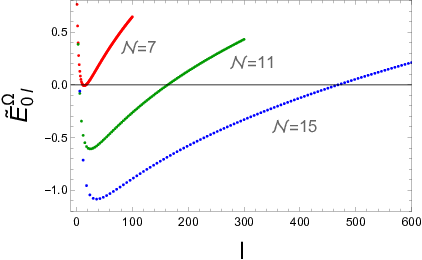
For the purpose of intuition, we show the scaled dimensionless energy

for different values of $\mathcal{N}$ in Fig.1, where positive features can always be identified at large $l$. And with the increasing of $\mathcal{N}$, that is, the enhancement of $eB$ for a given $R$, more $\pi^{+}$ can be condensed as more are trapped in the system. It should be pointed out that finite lower boundaries exist for the total energies of any charged particles.

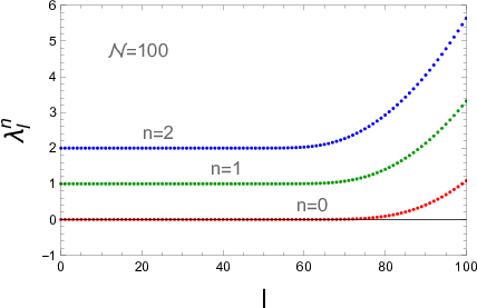
In pure magnetic field, it was found that the degeneracy of $l$ is automatically restricted to $\leq[\mathcal{N}]$ for the lowest Landau level when the boundary condition is applied Chen:2017xrj. We even check in advance that the degeneracy decreases with the Landau level $n$, see the plains in Fig.2. Nevertheless, for the case $\mathcal{N}=15$ in Fig.1, the much wider unstable window of $l$ disfavors the use of the artificial upper bound $[\mathcal{N}]$ for $l$ when large angular velocity ($\Omega\lesssim 1/R$) is involved.

Finally, turn to the charged $\rho$ vector mesons, the story is quite different because of their non-vanishing spins. In the presence of PMR, the effective mass of $\rho^{+}_{\uparrow}$ or $\rho^{-}_{\downarrow}$ decreases as $\sqrt{m_{\rho}^{2}+|eB|(2\lambda_{l}^{0}-1)}$ on one hand Chernodub:2010qx, the effective isospin chemical potential increases as $\Omega(l+1)$ on the other hand. Then, it seems that $\rho^{+}_{\uparrow}$ condensation would overwhelm the $\pi^{+}$ condensation to be the true ground state when $\Omega$ is large enough that

As the VW theorem might forbid the decreasing of composite $\rho^{+}_{\uparrow}$ mass to zero in pure magnetic field Hidaka:2012mz; Bali:2017ian; Cao:2019res; Ding:2020jui, the estimation of the $\rho^{+}_{\uparrow}$ mass is not correct at all for large $B$ in the point particle picture. However, as mentioned in the introduction, $\Omega$ invalids the proof of the theorem thus the isospin chemical potential effect of $\Omega(l+1)$ can still be qualitatively correct in the point particle picture. As a strong support of this point, we’d like to mention that the isospin effect was first discussed in chiral perturbation theory with pions the fundamental degrees of freedom Son:2000xc, and the proposed CPS was well verified by the effective NJL model He:2005nk; Cao:2016ats and lattice QCD simulations Kogut:2002zg; Brandt:2017oyy with quarks the fundamental degrees of freedom.

In order to explore the possibility of charged rho condensation more realistically, we adopt the $SU(3)$ NJL model with $u,d$ and $s$ quarks the fundamental degrees of freedom Klevansky:1992qe. In the rotating frame, the action of the system can be conveniently given in curved spacetime by

where the Lagrangian density can be extended from the usual one Klevansky:1992qe; Klimt:1989pm to

by further adopting the four fermion vector interaction channels with coupling constant $G_{V}$. Compared to the two-flavor NJL model, the advantage of three-flavor NJL model is that there the vacuum superconductivity or CRS cannot happen in pure magnetic field Cao:2019res which is consistent with lattice QCD simulations Hidaka:2012mz; Bali:2017ian; Ding:2020jui.

In the Lagrangian, $\psi=(u,d,s)^{T}$ represents the three-flavor quark field and $m_{0}={\rm diag}(m_{\rm 0u},m_{\rm 0d},m_{\rm 0s})$ is the current quark mass matrix. The longitudinal and transverse covariant derivatives with PMR effect are defined, for symmetric gauge, respectively as

and

with the charge matrix $Q={\rm diag}(q_{\rm u},q_{\rm d},q_{\rm s})$. For the four-fermion interaction terms, $\lambda^{0}=\sqrt{2\over 3}I$ and Gell-Mann matrices $\lambda^{i}~(i=1,\dots,8)$ are defined in three-flavor space, so the extra diagonal terms $(\bar{\psi}\lambda^{3}\psi)^{2}$ and $(\bar{\psi}\lambda^{8}\psi)^{2}$ allow mass splitting among all the flavors in contrary to the two-flavor case Cao:2019res. The $U_{A}(1)$ symmetry violating term ${\cal L}_{6}$ tHooft:1976snw only involves scalar-pseudoscalar channels with the determinant defined in flavor space, $\Gamma^{\pm}=1\pm\gamma_{5}$ and $K$ the coupling constant. Now, we only consider nonzero chiral condensations $\sigma_{\rm i}\equiv\langle\bar{\psi}^{i}{\psi}^{i}\rangle$, where the correspondence between the Arabian denotations $i=1,2,3$ and the more explicit Latin ones ${\rm f=u,d,s}$ should be understood for the flavors. The six fermion interactions in ${\cal L}_{6}$ can be reduced to effective four fermion ones in Hartree approximation Klevansky:1992qe, then the Lagrangian density only involves four fermion effective interactions:

where the non-vanishing elements of the symmetric coupling matrices $G^{\pm}$ are given by Klevansky:1992qe

In the case $\langle\sigma_{i}\rangle\neq 0$, the inverse quark propagators of different flavors are given by the introductions of the dynamical masses and covariant derivatives as

By using the eigenfunction reconstruction method, we have given the propagator of a fermion with positive or negative charge Cao:2019ctl; so the $u$ and $d/s$ quark propagators are respectively

where ${p}_{0}^{ls}=p_{0}+\Omega\left(l+s{1\over 2}\right)$, the dispersion relations $\varepsilon_{n}^{i}=(p_{z}^{2}+2n|q_{i}B|+m_{i}^{2})^{1/2}$ and ${\cal P}_{\uparrow/\downarrow}={1\over 2}(1\pm\sigma^{12})$ are the spin projectors. Here, the normalized auxiliary functions are defined for positive and negative charged particles respectively as

where the dimensionless radius $\tilde{r}^{2}=|qB|r^{2}/2$ and the Laguerre polynomial $L_{n}^{l}(x)$ is nonvanishing only for $n\geq 0$. Actually, in a rotating system, a boundary must be applied due to causality, then the propagators would no longer keeps the forms of Eqs.(12) and (13). But for convenience, we still adopt these forms and constrain the OAM as $l\in\left[-n,\mathcal{N}-n\right]$ Chen:2019tcp. Armed with that, the quark masses can be evaluated through the gap equations given by the self-consistent definitions of chiral condensations as:

By adopting vacuum regularization, the explicit form of the gap equations are

with the reduced cutoff $\tilde{\Lambda}_{\rm f}={\Lambda/m_{\rm f}}$. Compared to that given in Ref. Cao:2019ctl but implicitly implied, the Landau levels are cut off by $n_{\rm max}~(\ll N_{\rm f})$ here, which was checked to be a good approximation for large $B$ and $\Omega=0$.

For a continuous transition, the effective potential can be expressed as the form in Ginzburg-Landau (GL) theory

where $V_{\rm eff}(\sigma_{\rm f},0)$ is the corresponding thermodynamic potential giving rise to the gap equations in Eq.(17). We note that $\Delta$ can be an order parameter for any kind of mesonic superfluid or superconductor with the relevant coefficients ${\cal A}$ and ${\cal B}$ determined by their interactions with quarks. To avoid too much complexity, we assume the transition is solely determined by the quadratic one ${\cal A}$ Cao:2019ctl: If ${\cal A}<0$, the meson condensation is favored; and if ${\cal A}_{a}<{\cal A}_{b}<0$, we would assume meson $a$ is more preferred to condensate than meson $b$. We’ve discovered previously that ${\cal A}$ is almost consistent with the inverse mesonic propagator in random phase approximation (RPA) except for some subtle discussions on the Schwinger phases of charged mesons Cao:2019ctl; Chen:2019tcp; Cao:2015xja. As illuminated in Ref. Cao:2019res, the bare form of the coefficient is given by

with the polarization function defined through the fermion loop as

Here, $V_{4}$ is the space-time volume, the trace should be taken over the internal and coordinate spaces, and $e^{-i\Phi_{M}}$ is the compensated Schwinger phase.

This section is mainly devoted to calculating the quadratic efficient explicitly. The interaction vertices between quarks and (pseudo-)scalar and vector mesons have been listed in Ref. Cao:2019res as:

where $\bar{\gamma}^{\pm}_{\mu}=(\gamma_{0},{\gamma_{1}\pm i\gamma_{2}\over\sqrt{2}},{\gamma_{1}\mp i\gamma_{2}\over\sqrt{2}},\gamma_{3})$. In the following, we mainly focus on the $\bar{\rho}^{+}_{1}$ mode, that is, the rho meson with spin long the magnetic field. The insertion of the fermion propagators from Eq.(17) into the polarization function Eq.(19) is explicitly

References

• (1) V. Skokov, A. Y. Illarionov and V. Toneev, Int. J. Mod. Phys. A 24, 5925 (2009).
• (2) W. T. Deng and X. G. Huang, Phys. Rev. C 85, 044907 (2012).
• (3) X. Guo, J. Liao and E. Wang, Sci. Rep. 10, no.1, 2196 (2020).
• (4) K. Xu, S. Shi, H. Zhang, D. Hou, J. Liao and M. Huang, [arXiv:2004.05362 [hep-ph]].
• (5) Z. T. Liang and X. N. Wang, Phys. Rev. Lett. 94, 102301 (2005).
• (6) F. Becattini, I. Karpenko, M. Lisa, I. Upsal and S. Voloshin, Phys. Rev. C 95, 054902 (2017).
• (7) L. Adamczyk et al. [STAR Collaboration], Nature 548, 62 (2017).
• (8) J. Liao, Pramana 84, no. 5, 901 (2015).
• (9) D. E. Kharzeev, J. Liao, S. A. Voloshin and G. Wang, Prog. Part. Nucl. Phys. 88, 1 (2016).
• (10) X. G. Huang, Rept. Prog. Phys. 79, 076302 (2016).
• (11) J. Adam et al. [STAR Collaboration], arXiv:2006.04251 [nucl-ex].
• (12) V. P. Gusynin, V. A. Miransky and I. A. Shovkovy, Phys. Rev. Lett. 73, 3499 (1994) Erratum: [Phys. Rev. Lett. 76, 1005 (1996)].
• (13) V. P. Gusynin, V. A. Miransky and I. A. Shovkovy, Phys. Lett. B 349, 477 (1995).
• (14) I. Karpenko and F. Becattini, Eur. Phys. J. C 77, 213 (2017).
• (15) H. Li, L. G. Pang, Q. Wang and X. L. Xia, Phys. Rev. C 96, no. 5, 054908 (2017).
• (16) T. Niida [STAR Collaboration], Nucl. Phys. A 982, 511 (2019).
• (17) Y. Guo, S. Shi, S. Feng and J. Liao, Phys. Lett. B 798, 134929 (2019).
• (18) G. S. Bali, F. Bruckmann, G. Endrodi, Z. Fodor, S. D. Katz, S. Krieg, A. Schafer and K. K. Szabo, JHEP 1202, 044 (2012).
• (19) G. S. Bali, F. Bruckmann, G. Endrodi, Z. Fodor, S. D. Katz and A. Schafer, Phys. Rev. D 86, 071502 (2012).
• (20) F. Becattini and I. Karpenko, Phys. Rev. Lett. 120, 012302 (2018).
• (21) X. L. Xia, H. Li, Z. B. Tang and Q. Wang, Phys. Rev. C 98, 024905 (2018).
• (22) F. Becattini, G. Cao and E. Speranza, Eur. Phys. J. C 79 (2019) no.9, 741.
• (23) X. L. Xia, H. Li, X. G. Huang and H. Z. Huang, Phys. Rev. C 100, no. 1, 014913 (2019).
• (24) M. N. Chernodub, Phys. Rev. D 82, 085011 (2010).
• (25) M. N. Chernodub, Phys. Rev. Lett. 106, 142003 (2011).
• (26) G. Cao and X. G. Huang, Phys. Lett. B 757, 1 (2016).
• (27) L. Wang and G. Cao, Phys. Rev. D 97, no. 3, 034014 (2018).
• (28) L. Wang, G. Cao, X. G. Huang and P. Zhuang, Phys. Lett. B 780, 273 (2018).
• (29) G. Cao, Phys. Rev. D 101, no. 9, 094027 (2020).
• (30) Y. Liu and I. Zahed, Phys. Rev. Lett. 120, 032001 (2018).
• (31) V. V. Braguta, P. V. Buividovich, M. N. Chernodub, A. Y. Kotov and M. I. Polikarpov, Phys. Lett. B 718, 667 (2012).
• (32) H. Liu, L. Yu and M. Huang, Phys. Rev. D 91, no. 1, 014017 (2015).
• (33) Y. Hidaka and A. Yamamoto, Phys. Rev. D 87, no. 9, 094502 (2013).
• (34) G. S. Bali, B. B. Brandt, G. Endrodi and B. Glassle, Phys. Rev. D 97, no. 3, 034505 (2018).
• (35) G. Cao, Phys. Rev. D 100, no. 7, 074024 (2019).
• (36) H. T. Ding, S. T. Li, S. Mukherjee, A. Tomiya and X. D. Wang, arXiv:2001.05322 [hep-lat].
• (37) G. Cao and L. He, Phys. Rev. D 100, no. 9, 094015 (2019).
• (38) H. L. Chen, X. G. Huang and K. Mameda, arXiv:1910.02700 [nucl-th].
• (39) C. Vafa and E. Witten, Phys. Rev. Lett. 53, 535 (1984).
• (40) H. Zhang, D. Hou and J. Liao, arXiv:1812.11787 [hep-ph].
• (41) S. Weinberg, Phys. Rev. 166, 1568 (1968).
• (42) T. D. Lee and C. N. Yang, Phys. Rev. 128, 885 (1962).
• (43) H. L. Chen, K. Fukushima, X. G. Huang and K. Mameda, Phys. Rev. D 96, no.5, 054032 (2017).
• (44) Y. Jiang and J. Liao, Phys. Rev. Lett. 117, 192302 (2016).
• (45) P. C. W. Davies, T. Dray and C. A. Manogue, Phys. Rev. D 53, 4382 (1996).
• (46) V. E. Ambrus and E. Winstanley, Phys. Rev. D 93, no. 10, 104014 (2016).
• (47) D. T. Son and M. A. Stephanov, Phys. Rev. Lett. 86, 592 (2001).
• (48) L. y. He, M. Jin and P. f. Zhuang, Phys. Rev. D 71, 116001 (2005).
• (49) G. Cao, L. He and X. G. Huang, Chin. Phys. C 41, no. 5, 051001 (2017).
• (50) J. B. Kogut and D. K. Sinclair, Phys. Rev. D 66, 034505 (2002).
• (51) B. B. Brandt, G. Endrodi and S. Schmalzbauer, Phys. Rev. D 97, no. 5, 054514 (2018).
• (52) S. P. Klevansky, Rev. Mod. Phys. 64, 649 (1992).
• (53) S. Klimt, M. F. M. Lutz, U. Vogl and W. Weise, Nucl. Phys. A 516, 429 (1990).
• (54) G. ’t Hooft, Phys. Rev. D 14, 3432 (1976) Erratum: [Phys. Rev. D 18, 2199 (1978)].
• (55) G. Cao and P. Zhuang, Phys. Rev. D 92, 105030 (2015).
• (56) P. Rehberg, S. P. Klevansky and J. Hufner, Phys. Rev. C 53, 410 (1996).
• (57) L. Wang, Y. Jiang, L. He and P. Zhuang, Phys. Rev. D 100, no.11, 114009 (2019).