∎

A new characterization of symmetric $H^{+}$ -tensors and $M$ -tensors Thanks: This research did not receive any specific grant from funding agencies in the public, commercial, or not-for-profit sectors.

Xin Shi Luis F. Zuluaga

Received: date / Accepted: date

Abstract

In this work, we present a new characterization of symmetric $H^{+}$ -tensors, also referred as generalized diagonally dominant tensors with nonnegative diagonals. Namely, by exploring their diagonal dominance property, we derive new necessary and sufficient conditions for a symmetric tensor to be an $H^{+}$ -tensor. Based on these conditions, we propose a novel method that allows to identify if a tensor is a symmetric $H^{+}$ -tensor in polynomial time, by solving a power cone optimization problem. Further, we show how this result can be used to efficiently compute the minimum $H$ -eigenvalue of symmetric $M$ -tensors and to provide tighter lower bounds for the minimum $H$ -eigenvalue of the Fan product of two symmetric $M$ -tensors. Throughout the article, numerical experiments are used to benchmark and illustrate the applications of our results.

Keywords:

H^{+}

-tensors Generalized Diagonally Dominant tensors Power Cone Optimization Minimum

H

-eigenvalues

MSC

15A69 65F15

1 Introduction

Tensors can be regarded as a high-order generalization of matrices and they arise in applications in many disciplines of science, engineering and social sciences (Landsberg 2012, see, e.g.). For $m,n\in\mathbb{N}$ , an $m$ -order $n$ -dimensional real tensor is a multidimensional array with the form

\mathcal{A}=(a_{i_{1}i_{2}\dots i_{m}}),\quad a_{i_{1}i_{2}\dots i_{m}}\in\mathbb{R},\quad 1\leq i_{1},i_{2},\dots,i_{m}\leq n.

Matrices are tensors with order $m=2$ . Denote $\mathbb{T}_{m,n}$ as the space of all real tensors with order $~m$ and dimension $n$ . Then

\mathbb{T}_{m,n}=\underbrace{\mathbb{R}^{n}\otimes\mathbb{R}^{n}\otimes\cdots\otimes\mathbb{R}^{n}}_{m},

where $\otimes$ is the outer product. Denote $[n]=\{1,2,\dots,n\}$ . Tensor $\mathcal{A}=(a_{i_{1}\dots i_{m}})\in\mathbb{T}_{m,n}$ is called symmetric if its entries $a_{i_{1}\dots i_{m}}$ are invariant under any permutation of $(i_{1},\dots,i_{m})$ for $i_{j}\in[n],j\in[m]$ . Denote $\mathbb{S}_{m,n}$ as the set of symmetric tensors in $\mathbb{T}_{m,n}$ . The entries $a_{ii\dots i}$ for any $i\in[n]$ are called diagonal elements (or entries) of $\mathcal{A}$ .

Following (Cartwright and Sturmfels 2013; Lim 2005; Qi 2005), for $\mathcal{A}\in\mathbb{T}_{m,n}$ , $\lambda\in\mathbb{C}$ is called an eigenvalue of $\mathcal{A}$ , if there exists an eigenvector $x\in\mathbb{C}^{n}\backslash\{0\}$ such that $\mathcal{A}x^{m-1}=\lambda x^{[m-1]}$ , where $\mathcal{A}x^{m-1}\in\mathbb{C}^{n}$ is defined by

\displaystyle(\mathcal{A}x^{m-1})_{i}=\sum_{i_{2},\dots,i_{m}=1}^{n}a_{ii_{2}\dots i_{m}}x_{i_{2}}\cdots x_{i_{m}},

and $x^{[m-1]}\in\mathbb{C}^{n}\backslash\{0\}$ is defined by $(x^{[m-1]})_{i}=x_{i}^{m-1}$ for all $i\in[n]$ . In particular, if $x$ is real, then $\lambda$ is also real. In this case, we say that $\lambda$ is an H-eigenvalue of $\mathcal{A}$ .

The comparison tensor of $\mathcal{A}\in\mathbb{T}_{m,n}$ , denoted as $M(\mathcal{A})$ , is defined in (Ding et al. 2013; Kannan et al. 2015) as follows:

M(\mathcal{A})_{i_{1}\dots i_{m}}=\begin{cases}|a_{i_{1}\dots i_{m}}|&\text{if }i_{1}=\cdots=i_{m},\\ -|a_{i_{1}\dots i_{m}}|&\text{otherwise}.\end{cases}

(1)

Following (Ding et al. 2013; Kannan et al. 2015), we introduce the next classes of tensors. A tensor is called a nonnegative tensor if all its entries are nonnegative and a tensor is called a diagonal tensor if all its off-diagonal elements are zero. A tensor $\mathcal{A}\in\mathbb{T}_{m,n}$ is said to be a $Z$ -tensor if there exists a nonnegative tensor $\mathcal{D}\in\mathbb{T}_{m,n}$ and a nonnegative scalar $s$ such that $\mathcal{A}=s\mathcal{I}-\mathcal{D}$ , where $\mathcal{I}\in\mathbb{T}_{m,n}$ is a diagonal tensor with all diagonal elements equal to one. For tensor $\mathcal{A}$ , denote $\rho(\mathcal{A})$ as the largest modulus of its eigenvalues. A $Z$ -tensor $\mathcal{A}=s\mathcal{I}-\mathcal{D}$ is said to be an $M$ -tensor if $s\geq\rho(\mathcal{D})$ . If $s>\rho(\mathcal{D})$ , then $\mathcal{A}$ is called a strong $M$ -tensor. A tensor is called an $H$ -tensor if its comparison tensor is an $M$ -tensor. From the definition of $M$ -tensors, the diagonal elements of an $M$ -tensor are always nonnegative and the off-diagonal elements are always nonpositive. Thus, the comparison tensor of an $M$ -tensor is always itself. If a tensor is an $M$ -tensor, then it is also an $H$ -tensor with nonnegative diagonal elements. A tensor is called a strong $H$ -tensor if its comparison tensor is a strong $M$ -tensor. An $H$ -tensor with nonnegative diagonal elements is called an $H^{+}$ -tensor. The definition of $H^{+}$ -tensors constitutes a natural generalization of the concept of $H^{+}$ -matrices, as introduced in (Boman et al. 2005) and it matches the definition used in (Luo and Qi 2015) and (Kannan et al. 2015) where they are referred as $H$ -tensors with nonnegative diagonals. Also, as we will discuss later (see Corollary 1 and Definition 1), $H$ -tensors are equivalent to generalized diagonally dominant tensors (Kannan et al. 2015, Thm. 4.9). Thus this definition of $H^{+}$ -tensors also matches with the set of generalized diagonally dominant tensors with nonnegative diagonals in Ahmadi and Majumdar 2019. It is worth noting that in (Wang et al. 2021; Wang et al. 2020a) an alternative definition is used, which does not include $H$ -tensors with $0$ elements in the diagonal. However, our results on identifying $H$ -tensors with nonnegative diagonals can be straightforwardly applied to detect these tensors as well.

A symmetric tensor is an $H$ -tensor if and only if it is a generalized diagonally dominant tensor (Kannan et al. 2015, Thm. 4.9). The matrix version (i.e., when $m$ = 2) of this result is proved in (Boman et al. 2005, Thm. 8) and (Varga and Gillis 1963). As a result, it follows that a symmetric matrix is an $H^{+}$ -matrix if and only if it can be written as the sum of a number of positive semidefinite matrices which have a special sparse structure (Boman et al. 2005). From this fact, it follows that symmetric $H^{+}$ -matrices can be identified in polynomial time by solving a second-order cone optimization (Lobo et al. 1998; Ahmadi and Majumdar 2019, see, e.g.,).

$M$ -tensors and $H$ -tensors have emerged as crucial tools across diverse mathematical and engineering fields, including hypergraph analysis (Fan et al. 2019; Sun et al. 2019; Galuppi et al. 2023), tensor complementarity problems (Huang and Qi 2017; Luo et al. 2017), multilinear systems (Luo et al. 2017; Li and Ng 2015; Ding and Wei 2016; Wang et al. 2019b), optimal control problems (Azimzadeh and Bayraktar 2019), high-order Markov chains (Li and Ng 2014; Liu et al. 2018), and as discussed in detail in Example 3, have the potential to impact results in polynomial optimization. Next, we provide a brief overview of these areas of applications.

•

The Laplacian tensor of a hypergraph is an $M$ -tensor. Researchers are actively investigating the spectral properties of hypergraphs by leveraging the properties of $M$ -tensors (Sun et al. 2019). Specifically, the chromatic number of a hypergraph is bounded using the largest $H$ -eigenvalue of the adjacency tensor (Sun et al. 2019; Cooper and Dutle 2012), which can be determined using the methods proposed in this work. The analysis of properties of hypergraphs, such as their chromatic number, arises when modeling problems in areas as varied as informatics, transportation, molecular biology, and telecommunications, to name just a few (Bretto 2013; Zhang et al. 2016, see, e.g.,). In Example 4, we demonstrate how our method can be used to bound the chromatic number of a hypergraph.
•

Tensor complementarity problems arise in diverse domains, including DNA microarrays, communication systems, and $n$ -person non-cooperative games. Research has shown that solutions to tensor complementarity problems involving $M$ -tensors and $H$ -tensors exhibit desirable properties (Wang et al. 2020a; Luo et al. 2017). In Example 5, we showcase our method’s ability to identify $M$ -tensors in a given problem, which allows us to leverage specialized algorithms to efficiently solve tensor complementarity problems.
•

While analyzing the existence of solutions for general multilinear systems presents significant challenges, the authors in (Ding and Wei 2016; Wang et al. 2019a) have demonstrated the existence of specific solutions for systems involving $M$ -tensors and $H$ -tensors. Furthermore, numerous efficient solution methods have been developed for such systems (Wang et al. 2019b; Wang et al. 2020b). Efficiently characterizing $M$ -tensors and $H$ -tensors facilitates the efficient solution of multilinear systems. In Example 6, we illustrate an application of our method to recognize $M$ -tensors in a multilinear system, enabling the use of specific algorithms to solve the system.
•

For high-order Markov chain models, the transition probability tensors are nonnegative tensors. The problem of determining the limiting probability vectors of these tensors can be addressed by solving a nonlinear equation with $M$ -tensors. The tensor splitting method proposed in (Liu et al. 2018) offers an effective approach to solve such equations. In Example 7, we apply our proposed method to two real-world Markov chain models, demonstrating its effectiveness in obtaining their limiting probability vectors with the tensor splitting method proposed in (Liu et al. 2018).
•

Even order symmetric $H^{+}$ -tensors define globally nonnegative polynomials (Chen et al. 2016a). A recent trend in polynomial optimization (Lasserre 2015) is the derivation of approaches to approximate polynomial optimization problems without the need to use sum of squares polynomials (SOS) (Kuryatnikova et al. 2024; Ahmadi and Majumdar 2019, see, e.g.,). This is mainly motivated by the prohibitively high computational effort needed to solve the semidefinite optimization problems associated with the use of SOS polynomials. As detailed in Example 3, from the results in (Kuryatnikova et al. 2024), it follows that one can construct (convex) power cone optimization-based hierarchies to approximate any polynomial optimization problem with a compact feasible set. This approximation approach demonstrates the potential impact that our results can have in addressing the solution of practically relevant polynomial optimization problems in fields such as statistics and machine learning, derivative pricing, and control theory (Ahmadi and Majumdar 2019).

In this work we generalize the results on symmetric $H^{+}$ matrices to symmetric $H^{+}$ -tensors. Namely, we prove that a symmetric tensor is an $H^{+}$ -tensor if and only if it can be written as the sum of a number of tensors which have a special sparse structure (Theorem 3.3). Based on this, we obtain a novel characterization of symmetric $H^{+}$ -tensors (Theorem 3.4) using conic optimization (Wright 1997, see, e.g.,) techniques. In particular, we show that symmetric $H^{+}$ -tensors can be identified in polynomial time (Corollary 3 and (3.1)) by solving a power cone optimization (Chares 2009; Hien 2015, see, e.g.,) problem.

Many efforts have been made to characterize $H$ -tensors (Huang and Ma 2019a; Li et al. 2014; Li et al. 2017; Liu et al. 2017; Wang et al. 2017; Zhang and Wang 2016; Zhao et al. 2016; Sun 2020; Huang and Ma 2019b; Liu et al. 2020, see, e.g.,), by providing sufficient conditions for a tensor to be an $H$ -tensor. While these algorithms can identify $H^{+}$ -tensors, there remain $H^{+}$ -tensors that elude detection through these methods. An exception is found in (Luan and Zhang 2019), which leverages spectral theory to derive necessary and sufficient conditions for strong $H$ -tensors and introduces an iterative algorithm for their identification with linear convergence. On the other hand, our approach allows us to take advantage of interior point algorithms for power cone optimization, which operate in polynomial time, and achieve at least a linear convergence rate (Chares 2009), to detect symmetric $H^{+}$ -tensors. Furthermore, the sufficient and necessary conditions we present for a symmetric tensor to be an $H^{+}$ -tensor are derived by examining their diagonal dominance properties. This characterization not only facilitates the identification of symmetric $H^{+}$ -tensors but also allows for direct optimization over the set of symmetric $H^{+}$ -tensors. Next, we discuss some advantages of this type of characterization. For that purpose, let us revisit in a bit more detail, one of the applications mentioned earlier.

Consider the problem of computing the minimum $H$ -eigenvalue of symmetric $M$ -tensors, which plays an important role in a wide range of interesting applications (see, Huang et al. 2018, and the references therein). Recent literature (He and Huang 2014; Huang et al. 2018; Li et al. 2013; Tian and Huang 2010) focuses on obtaining bounds on the minimum $H$ -eigenvalue of $M$ -tensors. Our characterization can instead compute the minimum $H$ -eigenvalue of symmetric $M$ -tensors in polynomial time by solving a power cone optimization problem (Corollary 5). Not surprisingly, the values obtained in this way tighten the bounds provided in (He and Huang 2014; Huang et al. 2018; Li et al. 2013; Tian and Huang 2010) (Table 1). Further, the values are computed in a time faster than the one required to compute the minimum $H$ -eigenvalue of $M$ -tensors with a more general algorithm (Chen et al. 2016b) that can be used for this purpose (Table 2). To illustrate the practical applications of these results, we show (Example 4) how to obtain an upper bound on the chromatic number of a hypergraph (Cooper and Dutle 2012, see, e.g.,) by computing the minimum $H$ -eigenvalue of its associated transformed adjacency tensor (Chang et al. 2013, see, e.g.,). As additional applications, in Examples 5, 6, and 7, we demonstrate how computing the minimum $H$ -eigenvalues of $Z$ -tensors enables us to determine whether specialized methods can be applied to find the sparsest solution of a tensor complementarity problem, obtain limiting probability vectors of high-order Markov chains, or, more generally, solve multilinear systems of equations.

Further, consider the problem of finding the minimum $H$ -eigenvalue of the Fan product (Fan 1964) of two symmetric $M$ -tensors. One of the main characteristics of this product is that the Fan product of $M$ -tensors is also an $M$ -tensor (Shen et al. 2019). Some bounds for the minimum $H$ -eigenvalue of the Fan product of $Z$ -matrices ( $Z$ -tensors) are proposed in (Cheng 2014; Fang 2007; Shen et al. 2019). Our characterization can be used to obtain bounds that are theoretically and empirically tighter than any of the bounds provided in (Shen et al. 2019) (Table 4).

The remaining of the article is organized as follows: Section 2 introduces additional notation, definitions and some basic results. In Section 3, the characterizations of symmetric $H^{+}$ -tensors are presented. With these characterizations, we provide a way to identify if a tensor is a symmetric $H^{+}$ -tensor in polynomial time. In Section 4, we show how to obtain the minimum $H$ -eigenvalue of a symmetric $M$ -tensor by applying the methodology proposed in this work. We provide some applications of our characterizations of symmetric $H^{+}$ -tensors and $M$ -tensors in this chapter. In Section 5, we further apply our results to obtain lower bounds for the minimum $H$ -eigenvalue of the Fan product of two symmetric $M$ -tensors, that are tighter than the ones proposed in the related literature. Section 6 concludes the article with some final remarks.

All the computational experiments mentioned in this work were implemented in MATLAB R2022b using the Systems Polynomial Optimization Toolbox (SPOT) (Megretski 2010), and the solver MOSEK 9.3.22 (ApS 2022), using an Intel computer Core i7-4770HQ with 2.20 GHz frequency and 16 GB RAM memory. The packages allcomb(varargin) v4.2 (Jos 2025) and Tensor Toolbox for MATLAB v3.1 (Bader et al. 2019) are also employed to formulate the power cone optimization problems. The Github repository https://github.com/XinEDprob/spotless makes publicly available all the data and code used to generate the computational results presented in the article.

2 Preliminaries

For ease of exposition, in what follows, we use small letters $a,b,\dots$ for scalars and vectors; capital letters $A,B,\dots$ for matrices; calligraphic letters $\mathcal{A},\mathcal{B},\dots$ for tensors and $\mathscr{A},\mathscr{B},\dots$ for index sets; and blackboard bold letters $\mathbb{T},\mathbb{D},\dots$ for other kinds of sets or spaces in this work.

First we introduce additional notation and some fundamental properties of tensors. Let $\mathbb{R}[x]:=\mathbb{R}[x_{1},\dots,x_{n}]$ be the set of polynomials in $n$ variables with real coefficients. A polynomial $p\in\mathbb{R}[x]$ is called a sum of squares (SOS) if it can be written as $p=\sum_{i}q_{i}^{2}$ for a finite number of polynomials $q_{i}\in\mathbb{R}[x]$ . Tensor $\mathcal{A}=(a_{i_{1}i_{2}\dots i_{m}})\in\mathbb{S}_{m,n}$ is said to have an SOS-tensor decomposition if its corresponding polynomial

{\mathcal{A}}x^{m}=\sum_{i_{1},i_{2},\dots,i_{m}=1}^{n}a_{i_{1}i_{2}\dots i_{m}}x_{i_{1}}x_{i_{2}}\cdots x_{i_{m}}

(2)

is an SOS (Luo et al. 2015, see, e.g.,). A tensor is called a PSD tensor if its corresponding polynomial is globally nonnegative (Luo et al. 2015, see, e.g.,). The authors in (Chen et al. 2016a) show that every even order symmetric $H^{+}$ -tensor has an SOS-tensor decomposition.

Theorem 2.1 ((Chen et al. 2016a, Thm. 3.7))

Let $m,n\in\mathbb{N}$ and $\mathcal{A}\in\mathbb{S}_{m,n}$ be an $H^{+}$ -tensor. If $m$ is even, then $\mathcal{A}$ has an SOS-tensor decomposition.

From Theorem 2.1, it follows that an even order symmetric $H^{+}$ -tensor is also a PSD tensor. On the other hand, symmetric $H^{+}$ -tensors can be characterized using the notion of diagonally dominant tensors (see Definition 1). Most of the work related to $H^{+}$ -tensors makes use of the diagonal dominance property (Huang and Ma 2019a; Li et al. 2014; Li et al. 2017; Wang et al. 2017; Zhao et al. 2016, see, e.g.,). We will also make use of this property in our results; hence, we present some related definitions.

Definition 1 ((Luo and Qi 2016, Def. 6.5))

Let $m,n\in\mathbb{N}$ and $\mathcal{A}=(a_{i_{1}\dots i_{m}})\in\mathbb{T}_{m,n}$ .

(i)

$\mathcal{A}$ is called a diagonally dominant (DD) tensor if

$|a_{ii\dots i}|\geq\sum_{(i_{2},\dots,i_{m})\neq(i,\dots,i)}|a_{ii_{2}\dots i_{m}}|,\ \ \forall\ i\in[n].$ (3)

(ii)

$\mathcal{A}$ is called a generalized diagonally dominant (GDD) tensor if there exists a positive diagonal matrix $D$ such that the tensor $\mathcal{A}D^{1-m}D\cdots D$ defined as

(\mathcal{A}D^{1-m}D\cdots D)_{i_{1}\dots i_{m}}=a_{i_{1}\dots i_{m}}d_{i_{1}}^{1-m}d_{i_{2}}\cdots d_{i_{m}},\ \ \forall i_{1},\dots,i_{m}\in[n],

(4)

is diagonally dominant, where $d_{i}=D_{ii}$ is the $i$ th diagonal element of $D$ .

From the definition of DD tensors and GDD tensors, one can derive the following equivalent definition of GDD tensors.

Proposition 1

Let $m,n\in\mathbb{N}$ , then $\mathcal{A}\in\mathbb{T}_{m,n}$ is a GDD tensor if and only if there exists a positive diagonal matrix $D$ such that the tensor $\mathcal{A}DD\dots D$ defined as

(\mathcal{A}DD\cdots D)_{i_{1}\dots i_{m}}=a_{i_{1}\dots i_{m}}d_{i_{1}}d_{i_{2}}\cdots d_{i_{m}},\ \ \forall i_{1},\dots,i_{m}\in[n],

(5)

is diagonally dominant, where $d_{i}=D_{ii}$ is the $i$ th diagonal element of $D$ . If $\mathcal{A}\in\mathbb{S}_{m,n}$ , then $\mathcal{A}DD\cdots D\in\mathbb{S}_{m,n}$ .

Proof

From Definition 1 (ii), if $\mathcal{A}=(a_{i_{1}\dots i_{m}})\in\mathbb{T}_{m,n}$ is a GDD tensor, then there exists a positive diagonal matrix $D$ such that $\mathcal{A}D^{1-m}D\cdots D$ is a DD tensor. That is for all $i\in[n]$ ,

|(\mathcal{A}D^{1-m}D\cdots D)_{i\dots i}|\geq\sum_{(i_{2},\dots,i_{m})\neq(i,\dots,i)}|(\mathcal{A}D^{1-m}D\cdots D)_{ii_{2}\dots i_{m}}|.

(6)

Note that (6) is equivalent to

|a_{i\dots i}|\geq\sum_{(i_{2},\dots,i_{m})\neq(i,\dots,i)}|a_{i\dots i_{m}}d_{i}^{1-m}d_{i_{2}}\cdots d_{i_{m}}|.

(7)

Considering that $d_{i}>0$ for all $i\in[n]$ , and multiplying by $d_{i}^{m}$ on both sides of (7), we have that

|a_{i\dots i}|d_{i}^{m}\geq\sum_{(i_{2},\dots,i_{m})\neq(i,\dots,i)}|a_{i\dots i_{m}}|d_{i}d_{i_{2}}\cdots d_{i_{m}},

(8)

for all $i\in[n]$ . Thus, the tensor $\mathcal{A}DD\dots D$ defined by (5) is a DD tensor.

For the another direction, if the tensor $\mathcal{A}DD\cdots D$ defined by (5) is a DD tensor for a positive diagonal matrix $D$ , then inequality (8) holds for all $i\in[n]$ . Dividing both sides of (8) by $d_{i}^{m}>0$ , we have inequality (7), which is equivalent to (6), for all $i\in[n]$ and shows that $\mathcal{A}$ is a GDD tensor.

For the remainder of the article, denote by ${DD}_{m,n}$ and ${GDD}_{m,n}$ the set of DD tensors and the set of GDD tensors in $\mathbb{S}_{m,n}$ , respectively. DD and GDD tensors with nonnegative diagonal elements will be referred as DD⁺ and GDD⁺ tensors, respectively. Also, denote by $DD^{+}_{m,n}$ and $GDD^{+}_{m,n}$ the set of DD⁺ tensors and the set of GDD⁺ tensors in $\mathbb{S}_{m,n}$ , respectively. The set of PSD tensors in $\mathbb{S}_{m,n}$ is denoted as $PSD_{m,n}$ .

For $n\in\mathbb{N}$ , a set $\mathbb{W}\subset\mathbb{R}^{n}$ is called a cone if $0\in\mathbb{W}$ and $x\in\mathbb{W}$ implies $\lambda x\in\mathbb{W}$ for any $\lambda\geq 0$ . A set $\mathbb{W}$ is called a convex cone if $\lambda x+\mu y\in\mathbb{W}$ for any $x,y\in\mathbb{W}$ and any $\lambda,\mu\geq 0$ . Given a set $\mathbb{W}$ , let $cone(\mathbb{W})=\{\lambda x\ |\ x\in\mathbb{W},\lambda\geq 0\}$ be the conic hull of $\mathbb{W}$ ; and $convex(\mathbb{W})=\{\lambda x+\mu y\ |\ x,y\in\mathbb{W},\lambda,\mu\geq 0,\lambda+\mu=1\}$ be the convex hull of $\mathbb{W}$ .

Clearly, for $m,n\in\mathbb{N}$ , $DD^{+}_{m,n}$ is a convex cone. We will show that $GDD^{+}_{m,n}$ is also a convex cone later (see Proposition 5). Next we present a characterization of symmetric $H$ -tensors via symmetric GDD tensors.

Theorem 2.2 ((Kannan et al. 2015, Thm. 4.9))

Let $m,n\in\mathbb{N}$ and $\mathcal{A}\in\mathbb{S}_{m,n}$ . Then $\mathcal{A}$ is an $H$ -tensor if and only if $\mathcal{A}\in GDD_{m,n}$ .

Corollary 1

Let $m,n\in\mathbb{N}$ and $\mathcal{A}\in\mathbb{S}_{m,n}$ . Then $\mathcal{A}$ is an $H^{+}$ -tensor if and only if $\mathcal{A}\in GDD^{+}_{m,n}$ .

From Theorem 2.1 and Corollary 1, if $m$ is even, we have the following inclusion relationships:

DD^{+}_{m,n}\subseteq GDD^{+}_{m,n}\subseteq PSD_{m,n}.

In light of Corollary 1, in what follows, we will take the liberty to use both symmetric $H^{+}$ and GDD⁺ interchangeably to refer to symmetric $H^{+}$ -tensors.

Denote $\operatorname{card}(A)$ as the cardinality of the set $A$ . For $m,n\in\mathbb{N}$ , define the index sets

\begin{split}\mathscr{D}_{n}^{m}=\{(i_{1},\dots,i_{m})\ |\ 1\leq i_{1}\leq\cdots\leq i_{m}\leq n\}\cap\\ \{(i_{1},\dots,i_{m})\ |\ \operatorname{card}(\{i_{1},\dots,i_{m}\})>1\},\end{split}

and

\mathscr{F}_{n}^{m}=\{(\underbrace{i,i,\dots,i}_{m})\ |\ i\in[n]\}.

For any index $(i_{1},\dots,i_{m})\in\mathscr{D}_{n}^{m}\cup\mathscr{F}_{n}^{m}$ , denote $\mathscr{P}_{i_{1}\dots i_{m}}$ as the set of all permutations of $i_{1},\dots,i_{m}$ and denote

\mathscr{Q}_{i_{1}\dots i_{m}}=\{(\underbrace{p,p,\dots,p}_{m})\ |\ p\in\{i_{1},\dots i_{m}\}\}.

Also, for $(i_{1},\dots,i_{m})\in\mathscr{D}_{n}^{m}\cup\mathscr{F}_{n}^{m}$ , let $\mathbb{D}_{m,n}^{i_{1}\dots i_{m}}\in\mathbb{S}_{m,n}$ be the set of sparse tensors defined as follows:

\begin{split}\mathbb{D}_{m,n}^{i_{1}\dots i_{m}}=\{(a_{j_{1}\dots j_{m}})\in\mathbb{S}_{m,n}\ |\ a_{j_{1}\dots j_{m}}=0\text{ \ if \ }\\ (j_{1},\dots,j_{m})\notin\mathscr{P}_{i_{1}\dots i_{m}}\cup\mathscr{Q}_{i_{1}\dots i_{m}}\}.\end{split}

(9)

Further, let

\mathbb{D}_{m,n}=\bigcup_{(i_{1},\dots,i_{m})\in\mathscr{D}_{n}^{m}}\mathbb{D}_{m,n}^{i_{1}\dots i_{m}}.

To proceed, we introduce the following class of tensors.

Definition 2

For $m,n\in\mathbb{N}$ and any $(i_{1},\dots,i_{m})\in\mathscr{D}_{n}^{m}$ , $c\in\{0,1\}$ , denote $\mathcal{V}^{c,i_{1}\dots i_{m}}=(v^{c,i_{1}\dots i_{m}}_{j_{1}\dots j_{m}})\in\mathbb{D}_{m,n}^{i_{1}\dots i_{m}}$ , as the tensor satisfying:

(i)

$v^{c,i_{1}\dots i_{m}}_{j_{1}\dots j_{m}}=(-1)^{c}$ if $(j_{1},\dots,j_{m})\in\mathscr{P}_{i_{1}\dots i_{m}}$ .

(ii)

The value of $j$ -th diagonal element is equal to the sum of the absolute values of the off-diagonal entries on the $j$ -th slice (the diagonal elements are excluded in the sum); that is

v_{jj\dots j}^{c,i_{1}\dots i_{m}}=\sum_{(j_{2},\dots,j_{m})\neq(j,\dots,j)}|v_{jj_{2}\dots j_{m}}^{c,i_{1}\dots i_{m}}|,\forall\ j\in[n].

Further, for all $i\in[n]$ , denote $\mathcal{V}^{0,ii\dots i}$ as the tensor where the only nonzero entry is $v^{0,ii\dots i}_{ii\dots i}=1$ ; and $\mathcal{V}^{1,ii\dots i}$ as the tensor with all entries set to 0. Also, let $\mathbb{E}_{m,n}=\{\mathcal{V}^{c,i_{1}\dots i_{m}}\ |\ c\in\{0,1\},(i_{1},\dots,i_{m})\in\mathscr{D}_{n}^{m}\cup\mathscr{F}_{n}^{m}\}$ .

From Definition 2, it follows that for all $(i_{1},\dots,i_{m})\in\mathscr{D}_{n}^{m}\cup\mathscr{F}_{n}^{m}$ and $c\in\{0,1\}$ , $\mathcal{V}^{c,i_{1}\dots i_{m}}\in DD_{m,n}^{+}$ . For example, when $m=2$ and $n=4$ , we have

\mathcal{V}^{0,12}=\begin{bmatrix}1&1&0&0\\ 1&1&0&0\\ 0&0&0&0\\ 0&0&0&0\end{bmatrix},\quad\quad\mathcal{V}^{1,13}=\begin{bmatrix}1&0&-1&0\\ 0&0&0&0\\ -1&0&1&0\\ 0&0&0&0\end{bmatrix}.\quad\quad

For ease of exposition, we also introduce an auxiliary notation for indices. For $m,n\in\mathbb{N}$ , index ${\vec{i}}:=(i_{1},i_{2},\dots,i_{m})\in\mathscr{D}_{n}^{m}$ and some $l^{{\vec{i}}}\in[m]$ , we call

(({j_{1}^{{\vec{i}}},j_{2}^{{\vec{i}}},\dots,j^{{\vec{i}}}_{l^{{\vec{i}}}}}),({\alpha_{1}^{{\vec{i}}},\alpha_{2}^{{\vec{i}}},\dots,\alpha^{{\vec{i}}}_{l^{{\vec{i}}}}}))\in{[n]^{l^{{\vec{i}}}}\times[m]^{l^{{\vec{i}}}}}

as the tight pair of ${\vec{i}}$ if $({j_{1}^{{\vec{i}}},j_{2}^{{\vec{i}}},\dots,j^{{\vec{i}}}_{l^{{\vec{i}}}}})$ and $({\alpha_{1}^{{\vec{i}}},\alpha_{2}^{{\vec{i}}},\dots,\alpha^{{\vec{i}}}_{l^{{\vec{i}}}}})$ satisfy

x_{i_{1}}x_{i_{2}}\dots x_{i_{m}}=x_{j_{1}^{{\vec{i}}}}^{\alpha_{1}^{{\vec{i}}}}x_{j_{2}^{{\vec{i}}}}^{\alpha_{2}^{{\vec{i}}}}\dots x_{j_{l^{{\vec{i}}}}^{{\vec{i}}}}^{\alpha_{l^{{\vec{i}}}}^{{\vec{i}}}},

(10)

where $1\leq j_{1}^{{\vec{i}}}<j_{2}^{{\vec{i}}}<\dots<j_{l^{{\vec{i}}}}^{{\vec{i}}}\leq n$ . We will refer to $({j_{1}^{{\vec{i}}},j_{2}^{{\vec{i}}},\dots,j^{{\vec{i}}}_{l^{{\vec{i}}}}})$ as the tight index and to $({\alpha_{1}^{{\vec{i}}},\alpha_{2}^{{\vec{i}}},\dots,\alpha^{{\vec{i}}}_{l^{{\vec{i}}}}})$ as the tight power.

The following example illustrates the tight pair notation and shows the benefit of introducing it.

Example 1

Assume index ${\vec{i}}=(i_{1},i_{2},i_{3},i_{4},i_{5},i_{6})=(1,1,1,2,2,3)\in\mathscr{D}_{3}^{6}$ , then the tight index of ${\vec{i}}$ is $(j_{1}^{{\vec{i}}},j_{2}^{{\vec{i}}},j_{3}^{{\vec{i}}})=(1,2,3)$ and the tight power of ${\vec{i}}$ is $(\alpha_{1}^{{\vec{i}}},\alpha_{2}^{{\vec{i}}},\alpha_{2}^{{\vec{i}}})=(3,2,1)$ as

x_{i_{1}}x_{i_{2}}x_{i_{3}}x_{i_{4}}x_{i_{5}}x_{i_{6}}=x_{1}^{3}x_{2}^{2}x_{3}.

Let $\mathcal{A}=(a_{i_{1}i_{2}i_{3}i_{4}i_{5}i_{6}})\in\mathbb{S}_{6,3}$ , one can easily obtain that the coefficient of $x_{1}^{3}x_{2}^{2}x_{3}$ in the corresponding polynomial $\mathcal{A}x^{m}$ is

\binom{m}{\alpha_{1}^{{\vec{i}}},\alpha_{2}^{{\vec{i}}},\alpha_{3}^{{\vec{i}}}}a_{111223}=\binom{6}{3,2,1}a_{111223}.

Besides, it is clear that the element $a_{111223}$ in $\mathcal{A}$ is multiplied by $x_{1}^{3}x_{2}^{2}x_{3}$ in the polynomial $\mathcal{A}x^{m}$ .

It is important to note, however, that we will routinely drop the upper index $\vec{i}$ in the notation when the $\vec{i}$ we are referring to is clear from (or fixed in) the context. Further, denote $e_{j}$ as the unitary vector in the $j$ th direction of appropriate dimensions.

3 New characterization of symmetric $H^{+}$ -tensors

In this section, we present a new characterization of symmetric $H^{+}$ -tensors, or equivalently GDD⁺ tensors (cf., Corollary 1), based on the power cone (Chares 2009; Hien 2015). First, we characterize the set of DD⁺ tensors.

Proposition 2

For $m,n\in\mathbb{N}$ , $DD^{+}_{m,n}=convex(cone(\mathbb{E}_{m,n}))$ and each tensor in $\mathbb{E}_{m,n}$ generates an extreme ray of $DD^{+}_{m,n}$ .

Proof

First, from Definition 2, it follows that $\mathbb{E}_{m,n}\subseteq DD^{+}_{m,n}$ . This, together with the fact that $DD_{m,n}^{+}$ is a convex cone, implies that $convex(cone(\mathbb{E}_{m,n}))\subseteq DD^{+}_{m,n}$ .

Second, for $\mathcal{A}=(a_{i_{1}\dots i_{m}})\in DD^{+}_{m,n}$ , denote

\mathscr{P}_{+}=\{(i_{1},\dots,i_{m})\in\mathscr{D}_{n}^{m}\ |\ a_{i_{1}i_{2}\dots i_{m}}\geq 0\}

and

\mathscr{P}_{-}=\{(i_{1},\dots,i_{m})\in\mathscr{D}_{n}^{m}\ |\ a_{i_{1}i_{2}\dots i_{m}}<0\}.

Then

	$\displaystyle\mathcal{A}=$	$\displaystyle\sum_{i=1}^{n}\left(a_{ii\dots i}-\sum_{(i_{2},\dots,i_{m})\neq(i,\dots,i)}\|a_{ii_{2}\dots i_{m}}\|\right)\mathcal{V}^{0,ii\dots i}$		(11)
	$\displaystyle+$	$\displaystyle\sum_{(i_{1},i_{2},\dots,i_{m})\in\mathscr{P}_{+}}a_{i_{1}i_{2}\dots i_{m}}\mathcal{V}^{0,i_{1}i_{2}\dots i_{m}}+\sum_{(i_{1},i_{2},\dots,i_{m})\in\mathscr{P}_{-}}(-a_{i_{1}i_{2}\dots i_{m}})\mathcal{V}^{1,i_{1}i_{2}\dots i_{m}}.$

Since $\mathcal{A}\in DD_{m,n}^{+}$ , $a_{ii\dots i}\geq\sum_{(i_{2},\dots,i_{m})\neq(i,\dots,i)}|a_{ii_{2}\dots i_{m}}|$ for all $i\in[n]$ . Thus, $\mathcal{A}$ is in the convex hull of the conic hull of $\mathbb{E}_{m,n}$ , after noticing that all the coefficients in the right hand side of (11) are nonnegative. That is $DD^{+}_{m,n}\subseteq convex(cone(\mathbb{E}_{m,n}))$ .

To give a similar characterization for GDD⁺ tensors, we need the following results first.

Theorem 3.1 ((Qi 2013, Thm. 1(a)))

For $m,n\in\mathbb{N}$ , if $\mathcal{D}\in\mathbb{S}_{m,n}$ is a nonnegative tensor, then $\rho(\mathcal{D})$ is an $H$ -eigenvalue of $\mathcal{D}$ .

Denote the largest $H$ -eigenvalue of tensor $\mathcal{A}\in\mathbb{S}_{m,n}$ as $\lambda_{\max}(\mathcal{A})$ .

Theorem 3.2 ((Qi 2013, Thm. 2))

For $m,n\in\mathbb{N}$ , if $\mathcal{A}\in\mathbb{S}_{m,n}$ is a nonnegative tensor, then

\lambda_{\max}(\mathcal{A})={\max}\left\{\mathcal{A}x^{m}:x\in\mathbb{R}^{n}_{+},\sum_{i=1}^{n}x_{i}^{m}=1\right\}.

Using an approach similar to the one used to prove (Zhang et al. 2014, Thm. 4.5), we can establish a slight generalization of that result in Proposition 3.

Proposition 3

For $m,n\in\mathbb{N}$ , if both $\mathcal{A}\in\mathbb{S}_{m,n}$ and $\mathcal{B}\in\mathbb{S}_{m,n}$ are nonnegative tensors, then $\rho(\mathcal{A}+\mathcal{B})\leq\rho(\mathcal{A})+\rho(\mathcal{B})$ .

Proof

Let $\mathcal{D}\in\mathbb{T}_{m,n}$ . From the definition of $\rho(\mathcal{D})$ and $\lambda_{\max}(\mathcal{D})$ , it clearly follows that $\rho(\mathcal{D})\geq\lambda_{\max}(\mathcal{D})$ . If $\mathcal{D}$ is a symmetric nonnegative tensor, it then follows from Theorem 3.1 that

\rho(\mathcal{D})=\lambda_{\max}(\mathcal{D}).

(12)

Let $\mathcal{A}\in\mathbb{S}_{m,n}$ , and $\mathcal{B}\in\mathbb{S}_{m,n}$ be nonnegative tensors. Then we have from equation (12) that $\rho(\mathcal{A})=\lambda_{\max}(\mathcal{A})$ and $\rho(\mathcal{B})=\lambda_{\max}(\mathcal{B})$ . Furthermore, it follows from Theorem 3.2 that

	$\displaystyle\lambda_{\max}(\mathcal{A}+\mathcal{B})$	$\displaystyle={\max}\left\{(\mathcal{A}+\mathcal{B})x^{m}:x\in\mathbb{R}^{n}_{+},\sum_{i=1}^{n}x_{i}^{m}=1\right\}$
		$\displaystyle={\max}\left\{\mathcal{A}x^{m}+\mathcal{B}y^{m}:x,y\in\mathbb{R}^{n}_{+},\sum_{i=1}^{n}x_{i}^{m}=1,\sum_{i=1}^{n}y_{i}^{m}=1,x=y\right\}$
		$\displaystyle\leq{\max}\left\{\mathcal{A}x^{m}:x\in\mathbb{R}^{n}_{+},\sum_{i=1}^{n}x_{i}^{m}=1\right\}$
		$\displaystyle\quad+{\max}\left\{\mathcal{B}y^{m}:y\in\mathbb{R}^{n}_{+},\sum_{i=1}^{n}y_{i}^{m}=1\right\}$
		$\displaystyle=\lambda_{\max}(\mathcal{A})+\lambda_{\max}(\mathcal{B}).$

To finish, notice that $\mathcal{A}+\mathcal{B}$ is a symmetric nonnegative tensor. Thus after using equation (12) for the tensor $\mathcal{A}+\mathcal{B}$ , we conclude that $\rho(\mathcal{A}+\mathcal{B})=\lambda_{\max}(\mathcal{A}+\mathcal{B})\leq\lambda_{\max}(\mathcal{A})+\lambda_{\max}(\mathcal{B})=\rho(\mathcal{A})+\rho(\mathcal{B})$ .

Proposition 4 ((Kannan et al. 2015, Prop. 2.7))

For $m,n\in\mathbb{N}$ , let $\mathcal{B}\in\mathbb{S}_{m,n}$ be a $Z$ -tensor such that $\mathcal{A}\leq\mathcal{B}$ where $\mathcal{A}$ is an $M$ -tensor. Then $\mathcal{B}$ is also an $M$ -tensor.

Proposition 5

For $m,n\in\mathbb{N}$ , $GDD_{m,n}^{+}$ is a convex cone.

Proof

Let $\mathcal{A}=(a_{i_{1}\dots i_{m}})\in GDD_{m,n}^{+}$ and $\mathcal{B}=(b_{i_{1}\dots i_{m}})\in GDD_{m,n}^{+}$ . From Corollary 1, both $\mathcal{A}$ and $\mathcal{B}$ are symmetric $H^{+}$ -tensors. Thus $M(\mathcal{A})$ and $M(\mathcal{B})$ are symmetric $M$ -tensors. That is, there exist nonnegative scalars $s_{1},s_{2}$ and nonnegative tensors $\mathcal{D}_{1}$ and $\mathcal{D}_{2}$ such that $M(\mathcal{A})=s_{1}I-\mathcal{D}_{1}$ , $M(\mathcal{B})=s_{2}I-\mathcal{D}_{2}$ and $s_{1}\geq\rho(\mathcal{D}_{1})$ , $s_{2}\geq\rho(\mathcal{D}_{2})$ . Then $M(\mathcal{A})+M(\mathcal{B})=(s_{1}+s_{2})I-(\mathcal{D}_{1}+\mathcal{D}_{2})$ . Since $s_{1}+s_{2}\geq 0$ and $D_{1}+D_{2}$ is a nonnegative tensor, $M(\mathcal{A})+M(\mathcal{B})$ is a symmetric $Z$ -tensor. Also, from Proposition 3, if follows that $\rho(\mathcal{D}_{1}+\mathcal{D}_{2})\leq\rho(\mathcal{D}_{1})+\rho(\mathcal{D}_{2})\leq s_{1}+s_{2}$ . Thus, $M(\mathcal{A})+M(\mathcal{B})$ is also a symmetric $M$ -tensor.

Next, we prove that $M(\mathcal{A}+\mathcal{B})$ is a $Z$ -tensor. Recall that $M(\mathcal{A}+\mathcal{B})$ is the comparison matrix of $\mathcal{A}+\mathcal{B}$ . Thus, all its diagonal elements are nonnegative and all off-diagonal elements are nonpositive. Denote $s={\max}\{|a_{ii\dots i}|+|b_{ii\dots i}|,i\in[n]\}$ . Then $M(\mathcal{A}+\mathcal{B})=sI-(sI-M(\mathcal{A}+\mathcal{B}))$ where $sI-M(\mathcal{A}+\mathcal{B})$ is a nonnegative tensor. Thus, $M(\mathcal{A}+\mathcal{B})$ is a $Z$ -tensor.

From the definition of comparison tensors and the fact that $\mathcal{A},\mathcal{B}$ have nonnegative diagonal elements, $M(\mathcal{A}+\mathcal{B})\geq M(\mathcal{A})+M(\mathcal{B})$ componentwise. From the fact that $M(\mathcal{A})+M(\mathcal{B})$ is an $M$ -tensor and $M(\mathcal{A}+\mathcal{B})$ is a $Z$ -tensor, it follows from Proposition 4 that $M(\mathcal{A}+\mathcal{B})$ is also an $M$ -tensor. Thus $\mathcal{A}+\mathcal{B}$ is a symmetric $H^{+}$ -tensor, and from Corollary 1, $\mathcal{A}+\mathcal{B}$ is a GDD⁺ tensor. Thus, $\mathcal{A}+\mathcal{B}\in GDD_{m,n}^{+}$ . This, together with the fact that $\mathcal{A}\in GDD_{m,n}^{+}$ implies $\lambda\mathcal{A}\in GDD_{m,n}^{+}$ for any nonnegative scalar $\lambda$ , implies that $GDD_{m,n}^{+}$ is a convex cone.

Theorem 3.3

For $m,n\in\mathbb{N}$ , $\mathcal{A}\in GDD_{m,n}^{+}$ if and only if $\mathcal{A}=\sum_{i=1}^{r}B_{i}$ where $r\in\mathbb{N}$ and $B_{i}\in\mathbb{D}_{m,n}\cap GDD_{m,n}^{+}$ .

Proof

For $m,n\in\mathbb{N}$ , let $\mathcal{A}\in GDD^{+}_{m,n}$ . Then, from Proposition 1, there exists a positive diagonal matrix $D$ such that $\mathcal{B}:=\mathcal{A}DD\cdots D\in DD^{+}_{m,n}$ . From Proposition 2, it follows that there exist $r\in\mathbb{N}$ , $\lambda_{i}\geq 0$ , $\mathcal{C}_{i}\in\mathbb{E}_{m,n}\subset\mathbb{D}_{m,n}\cap DD_{m,n}^{+}$ for $i\in[r]$ such that $\mathcal{B}=\sum_{i=1}^{r}\lambda_{i}\mathcal{C}_{i}$ . Then $\mathcal{A}=\sum_{i=1}^{r}\lambda_{i}\mathcal{C}_{i}D^{-1}\cdots D^{-1}D^{-1}$ . Let $\mathcal{B}_{i}=\lambda_{i}\mathcal{C}_{i}D^{-1}\cdots D^{-1}D^{-1}$ for all $i\in[r]$ . Then the only if statement follows after noticing that for all $i\in[r]$ , $\mathcal{B}_{i}\in GDD_{m,n}^{+}$ and $\mathcal{B}_{i}\in\mathbb{D}_{m,n}$ (as multiplying with positive numbers will not affect the sparse structure of tensors $\mathcal{C}_{i}\in\mathbb{D}_{m,n}$ , $i\in[r]$ ). For the if statement, note that if $\mathcal{A}=\sum_{i=1}^{r}\mathcal{B}_{i}$ with $\mathcal{B}_{i}\in\mathbb{D}_{m,n}^{+}\cap GDD_{m,n}^{+}$ for all $i\in[r]$ , then, from Proposition 5, we have $\mathcal{A}\in GDD_{m,n}^{+}$ .

The matrix version (i.e. $m=2$ ) of Theorem 3.3 was presented in (Ahmadi and Majumdar 2019; Boman et al. 2005).

Lemma 1 ((Ahmadi and Majumdar 2019, Lem. 3.8))

For $n\in\mathbb{N}$ , if matrix $A\in\mathbb{S}_{2,n}$ , then $A$ is a GDD⁺ matrix if and only if $A=\sum_{i<j}M^{ij}$ where each $M^{ij}\in\mathbb{S}_{2,n}$ with zeros everywhere except for four entries $(M^{ij})_{ii}$ , $(M^{ij})_{ij}$ , $(M^{ij})_{ji}$ , $(M^{ij})_{jj}$ which make $M^{ij}$ symmetric and positive semidefinite.

It is easy to see that $M^{ij}$ in Lemma 1 is positive semidefinite if and only if $M^{ij}$ is a GDD⁺ matrix. Thus, Lemma 1 can be regarded as a special case of Theorem 3.3. In Theorem 3.4, we provide sufficient and necessary conditions for a tensor to be in $\mathbb{D}_{m,n}\cap GDD_{m,n}^{+}$ (i.e., a sparse GDD⁺ tensor).

Theorem 3.4

Let $m,n\in\mathbb{N}$ , $(i_{1},\dots,i_{m})\in\mathscr{D}_{n}^{m}\cup\mathscr{F}_{n}^{m}$ , and a tensor $\mathcal{B}=(b_{p_{1}\dots p_{m}})\in\mathbb{D}^{i_{1}\dots i_{m}}_{m,n}$ be given. Then,

(i)

if $(i_{1},\dots,i_{m})\in\mathscr{D}_{n}^{m}$ , $\mathcal{B}\in GDD^{+}_{m,n}$ if and only if its entries satisfy

$\prod_{k=1}^{l}b_{j_{k}j_{k}\dots j_{k}}^{\alpha_{k}}\geq c|b_{i_{1}\dots i_{m}}|^{m},$ (13)

where $c=\prod_{k=1}^{l}{\binom{m-1}{\alpha-e_{k}}}^{\alpha_{k}}$ , and $((j_{1},\dots,j_{l}),\alpha=(\alpha_{1},\dots.\alpha_{l}))$ is the tight pair associated with $(i_{1},\dots,i_{m})$ , and

$b_{pp\dots p}\geq 0,\quad\forall\ (p,p,\dots,p)\in\mathscr{Q}_{i_{1}\dots i_{m}}.$ (14)
(ii)

if $(i_{1},\dots,i_{m})\in\mathscr{F}_{n}^{m}$ , $\mathcal{B}\in GDD^{+}_{m,n}$ if and only if $\mathcal{B}$ is a diagonal tensor satisfying $b_{i_{1}\dots i_{m}}\geq 0$ .

Proof

Let $(i_{1},\dots,i_{m})\in\mathscr{D}_{n}^{m}$ be given. Denote $((j_{1},\dots,j_{l}),\alpha=(\alpha_{1},\dots.\alpha_{l}))$ as the tight pair associated with $(i_{1},\dots,i_{m})$ . Let $\mathcal{B}\in\mathbb{D}^{i_{1}\dots i_{m}}_{m,n}$ . Then, all the off-diagonal elements of $\mathcal{B}$ are zero except for the elements $b_{p_{1}\dots p_{m}}$ , where $(p_{1},\dots,p_{m})\in\mathscr{P}_{i_{1}\dots i_{m}}$ . Then, using Proposition 1, it follows that $\mathcal{B}\in GDD_{m,n}^{+}$ if and only if its entries satisfy (14) and

b_{j_{k}j_{k}\dots j_{k}}d_{j_{k}}^{m}\geq\binom{m-1}{\alpha-e_{k}}|b_{i_{1}\dots i_{m}}|d_{i_{1}}d_{i_{2}}\dots d_{i_{m}},

(15)

for $k\in[l]$ and some $d_{j_{k}}>0$ , for all $k\in[l]$ , after using (8), the sparsity pattern and symmetry of $\mathcal{B}$ , and the fact that the number of equal summands in the right-hand side of (8) in this case is $\binom{m-1}{\alpha-e_{k}}$ .

Now note that if (14) and (15) hold then (14) and

b_{j_{k}j_{k}\dots j_{k}}^{\alpha_{k}}d_{j_{k}}^{m\alpha_{k}}\geq\binom{m-1}{\alpha-e_{k}}^{\alpha_{k}}|b_{i_{1}\dots i_{m}}|^{\alpha_{k}}d_{i_{1}}^{\alpha_{k}}d_{i_{2}}^{\alpha_{k}}\dots d_{i_{m}}^{\alpha_{k}},

(16)

hold for all $k\in[l]$ , and some $d_{j_{k}}>0$ , for all $k\in[l]$ ; since (16) is obtained by taking the $\alpha_{k}$ th power on both sides of (15), whose (multiplicative) terms are all nonnegative. Given that both the left-hand side and the right-hand side of (16) are nonnegative, it follows, after multiplying the left-hand sides and the right-hand sides of (16) for all $k\in[l]$ , and using the fact that $\|\alpha\|_{1}=m$ , that (14) and (16) imply (14) and

\prod_{k=1}^{l}(b_{j_{k}j_{k}\dots j_{k}}^{\alpha_{k}}d_{j_{k}}^{m\alpha_{k}})\geq\left(\prod_{k=1}^{l}\binom{m-1}{\alpha-e_{k}}^{\alpha_{k}}\right)|b_{i_{1}\dots i_{m}}|^{m}(d_{i_{1}}d_{i_{2}}\dots d_{i_{m}})^{m},

(17)

for some $d_{j_{k}}>0$ , for all $k\in[l]$ . In turn, (17) is equivalent to (13), with $c:=\prod_{k=1}^{l}\binom{m-1}{\alpha-e_{k}}^{\alpha_{k}}$ , after noticing that from the definition of tight pair (10), it follows that

\prod_{k=1}^{l}d_{j_{k}}^{\alpha_{k}}=d_{i_{1}}d_{i_{2}}\dots d_{i_{m}}.

(18)

Now, to complete the proof, we show that (13) and (14) imply (15) (i.e., that $\mathcal{B}$ is a $GDD^{+}_{m,n}$ tensor). First note that if for any $k\in[l]$ , $b_{j_{k}j_{k}\dots j_{k}}=0$ , then (13) implies that $b_{i_{1}\dots i_{m}}=0$ . Thus, in this case, given (14) and the fact that $d_{j_{k}}>0$ for all $k\in[l]$ , it follows that (15) is satisfied for all $k\in[l]$ . Moreover, in the case where $b_{i_{1}\dots i_{m}}=0$ , condition (15) follows from (14), given the fact that $d_{j_{k}}>0$ for all $k\in[l]$ . Thus, it is enough to consider the case in which $b_{j_{k}j_{k}\dots j_{k}}>0$ for all $k\in[l]$ , and $b_{i_{1}\dots i_{m}}\not=0$ . In this case, using the fact that $d_{j_{k}}>0$ , we can write that

d_{j_{k}}=z\sqrt[m]{\frac{\binom{m-1}{\alpha-e_{k}}}{b_{j_{k}j_{k}\dots j_{k}}}},

(19)

for some $z>0$ , for all $k\in[l]$ . Thus, for any $k\in[l]$ , it follows that

|b_{i_{1}\dots i_{m}}|d_{i_{1}}\dots d_{i_{m}}=z^{m}|b_{i_{1}\dots i_{m}}|\sqrt[m]{\frac{c}{\Pi_{k=1}^{l}b_{j_{k}j_{k}\dots j_{k}}^{\alpha_{k}}}}\leq z^{m}=\frac{b_{j_{k}j_{k}\dots j_{k}}d_{j_{k}}^{m}}{\binom{m-1}{\alpha-e_{k}}},

(20)

where the first equality follows by using (18), (19), and the definition of $c$ ; the inequality follows from (13), and the last equality follows by using (19) again. After noticing that (20) is equivalent to (15), it then follows that (13) and (14) imply (15); that is, that $\mathcal{B}\in GDD^{+}_{n,m}$ .

If $(i_{1},\dots,i_{m})\in\mathscr{F}_{n}^{m}$ and tensor $\mathcal{B}=(b_{p_{1}\dots p_{m}})\in\mathbb{D}^{i_{1}\dots i_{m}}_{m,n}$ , it follows from the definition of $\mathbb{D}^{i_{1}\dots i_{m}}_{m,n}$ (i.e., (9)) that $\mathcal{B}$ is a diagonal tensor in which the only nonzero entry is $b_{i_{1}\dots i_{m}}$ . Thus, $\mathcal{B}\in GDD^{+}_{m,n}$ tensor if and only if $\mathcal{B}$ is a diagonal tensor satisfying $b_{i_{1}\dots i_{m}}\geq 0$ .

Next, in Corollary 2, we apply Theorem 3.3 and Theorem 3.4 to obtain sufficient and necessary conditions for a tensor $\mathcal{A}\in\mathbb{S}_{m,n}$ to be an $H^{+}$ -tensor (or equivalently a GDD⁺ tensor). Efforts to characterize $H$ -tensors (Huang and Ma 2019a; Li et al. 2014; Li et al. 2017; Liu et al. 2017; Wang et al. 2017; Zhang and Wang 2016; Zhao et al. 2016; Sun 2020; Huang and Ma 2019b; Liu et al. 2020, see, e.g.,) have focused on establishing sufficient conditions for a tensor to qualify as such. While these existing algorithms can detect many $H^{+}$ -tensors, some evade detection. Notably, (Luan and Zhang 2019) employs spectral theory to derive a necessary and sufficient condition for strong $H$ -tensors, offering an iterative method with linear convergence. In contrast, building upon Corollary 2, our approach allows us to take advantage of interior point methods for power cone optimization, ensuring polynomial time complexity and at least linear convergence (Chares 2009). These conditions, derived from diagonal dominance properties, not only aid in identifying symmetric $H^{+}$ -tensors but also enable direct optimization within this tensor class, highlighting the strengths of our method.

Corollary 2

Let $m,n\in\mathbb{N}$ . Then $\mathcal{A}=(a_{p_{1}p_{2}\dots p_{m}})\in\mathbb{S}_{m,n}$ is a GDD⁺ tensor if and only if there exist $b^{\vec{i}}_{j}\geq 0$ for all $\vec{i}=(i_{1},\dots,i_{m})\in\mathscr{D}_{n}^{m}$ , $j\in{\vec{i}}$ satisfying

(i)

For $\vec{i}\in\mathscr{D}_{n}^{m}$ ,

$\prod_{k=1}^{l^{{\vec{i}}}}(b^{{\vec{i}}}_{j_{k}})^{\alpha_{k}^{{\vec{i}}}}\geq c({\vec{i}})|a_{\vec{i}}|^{m}$ (21)

where $c({\vec{i}})=\prod_{k=1}^{l^{\vec{i}}}{\binom{m-1}{\alpha^{\vec{i}}-e_{k}}}^{\alpha^{\vec{i}}_{k}}$ , and $((j^{\vec{i}}_{1},j^{\vec{i}}_{2},\dots,j^{\vec{i}}_{l^{\vec{i}}}),\alpha^{\vec{i}}=(\alpha^{\vec{i}}_{1},\alpha^{\vec{i}}_{2},\dots.\alpha^{\vec{i}}_{l^{\vec{i}}}))$ is the tight pair associated with $\vec{i}$ .
(ii)

For $j\in[n]$ ,

$a_{jj\dots j}\geq\sum_{\vec{i}\in\mathscr{D}_{n}^{m}:j\in\vec{i}}b^{\vec{i}}_{j}.$ (22)

Proof

Let $m,n\in\mathbb{N}$ . From Theorem 3.3, $\mathcal{A}=(a_{p_{1}p_{2}\dots p_{m}})\in\mathbb{S}_{m,n}$ is a GDD⁺ tensor if and only if

\mathcal{A}=\sum_{\vec{i}\in\mathscr{D}_{n}^{m}\cup\mathscr{F}_{n}^{m}}\mathcal{B}^{{\vec{i}}}

(23)

and for $\vec{i}\in\mathscr{D}_{n}^{m}\cup\mathscr{F}_{n}^{m}$ , $\mathcal{B}^{{\vec{i}}}=(b^{{\vec{i}}}_{p_{1}p_{2}\dots p_{m}})\in\mathbb{D}_{m,n}\cap GDD_{m,n}^{+}$ satisfies conditions 14 and (ii) in Theorem 3.4. Note that from the sparse structure of the tensors $\mathcal{B}^{\vec{i}}$ used in (23), it follows that for any $j\in[n]$ ,

a_{jj\dots j}=\sum_{\vec{i}\in\mathscr{D}_{n}^{m}:(j,j,\dots,j)\in\mathscr{Q}_{\vec{i}}}b^{\vec{i}}_{jj\dots j}+b^{jj\dots j}_{jj\dots j},

(24)

and for any $\vec{i}\in\mathscr{D}_{n}^{m}$ ,

a_{\vec{i}}=b^{\vec{i}}_{\vec{i}}.

(25)

From Theorem 3.4 14 and (25), it follows that

c({\vec{i}})|a_{\vec{i}}|^{m}=c({\vec{i}})|b^{\vec{i}}_{\vec{i}}|^{m}\leq\prod_{k=1}^{l^{{\vec{i}}}}(b^{{\vec{i}}}_{j_{k}j_{k}\dots j_{k}})^{\alpha_{k}^{{\vec{i}}}}

where $c({\vec{i}})=\prod_{k=1}^{l^{\vec{i}}}{\binom{m-1}{\alpha^{\vec{i}}-e_{k}}}^{\alpha^{\vec{i}}_{k}}$ , $((j^{\vec{i}}_{1},j^{\vec{i}}_{2},\dots,j^{\vec{i}}_{l^{\vec{i}}}),\alpha^{\vec{i}}=(\alpha^{\vec{i}}_{1},\alpha^{\vec{i}}_{2},\dots.\alpha^{\vec{i}}_{l^{\vec{i}}}))$ is the tight pair associated with $\vec{i}$ , and $b^{{\vec{i}}}_{pp\dots p}\geq 0$ , for all $(p,p,\dots,p)\in\mathscr{Q}_{{\vec{i}}}$ . The statement then follows from this and (24), after noticing that from Theorem 3.4 (ii), $b^{jj\dots j}_{jj\dots j}\geq 0$ for all $j\in[n]$ , and after simplifying notation to let $b^{\vec{i}}_{jj\dots j}:=b^{\vec{i}}_{j}$ for any $\vec{i}\in\mathscr{D}_{n}^{m}:(jj\dots j)\in\mathscr{Q}_{\vec{i}}$ ; that is, for any $\vec{i}\in\mathscr{D}_{n}^{m}:j\in\vec{i}$ .

Now we provide an example to illustrate the results in Theorem 3.3 and Corollary 2.

Example 2

Consider the following symmetric tensor

\mathcal{A}=(a_{i_{i}i_{2}i_{3}i_{4}})=[A(1,1,:,:),A(1,2,:,:);A(2,1,:,:),A(2,2,:,:)]\in\mathbb{S}_{4,2},

where

A(1,1,:,:)=\begin{pmatrix}4&-2\\ -2&-1\end{pmatrix},A(1,2,:,:)=\begin{pmatrix}-2&-1\\ -1&64/3\end{pmatrix},

A(2,1,:,:)=\begin{pmatrix}-2&-1\\ -1&64/3\end{pmatrix},A(2,2,:,:)=\begin{pmatrix}-1&64/3\\ 64/3&1000\end{pmatrix}.

Denote $D_{1}=\begin{pmatrix}1&0\\ 0&2\end{pmatrix}$ , $D_{2}=\begin{pmatrix}1/2&0\\ 0&2\end{pmatrix}$ , $D_{3}=\begin{pmatrix}1/3&0\\ 0&4\end{pmatrix}$ . Then, one can obtain

\mathcal{A}=\frac{1037}{1296}\mathcal{V}^{0,1111}+168\mathcal{V}^{0,2222}+\mathcal{B}^{(1112)}+\mathcal{B}^{(1122)}+\mathcal{B}^{(1222)},

where

\mathcal{B}^{(1112)}=(b^{(1112)}_{j_{1}j_{2}j_{3}j_{4}})=\mathcal{V}^{1,1112}D_{1}D_{1}D_{1}D_{1},

\mathcal{B}^{(1122)}=(b^{(1122)}_{j_{1}j_{2}j_{3}j_{4}})=\mathcal{V}^{1,1122}D_{2}D_{2}D_{2}D_{2},

\mathcal{B}^{(1222)}=(b^{(1222)}_{j_{1}j_{2}j_{3}j_{4}})=\mathcal{V}^{0,1222}D_{3}D_{3}D_{3}D_{3}.

Let $b^{\vec{i}}_{j}$ = $b^{\vec{i}}_{jjjj}\geq 0,j\in{\vec{i}}$ for $\vec{i}\in\mathscr{D}_{2}^{4}$ . Then it is easy to show that these $b^{\vec{i}}_{j},j\in{\vec{i}},\vec{i}\in\mathscr{D}_{2}^{4}$ satisfy (22) and (21). As a result, from Corollary 2, $\mathcal{A}$ is a symmetric $H^{+}$ -tensor (GDD⁺ tensor). In Section 3.1, we will show that Theorem 3.5 allows us to obtain the matrices $D_{1}$ , $D_{2}$ and $D_{3}$ by solving a power cone optimization problem (Chares 2009).

On the other hand, denote $D=\begin{pmatrix}3&0\\ 0&1/2\end{pmatrix}$ . Then

\bar{\mathcal{A}}=\mathcal{A}DDDD=[\bar{A}(1,1,:,:),\bar{A}(1,2,:,:);\bar{A}(2,1,:,:),\bar{A}(2,2,:,:)],

where

\bar{A}(1,1,:,:)=\begin{pmatrix}324&-27\\ -27&-9/4\end{pmatrix},\bar{A}(1,2,:,:)=\begin{pmatrix}-27&-9/4\\ -9/4&8\end{pmatrix},

\bar{A}(2,1,:,:)=\begin{pmatrix}-27&-9/4\\ -9/4&8\end{pmatrix},\bar{A}(2,2,:,:)=\begin{pmatrix}-9/4&8\\ 8&125/2\end{pmatrix},

is a DD⁺ tensor. Thus, from Definition 1 (ii), $\mathcal{A}$ is a symmetric $H^{+}$ -tensor (GDD⁺ tensor).

3.1 Identifying symmetric $H^{+}$ -tensors with power cone optimization

Corollary 2 readily implies that one can identify whether a symmetric tensor is an $H^{+}$ -tensors using tractable conic optimization techniques, and more precisely, the power cone (Chares 2009; Hien 2015, see, e.g.,). To illustrate this, let us first introduce the high-dimensional power cone.

Definition 3 (High-dimensional power cone (Chares 2009, Sec. 4.1.2))

For any $\alpha\in\mathbb{R}^{m}_{+}$ such that $e^{\intercal}\alpha=1$ , the high-dimensional power cone is defined by

\mathbb{K}^{(m)}_{\alpha}=\{(x,z)\in\mathbb{R}^{m}_{+}\times\mathbb{R}:x_{1}^{\alpha_{1}}\cdots x_{m}^{\alpha_{m}}\geq|z|\}.

(26)

Now, for any tensor $\mathcal{A}\in\mathbb{S}_{m,n}$ , let

\displaystyle\mathbb{F}(\mathcal{A})=\left\{d^{\vec{i}}_{j}\in\mathbb{R},\vec{i}\in\mathscr{D}_{n}^{m},j\in{\vec{i}}:\begin{array}[]{ll}a_{jj\dots j}\geq\displaystyle\sum_{\vec{i}\in\mathcal{D}_{n}^{m}:j\in{\vec{i}}}d^{\vec{i}}_{j},&\forall j\in[n]\\ (d^{\vec{i}}_{{i}_{1}},\dots,d^{\vec{i}}_{{i}_{m}},c({\vec{i}})^{\frac{1}{m}}a_{{\vec{i}}})\in\mathbb{K}^{(m)}_{\frac{1}{m}e},&\forall\vec{i}\in\mathscr{D}_{n}^{m}\\ \end{array}\right\}.

The next Corollary then follows from Definition 3 and Corollary 2.

Corollary 3

Let $m,n\in\mathbb{N}$ . Then $\mathcal{A}=(a_{p_{1}p_{2}\dots p_{m}})\in\mathbb{S}_{m,n}$ is a GDD⁺ tensor if and only if $\mathbb{F}(\mathcal{A})\neq\emptyset$ .

Furthermore, the condition $\mathbb{F}(\mathcal{A})\neq\emptyset$ in Corollary 3 can be checked in polynomial time using appropriate interior point methods (Renegar 2001, see, e.g.,). To show this, we make use of the power cone, which is a lower-dimensional version of the high-dimensional power cone introduced in Definition 3. Namely, for any $\alpha\in[0,1]$ , the power cone $\mathbb{K}_{\alpha}:=\mathbb{K}^{2}_{\alpha,1-\alpha}=\{(x,z)\in\mathbb{R}^{2}_{+}\times\mathbb{R}:x_{1}^{\alpha}x_{2}^{1-\alpha}\geq|z|\}$ (Koecher 1957; Nesterov 2012; Roy and Xiao 2022, see, e.g.). As shown in (Chares 2009, eq. (4.3), Sec. 4.1.2), the higher-dimensional power cone $\mathbb{K}^{(m)}_{\alpha}$ can be decomposed into $m-1$ (low-dimensional) power cones.

Using this fact, we can rewrite (3.1) as follows:

	$\displaystyle\mathbb{F}(\mathcal{A})=$	$\displaystyle\left\{\begin{array}[]{l}d^{\vec{i}}_{j}\in\mathbb{R},\vec{i}\in\mathscr{D}_{n}^{m},j\in{\vec{i}}\\ v^{\vec{i}}_{l}\in\mathbb{R}_{+},\vec{i}\in\mathscr{D}_{n}^{m},l\in[m-2]\\ \end{array}:\right.$
		$\displaystyle\hskip 56.9055pt{\left.\begin{array}[]{ll}a_{jj\dots j}\geq\displaystyle\sum_{\vec{i}\in\mathscr{D}_{n}^{m}:j\in{\vec{i}}}d^{\vec{i}}_{j},&\forall j\in[n],\\ (d^{\vec{i}}_{{i}_{1}},v^{{\vec{i}}}_{1},c({\vec{i}})^{\frac{1}{m}}a_{{\vec{i}}})\in\mathbb{K}_{\frac{1}{m}},&\forall\vec{i}\in\mathscr{D}_{n}^{m}\\ (d^{\vec{i}}_{{i}_{l}},v^{{\vec{i}}}_{l},v^{{\vec{i}}}_{l-1})\in\mathbb{K}_{\frac{1}{m-l+1}},&\forall\vec{i}\in\mathscr{D}_{n}^{m},l=2,\dots,m-2\\ (d^{\vec{i}}_{{i}_{m-1}},d^{\vec{i}}_{{i}_{m}},v^{{\vec{i}}}_{m-2})\in{\mathbb{K}_{\frac{1}{2}}},&\forall\vec{i}\in\mathscr{D}_{n}^{m}\\ \end{array}\right\}}.$

The relevance of introducing the power cone in (3.1) is that (Chares 2009; Nesterov 2012; Roy and Xiao 2022) provide self-concordant barriers for the power cone. In short, this means that for any $\mathcal{A}\in\mathbb{S}_{m,n}$ , the nonsymmetric conic feasibility system defined by (3.1) can be solved in polynomial time using a primal-dual predictor-corrector method (Wright 1997). The reference to nonsymmetry, stems from the fact that the power cone is not symmetric if $\alpha\neq\frac{1}{2}$ (Hien 2015; Tunçel and Nemirovski 2010). Open source software such as SCS (O’Donoghue et al. 2016), Hypatia (Coey et al. 2022), DDS (Karimi and Tunçel 2024), alfonso (Papp and Yıldız 2022), Clarabel (Goulart and Chen 2024) and the commercial solver MOSEK (ApS 2022) are powerful tools for solving power cone optimization problems. In particular, current solvers can handle power cones of size 2,500 in just 24 milliseconds (Chen and Goulart 2023, Table 1). A GPU solver implementation, CuClarabel, for power cone optimization problems has also recently emerged (Chen et al. 2024). Furthermore, the high-dimensional power cone can be represented by an exponential cone (Friberg 2024), which allows to leverage solvers for exponential cone optimization problems. This work leverages SPOT (Megretski 2010) for formulating the power cone optimization problems, and MOSEK 9.3.22 (ApS 2022) is used to efficiently solve the resulting optimization tasks.

Theorem 3.5

For $m,n\in\mathbb{N}$ , to check if a tensor in $\mathbb{S}_{m,n}$ is an $H^{+}$ -tensor (GDD⁺ tensor) is equivalent to solve a power cone optimization problem of size polynomial in $n$ for a fixed $m$ .

Proof

The result follows from Corollary 3, equation (3.1), and the fact that $|\mathscr{D}_{n}^{m}|=\binom{n+m-1}{m}-n$ .

For a detailed discussion of the properties of, and optimization over the power cone, we direct the reader to (ApS 2024; Chares 2009).

As mentioned earlier, even order symmetric $H^{+}$ -tensors are PSD tensors (Chen et al. 2016a). As we will demonstrate below, this property enables the introduction of a novel class of nonnegative polynomials, which can be used to address the solution of polynomial optimization (PO) problems; that is, problems whose objective and constraints can be defined by polynomials. PO is an area that takes advantage of algebraic geometric results to construct hierarchies of convex optimization problems that provide increasingly tight approximations of the PO problem. The most common approach is to draw on properties of sums of squares (SOS) polynomials to construct the desired hierarchies using semidefinite optimization (SDO), as checking if a polynomial is SOS is equivalent to solving a SDO (Lasserre 2015, see, e.g.,). However, solving the associated SDO problems is in general prohibitively expensive in terms of computational effort. As a result, a direction of research in PO now focuses on using new classes of nonnegative polynomials that might lead to hierarchies that are constructed using other optimization techniques such as linear optimization or second-order cone optimization (Kuryatnikova et al. 2024; Ahmadi and Majumdar 2019, see, e.g.,). As shown below, even order symmetric $H^{+}$ -tensors (GDD⁺ tensor) provide a way to create such a class of nonnegative polynomials. For that purpose, we begin by defining the set of polynomials derived from symmetric $H^{+}$ -tensors (GDD⁺ tensor).

Definition 4

A polynomial $p(x)\in\mathbb{R}[x]$ with degree $m$ and $n$ variables is called GDDTSOS if there is a tensor $\mathcal{A}=(a_{p_{1}p_{2}\dots p_{m}})\in GDD^{+}_{m,n+1}$ such that $p(x)=\langle A,x\otimes\dots\otimes x\rangle$ , where $x=(1,x_{1},x_{2},\dots,x_{n})^{T}$ .

Example 3 (Application in polynomial optimization)

For $m,n\in\mathbb{N}$ , let

\mathcal{K}_{2m,n}=\{p(x)\in\mathbb{R}[x]:p(x)\text{ is GDDTSOS with degree $2m$ and $n$ variables}\}.

Then $\mathcal{K}_{2m,n}\supset\mathbb{R}_{+}$ and $\mathcal{K}_{2m,n}$ is contained in the set of nonnegative polynomials. To see that $\mathcal{K}_{2m,n}\supset\mathbb{R}_{+}$ , notice that for $m,n\in\mathbb{N}$ and any $c\in\mathbb{R}_{+}$ , if we let $\mathcal{A}=(a_{i_{1}i_{2},\cdots,i_{2m}})\in\mathbb{S}_{2m,n+1}$ be the tensor with $a_{11,\cdots,1}=c$ and all the other entries are 0. Then $c=\langle\mathcal{A},x\otimes\dots\otimes x\rangle$ , where $x=(1,x_{1},x_{2},\dots,x_{n})^{T}$ . Clearly, $\mathcal{A}\in GDD^{+}_{2m,n+1}$ and thus $\mathcal{K}_{2m,n}\supset\mathbb{R}_{+}$ . From (Chen et al. 2016a), even order symmetric $H^{+}$ -tensors are PSD tensors. From (Kannan et al. 2015), $GDD_{2m,n+1}^{+}$ is equivalent to the set of symmetric $H^{+}$ -tensors with order $2m$ and dimension $n+1$ . Thus, tensors in $GDD_{2m,n+1}^{+}$ are also PSD tensors and $\mathcal{K}_{2m,n}$ is contained in the set of nonnegative polynomials for $m,n\in\mathbb{N}$ . From Proposition 3.5 and Remark 2 in (Kuryatnikova et al. 2024), it follows that $\mathcal{K}$ satisfies the properties required to construct hierarchies of convex optimization problems that can be solved using power cone optimization, rather than semidefinite optimization, to approximate any polynomial optimization problem with compact feasible set. This type of approximation approach can be used to address problems in statistics and machine learning, derivative pricing, and control theory (Ahmadi and Majumdar 2019).

4 Minimum $H$ -eigenvalue of $M$ -tensors

The problem of obtaining bounds on the minimum $H$ -eigenvalue of $M$ -matrices and $M$ -tensors has received significant attention in the literature (He and Huang 2014; Huang et al. 2018; Li et al. 2013; Tian and Huang 2010). This is due to the important role the $M$ -tensors play in a wide range of interesting applications (see, Huang et al. 2018, and the references therein). For example, $M$ -tensors are used to encode systems of multilinear equations arising in the numerical solution of partial differential equations, as well as data mining and tensor complementarity problems (Han 2017). However, these bounds are loose (see, e.g., Huang et al. 2018, Table 1), and even expensive to compute (see, e.g., Huang et al. 2018, Table 2). Further, the minimum $H$ -eigenvalue of $M$ -matrices can be computed with homotopy continuation type algorithms that allow the more general computation of complex generalized tensor eigenpairs (Chen et al. 2016b). However, these algorithms are not guaranteed to work in polynomial time. Next, we show that the characterization in Corollary 3 can be applied to obtain the exact minimum $H$ -eigenvalue of symmetric $M$ -tensors in polynomial time by solving a power cone optimization problem. Besides, this result can also be used to obtain lower bounds for the minimum $H$ -eigenvalue of general (i.e., not necessarily symmetric) $M$ -tensors in polynomial time by solving a power cone optimization problem. For that purpose, we first introduce the following results.

Lemma 2 ((Zhang et al. 2014, Lem. 2.2))

For $m,n\in\mathbb{N}$ , let $\mathcal{A}\in\mathbb{T}_{m,n}$ . Suppose that $\mathcal{B}=a(\mathcal{A}+b\mathcal{I})$ , where $a$ and $b$ are two real numbers. Then $\mu$ is an eigenvalue ( $H$ -eigenvalue) of $\mathcal{B}$ if and only if $\mu=a(\lambda+b)$ and $\lambda$ is an eigenvalue ( $H$ -eigenvalue) of $\mathcal{A}$ .

The following two results, Lemma 3 and Proposition 6, can be derived from (Zhang et al. 2014, Thm. 3.9, Cor. 3.10, Thm. 3.11). However, we provide brief proofs of these results for clarity.

Lemma 3

For $m,n\in\mathbb{N}$ , if $\mathcal{A}=s\mathcal{I}-\mathcal{D}\in\mathbb{S}_{m,n}$ where $\mathcal{D}$ is a nonnegative tensor and $s$ is a scalar, then $s-\rho(\mathcal{D})$ is the minimum $H$ -eigenvalue of $\mathcal{A}$ .

Proof

First, from Theorem 3.1 it follows that $\rho(\mathcal{D})$ is an $H$ -eigenvalue of $\mathcal{D}$ . Then, from Lemma 2, $s-\rho(\mathcal{D})$ is an $H$ -eigenvalue of $\mathcal{A}$ . Assume that $\lambda$ is an $H$ -eigenvalue of $\mathcal{A}$ . Then, $s-\lambda$ is an $H$ -eigenvalue of $\mathcal{D}$ . Thus, $\rho(\mathcal{D})\geq|s-\lambda|\geq s-\lambda$ . That is, $\lambda\geq s-\rho(\mathcal{D})$ . Thus, $s-\rho(\mathcal{D})$ is the minimum $H$ -eigenvalue of $\mathcal{A}$ .

In what follows, for any $\mathcal{A}\in\mathbb{S}_{m,n}$ , let $\lambda_{\min}(\mathcal{A})$ denote the minimum $H$ -eigenvalue of $\mathcal{A}$ .

Proposition 6

For $m,n\in\mathbb{N}$ , if $\mathcal{A}\in\mathbb{S}_{m,n}$ is a $Z$ -tensor, then for any $\lambda\leq\lambda_{\min}(\mathcal{A})$ , $\mathcal{A}-\lambda I$ is an $M$ -tensor. Besides, for any $\lambda>\lambda_{\min}(\mathcal{A})$ , $\mathcal{A}-\lambda I$ is not an $M$ -tensor.

Proof

Since $\mathcal{A}\in\mathbb{S}_{m,n}$ is a $Z$ -tensor, then there exist a nonnegative tensor $\mathcal{D}$ and nonnegative scalar $s$ such that $\mathcal{A}=sI-\mathcal{D}$ . Then, for any $\lambda\leq\lambda_{\min}(\mathcal{A})$ ,

\mathcal{A}-\lambda I=(s-\lambda)I-\mathcal{D}.

From Lemma 3, $\lambda_{\min}(\mathcal{A})=s-\rho(\mathcal{D})$ . Thus for any $\lambda\leq\lambda_{\min}(\mathcal{A})$ , $s-\lambda-\rho(\mathcal{D})\geq s-\lambda_{\min}(\mathcal{A})-\rho(\mathcal{D})=0$ . Furthermore, $s-\lambda\geq\rho(\mathcal{D})\geq 0$ . As a result, $\mathcal{A}-\lambda I$ is an $M$ -tensor. Now, for some $\lambda>\lambda_{\min}(\mathcal{A})$ , assume $\mathcal{A}-\lambda I$ is an $M$ -tensor. Then there exist a nonnegative tensor $\tilde{\mathcal{D}}$ and nonnegative scalar $\tilde{s}\geq\rho(\tilde{\mathcal{D}})$ such that $\mathcal{A}-\lambda I=\tilde{s}I-\tilde{\mathcal{D}}$ . Thus $\mathcal{A}=(\lambda+\tilde{s})I-\tilde{\mathcal{D}}$ . From Lemma 3, $\lambda_{\min}(\mathcal{A})=(\lambda+\tilde{s})-\rho(\tilde{\mathcal{D}})\geq\lambda$ which contradicts the condition $\lambda>\lambda_{\min}(\mathcal{A})$ . Thus, $\mathcal{A}-\lambda I$ is not an $M$ -tensor.

Note that from Corollary 3 and the definition of $H^{+}$ -tensors in terms of the comparison tensor (cf., (1)), one obtains the following characterization for symmetric $M$ -tensors.

Corollary 4

Let $m,n\in\mathbb{N}$ . Then $\mathcal{A}=(a_{i_{1}i_{2}\dots i_{m}})\in\mathbb{S}_{m,n}$ is an $M$ -tensor if and only if $a_{i_{1}i_{2}\dots i_{m}}\leq 0$ for all $(i_{1},i_{2},\dots,i_{m})\in\mathscr{D}_{n}^{m}$ , and $\mathbb{F}(\mathcal{A})\neq\emptyset$ .

Proposition 6, the characterization of symmetric $M$ -tensors in Corollary 4, and (3.1), readily provide a way to compute the minimum $H$ -eigenvalue of symmetric $Z$ -tensors in polynomial time by solving a power cone optimization problem.

Corollary 5

For $m,n\in\mathbb{N}$ , if $\mathcal{A}\in\mathbb{S}_{m,n}$ is a $Z$ -tensor, then

\lambda_{\min}(\mathcal{A})={\max}\left\{\lambda:\mathbb{F}(\mathcal{A}-\lambda\mathcal{I})\neq\emptyset\right\}.

(35)

Proof

From Proposition 6, it follows that

\lambda_{\min}(\mathcal{A})={\max}\left\{\lambda:\mathcal{A}-\lambda\mathcal{I}\text{ is an $M$-tensor}\right\}.

Then using Corollary 4 to characterize the set of symmetric $M$ -tensors, it follows that

\lambda_{\min}(\mathcal{A})=\max\left\{\begin{aligned} &\lambda:\mathbb{F}(\mathcal{A}-\lambda\mathcal{I})\neq\emptyset,\\ &(\mathcal{A}-\lambda\mathcal{I})_{i_{1}i_{2}\dots i_{m}}\leq 0,\forall({i_{1},i_{2},\dots,i_{m}})\in\mathscr{D}_{n}^{m}\end{aligned}\right\}.

(36)

If $\mathcal{A}$ is a symmetric $Z$ -tensor, then for any $\lambda\in\mathbb{R}$ ,

(\mathcal{A}-\lambda\mathcal{I})_{i_{1}i_{2}\dots i_{m}}\leq 0,\forall({i_{1},i_{2},\dots,i_{m}})\in\mathscr{D}_{n}^{m}.

Thus, one can simplify (36) and obtain (35) for a symmetric $Z$ -tensor $\mathcal{A}$ .

Furthermore, according to (Ding et al. 2013) and Theorem 3.3 in (Zhang et al. 2012), a $Z$ -tensor $\mathcal{A}$ is a strong $M$ -tensor if and only if $\lambda_{\min}(\mathcal{A})>0$ . Consequently, (35) can also be used to determine whether a symmetric $Z$ -tensor is a strong $M$ -tensor.

Symmetric $M$ -tensors are all symmetric $Z$ -tensors. Thus, Equation (3.1), and the discussion that follows it, mean that one can compute the minimum $H$ -eigenvalue of a symmetric $M$ -tensor by solving the power cone optimization problem (35). To benchmark the performance of the proposed method, we apply it to obtain the minimum $H$ -eigenvalue of the symmetrized¹¹ 1 Tensor $\mathcal{A}:=\text{sym}(\mathcal{B})$ is called the symmetrized version of tensor $\mathcal{B}$ if their corresponding polynomials are the same and $\mathcal{A}$ is a symmetric tensor. In what follows, for $\mathcal{A}\in\mathbb{T}_{m,n}$ , denote sym( $\mathcal{A}$ ) as the symmetrized version of $\mathcal{A}$ . $M$ -tensors considered in Example 3.1 and Example 3.2 in (Huang et al. 2018). Specifically, in Table 1, we compare the best upper and lower bounds for the minimum $H$ -eigenvalue of the symmetrized $M$ -tensors obtained using the methodologies proposed in (Huang et al. 2018), versus the value of the minimum $H$ -eigenvalue of these $M$ -tensors obtained using (35).

			minimum $H$ -eigenvalue
symmetrized			best lower bound		best upper bound
$M$ -tensor	$m$	$n$	(Huang et al. 2018)	value (35)	(Huang et al. 2018)
Example 3.1 in (Huang et al. 2018)	3	3	1.1196	4.4404	6.9383
Example 3.2 in (Huang et al. 2018)	3	3	2.6088	6.3122	9.1984

Table 1: Minimum

H

-eigenvalues of symmetric

M

-tensors.

The results in Table 1 show that, neither the lower or upper bounds for the minimum $H$ -eigenvalues resulting from the results in (Huang et al. 2018) are particularly tight in comparison with the actual minimum $H$ -eigenvalues.

To show the efficiency of the proposed method on computing the minimum $H$ -eigenvalues of symmetric $M$ -tensors, we also compare the proposed method with the method in (Chen et al. 2016b); namely, a homotopy continuation type algorithm that finds complex generalized eigenpairs. This method combines a heuristic approach and a Newton homotopy method to extract real eigenpairs. The advantage of this method is that it works for general tensors. However, eigenvalue computation is very difficult for third or higher order tensors (Hillar and Lim 2013). In general, the algorithm proposed in (Chen et al. 2016b) is not guaranteed to work in polynomial time. Thus, compared to the method proposed in this work, which is particularly designed for symmetric $M$ -tensors, the method in (Chen et al. 2016b) is very inefficient when it is applied to this class of tensors. The results in Table 2 show that both the method in (Chen et al. 2016b) and the method proposed here, return the same minimum $H$ -eigenvalues for symmetric $M$ -tensors. However, the computation time of the method proposed here is about four times lower than the one of the method in (Chen et al. 2016b). Actually, the time used in solving the corresponding power cone optimization problems of the method proposed here is an order of magnitude lower than the time used by the method in (Chen et al. 2016b) (see the numbers in parenthesis of the last column in Table 2). That is, most of the computational time used to implement the methodology proposed here is spent constructing the actual power cone optimization problems that need to be solved. Thus, with a better optimization model formulation framework (currently we use SPOT (Megretski 2010) which is quite inefficient), the total solution time of the method proposed here can be improved a lot. In conclusion, compared to the method in (Chen et al. 2016b), the proposed method in this work is both theoretically and empirically more efficient in obtaining the minimum $H$ -eigenvalue of symmetric $M$ -tensors.

			minimum $H$ -eigenvalue		solution time
symmetrized			value	value	time (s)	time (s)
$M$ -tensor	$m$	$n$	(Chen et al. 2016b)	(35)	(Chen et al. 2016b)	(35)
Example 3.1 in (Huang et al. 2018)	3	3	4.4404	4.4404	0.2681	0.0623 (0.0169)
Example 3.2 in (Huang et al. 2018)	3	3	6.3122	6.3122	0.2715	0.0649 (0.0225)

Table 2: Minimum

H

-eigenvalues of symmetric

M

-tensors and solution time using (35) and the method in (Chen et al. 2016b) (The numbers in parenthesis in the last column are the times used in solving the corresponding power cone optimization problems).

The proposed method to compute the minimum $H$ -eigenvalue of symmetric $M$ -tensors can also be used to compute the largest $H$ -eigenvalue of symmetric nonnegative tensors. Assume $\mathcal{D}$ is a symmetric nonnegative tensor. From Lemma 3, $\rho(\mathcal{D})$ can be obtained by computing the minimum $H$ -eigenvalue of $-\mathcal{D}$ using (35). To illustrate the practical applications of this proposed method, we show how it can be used to obtain an upper bound for the chromatic number of a hypergraph (Chang et al. 2013, see, e.g.,). Before presenting the application, we introduce some definitions related to hypergraphs. For more details, we refer the reader to (Chang et al. 2013; Qi 2014; Cooper and Dutle 2012).

Definition 5 ((Chang et al. 2013, Def. 6.1))

A hypergraph $\mathcal{H}$ is pair of $(V,E)$ where $E\in\mathcal{P}(V)$ , the power set of $V$ . The elements of $V=V(\mathcal{H})$ are called vertices, and the elements of $E=E(\mathcal{H})$ are called edges. A hypergraph is said to be $k$ -uniform for an integer $k\geq 2$ , if for any $e\in E(\mathcal{H})$ , the cardinality of the subset, $card(e)=k$ .

Definition 6 ((Chang et al. 2013, Def. 6.2))

The adjacency tensor $\mathcal{A}_{\mathcal{H}}$ for a $m$ -uniform hypergraph $H=(V,E)$ , denoted as $\mathcal{A}_{\mathcal{H}}=(a_{i_{1}\cdots i_{m}})\in\mathbb{S}_{m,n}$ , where $n$ is the number of nodes in set $V$ , is the symmetric tensor given by

\mathcal{A}_{\mathcal{H}}=\frac{1}{(m-1)!}\begin{cases}1&\text{if }\{i_{1},\cdots,i_{m}\}\in E,\\ 0&\text{otherwise}.\end{cases}

(37)

For a hypergraph $\mathcal{H}$ , a function $f:V(\mathcal{H})\rightarrow[r]$ is a (weak) proper $r$ -coloring of $\mathcal{H}$ if for every edge $\{v_{1},v_{2},\cdots,v_{k}\}$ , there exist $i\neq j$ such that $f(v_{i})\neq f(v_{j})$ . The (weak) chromatic number of $\mathcal{H}$ , denoted $\chi(\mathcal{H})$ , is the minimum $r$ such that $\mathcal{H}$ has a proper $r$ -coloring. The chromatic number of a hypergraph can be bounded using the largest $H$ -eigenvalue of the adjacency tensor.

Theorem 4.1 ((Cooper and Dutle 2012, Thm. 3.10))

For any $m$ -uniform hypergraph $\mathcal{H}$ , $\chi(\mathcal{H})\leq\lambda_{\max}(\mathcal{A}_{\mathcal{H}})+1$ .

Following our discussion and Lemma 3, $\lambda_{\max}(\mathcal{A}_{\mathcal{H}})=-\lambda_{\min}(-\mathcal{A}_{\mathcal{H}})$ . Next we use this approach to compute an upper bound for the chromatic number of a 3-uniform hypergraph.

Example 4 (Hypergraph application)

Let $\mathcal{H}$ be a $3$ -uniform hypergraph whose vertex set and edge set are $V(\mathcal{H})=\{1,2,3,4\}$ and $E(\mathcal{H})=\{123,134\}$ , respectively. Then $\mathcal{A}_{\mathcal{H}}=(a_{i_{1}i_{2}i_{3}})$ is a symmetric tensor in $\mathbb{S}_{3,4}$ , where $a_{i_{1}i_{2}i_{3}}=1/2$ if $\{i_{1},i_{2},i_{3}\}=\{1,2,3\}$ or $\{i_{1},i_{2},i_{3}\}=\{1,3,4\}$ , and $a_{i_{1}i_{2}i_{3}}=0$ otherwise. With (35), one can obtain $\lambda_{\max}(\mathcal{A}_{\mathcal{H}})=-\lambda_{\min}(-\mathcal{A}_{\mathcal{H}})=1.5874$ . Thus, the upper bound of $\chi(\mathcal{H})$ is 2.5874. Actually for the given $\mathcal{H}$ , $\chi(\mathcal{H})=2$ . Figure 1 is the colored $\mathcal{H}$ . Node $1$ and $4$ are colored with gray while node $2$ and $3$ are colored with black. For edge $123$ and $134$ , node $1$ and node $3$ are with different colors. Thus this is a kind of proper $2$ -coloring for $\mathcal{H}$ . On the other hand, it is impossible to have a proper $1$ -coloring for $\mathcal{H}$ . Thus, $\chi(\mathcal{H})=2$ .

Refer to caption — Figure 1: $3$ -uniform hypergraph $\mathcal{H}$ in Example 4

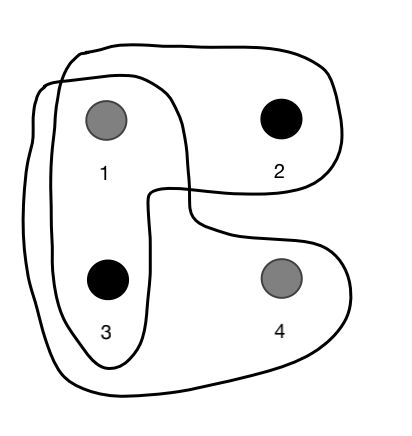
The analysis of properties of hypergraphs, such as their chromatic number, arises when modeling problems in areas as varied as informatics, transportation, molecular biology, and telecommunications, to name just a few (Bretto 2013, see, e.g.,).

Note that $Z$ -tensors with positive minimum $H$ -eigenvalue are strong $M$ -tensors. Thus, computing the minimum $H$ -eigenvalue of $Z$ -tensors is also useful in deciding if a $Z$ -tensor is a strong $M$ -tensor. This question arises when one is interested in finding the sparsest solutions to tensor complementarity problems. Specifically, The authors in (Luo et al. 2017) propose the following optimization problem to find one of the sparsest solutions to a tensor complementarity problem

\text{min:}\ \|x\|_{0},\ \text{s.t.}\ \mathcal{A}x^{m-1}-b\geq 0,\ x\geq 0,\ x^{\intercal}(\mathcal{A}x^{m-1}-b)=0.

(38)

The objective of (38) is written using the nuclear (i.e., $l_{0}$ ) norm. In (Luo et al. 2017), it is shown that if $\mathcal{A}$ is a $Z$ -tensor, then a sparsest solution of the above tensor complementarity problem can be obtained by solving the following polynomial optimization problem

\text{min:}\ \|x\|_{1},\ \text{s.t.}\ \mathcal{A}x^{m-1}=b,\ x\geq 0.

(39)

Furthermore, they show that if $\mathcal{A}$ is a strong $M$ -tensor, problem (39) is uniquely solvable and the unique solution is also an optimal solution to problem (38). Besides, when $\mathcal{A}$ is a strong $M$ -tensor, the authors in (Ding and Wei 2016) propose algorithms which can solve problem (39) in polynomial time. Thus, it is helpful to check if $\mathcal{A}$ in problem (38) is a strong $M$ -tensor so that one can solve it efficiently. In Example 5, we illustrate this result by considering a tensor that is commonly used in the related literature.

Example 5 (Sparse solutions of multilinear systems of equations)

Let $\mathcal{A}$ in (38) be the $Z$ -tensor given by $\mathcal{A}=s\mathcal{I}-\mathcal{D}$ , where $\mathcal{I}\in\mathbb{S}_{3,2}$ is a diagonal tensor and $\mathcal{D}=(d_{i_{1},i_{2},i_{3}})\in\mathbb{S}_{3,2}$ with $d_{i_{1},i_{2},i_{3}}=|\text{tan}(i_{1}+i_{2}+i_{3})|$ . Let $s=(1+\alpha)*\max_{1\leq i\leq 2}(\mathcal{D}{\bf{e}}^{m-1})$ , where ${\bf{e}}$ is vector of ones in dimension $2$ and $a=0.01$ . This example is introduced in (Liang and Dai 2021, Ex. 1). $\mathcal{A}$ is a symmetric tensor, and using (35), we find that $\lambda_{\min}(\mathcal{A})=1.1538$ , which implies that $\mathcal{A}$ is a strong $M$ -tensor. Thus, from (Ding and Wei 2016, Thm. 3.2), if $b$ in (38) is positive, one can solve problem (38) in polynomial time by solving problem (39) and the solution is unique.

Furthermore, Corollary 5 can also be used to obtain lower bounds for the minimum $H$ -eigenvalues of general $M$ -tensors in polynomial time by solving a power cone optimization problem. This follows from the fact that the minimum $H$ -eigenvalues of an $M$ -tensor is always greater than or equal to the minimum $H$ -eigenvalues of its corresponding symmetrized tensor. We prove this fact in the discussion next.

Lemma 4 ((Zhang et al. 2014, Lem. 2.3))

For $m,n\in\mathbb{N}$ and $M$ -tensor $\mathcal{A}\in\mathbb{S}_{m,n}$ ,

\lambda_{\min}(\mathcal{A})={\min}\left\{\mathcal{A}x^{m}:x\in\mathbb{R}^{n},\sum_{i=1}^{n}x_{i}^{m}=1\right\}.

(40)

Let $\tau(\mathcal{A})=\min\{\text{Re}(\lambda):\lambda\in\sigma(\mathcal{A})\}$ where $\sigma(\mathcal{A})$ is the set of all the eigenvalues of $\mathcal{A}$ .

Lemma 5 ((Zhang et al. 2014, Thm. 3.4(a)))

If $m,n\in\mathbb{N}$ and $M$ -tensor $\mathcal{A}\in\mathbb{T}_{m,n}$ , then $\tau(\mathcal{A})$ is an $H$ -eigenvalue of $\mathcal{A}$ . That is $\lambda_{\min}(\mathcal{A})=\tau(\mathcal{A})$ .

In light of Lemma 5, in what follows, we use $\lambda_{\min}(\mathcal{A})$ to refer to $\tau(\mathcal{A})$ for an $M$ -tensor $\mathcal{A}$ .

Lemma 6

If $\mathcal{A}\in\mathbb{T}_{m,n}$ , then

\lambda_{\min}(\mathcal{A})\geq\lambda_{\min}(\text{sym}(\mathcal{A})).

(41)

Proof

From the definition of $H$ -eigenvalue of a tensor (see Section 1), if the real value $\lambda$ is an $H$ -eigenvalue of $\mathcal{A}$ , then there exists $x\in\mathbb{R}^{n}\backslash\{0\}$ such that

\mathcal{A}x^{m-1}=\lambda x^{[m-1]}.

Thus, $\lambda$ satisfies $\mathcal{A}x^{m}=\lambda\sum_{i=1}^{n}x_{i}^{m}$ . When $m$ is even, then clearly $\sum_{i=1}^{n}x_{i}^{m}>0$ . When $m$ is odd, if $\sum_{i=1}^{n}x_{i}^{m}<0$ , one can set $y=-x$ . Then $y$ and $\lambda$ satisfy

\sum_{i=1}^{n}y_{i}^{m}>0,\quad\mathcal{A}y^{m}=\lambda\sum_{i=1}^{n}y_{i}^{m}.

Thus, for each $H$ -eigenvalue $\lambda$ of $\mathcal{A}$ , there exists $x\in\mathbb{R}^{n}\backslash\{0\}$ such that

\sum_{i=1}^{n}x_{i}^{m}>0,\quad\mathcal{A}x^{m}=\lambda\sum_{i=1}^{n}x_{i}^{m}.

Following this result, we have

\lambda\geq{\min}\left\{\mathcal{A}x^{m}:x\in\mathbb{R}^{n},\sum_{i=1}^{n}x_{i}^{m}=1\right\}.

Furthermore, $\lambda\geq\lambda_{\min}(\text{sym}(\mathcal{A}))$ from Lemma 4.

To show the performance of the proposed method in obtaining lower bounds for the minimum $H$ -eigenvalue of general $M$ -tensors, we apply it to compute the lower bounds of the minimum $H$ -eigenvalues of the $M$ -tensors considered in Example 3.1 and Example 3.2 in (Huang et al. 2018) (i.e., different from the tensors in Table 1, here the tensors are directly taken from (Huang et al. 2018)). Namely, in Table 3, we list the best upper and lower bounds for the minimum $H$ -eigenvalue of the $M$ -tensors using the methods proposed in (Huang et al. 2018), versus the lower bounds of the minimum $H$ -eigenvalue of these $M$ -tensors obtained using (35).

			minimum $H$ -eigenvalue
$M$ -tensor			best lower bound	lower bound	best upper bound
	$m$	$n$	(Huang et al. 2018)	(35)	(Huang et al. 2018)
Example 3.1 in (Huang et al. 2018)	3	3	3.0738	4.4404	6.8390
Example 3.2 in (Huang et al. 2018)	3	3	4.0768	6.3122	9.0313

Table 3: Minimum

H

-eigenvalues of asymmetric

M

-tensors.

Table 3 shows that the lower bounds obtained using (35) are much tighter than the lower bounds obtained in (Huang et al. 2018). This empirically indicates that the proposed lower bound is able to provide high quality bounds when comparing with the methods presented in (Huang et al. 2018).

As another application of the results above, one can verify that an asymmetric $Z$ -tensor $\mathcal{A}$ is a strong $M$ -tensor by computing the minimum $H$ -eigenvalue of $\text{sym}(\mathcal{A})$ . From Lemma 6, if $\lambda_{\min}(\text{sym}(\mathcal{A}))>0$ , then $\lambda_{\min}(\mathcal{A})>0$ . Thus, $\mathcal{A}$ is also a strong $M$ -tensor. In Example 6, we use this fact to validate that a tensor that arises when numerical solving a partial differential equation is a strong $M$ -tensor.

Example 6 (Solutions of multilinear systems of equations)

Consider the problem of numerically solving the Klein–Gordon equation (Matsuno 1987; Rheinboldt 1998):

\begin{cases}u(x)^{m-2}\cdot\Delta u(x)=-f(x),&\quad\text{in }\Omega,\\ u(x)=g(x),&\quad\text{on }\partial\Omega,\end{cases}

where $\Delta=\sum_{k=0}^{d}(\partial^{2}/\partial x_{k}^{2})$ , $\Omega=[0,1]^{d}$ , and $m=3,4,\dots$ . When $d=1$ , this Klein–Gordon equation can be discretized as the following multilinear system

\mathcal{L}_{h}x^{m-1}=f,

in which $h=1/(n-1)$ and $\mathcal{L}_{h}=(({\mathcal{L}_{h}})_{i_{1}i_{2},\dots,i_{m}})\in\mathbb{T}_{m,n}$ with entries defined by

\begin{cases}({\mathcal{L}_{h}})_{1,1,\dots,1}=({\mathcal{L}_{h}})_{n,n,\dots,n}=1/h^{2},&\\ ({\mathcal{L}_{h}})_{i,i,\dots,i}=2/h^{2},&\text{for all }i=2,3,\dots,n-1,\\ ({\mathcal{L}_{h}})_{i,i-1,i,\dots,i}=-1/h^{2}(m-1),&\text{for all }i=2,3,\dots,n-1,\\ ({\mathcal{L}_{h}})_{i,i,i-1,\dots,i}=-1/h^{2}(m-1),&\text{for all }i=2,3,\dots,n-1,\\ ({\mathcal{L}_{h}})_{i,i,i,\dots,i-1}=-1/h^{2}(m-1),&\text{for all }i=2,3,\dots,n-1,\\ ({\mathcal{L}_{h}})_{i,i+1,i,\dots,i}=-1/h^{2}(m-1),&\text{for all }i=2,3,\dots,n-1,\\ ({\mathcal{L}_{h}})_{i,i,i+1,\dots,i}=-1/h^{2}(m-1),&\text{for all }i=2,3,\dots,n-1,\\ ({\mathcal{L}_{h}})_{i,i,i,\dots,i+1}=-1/h^{2}(m-1),&\text{for all }i=2,3,\dots,n-1.\end{cases}

When $m=3$ and $n=3$ , with (35), we obtain that $\lambda_{\min}(\text{sym}(\mathcal{L}_{0.5}))=2.6667$ . Thus, using Lemma 6, $\lambda_{\min}(\mathcal{L}_{0.5})\geq\lambda_{\min}(\text{sym}(\mathcal{L}_{0.5}))>0$ . As a result, $\mathcal{L}_{0.5}$ is actually a strong $M$ -tensor and the algorithms in (Ding and Wei 2016; Rheinboldt 1998; Wang et al. 2019b, among others) can be used to solve the discretized multilinear system.

We subsequently explore further applications within the context of high-order Markov chains (Chung 1967).

Example 7 (Application in high-order Markov chains)

The authors in (Li and Ng 2014) introduce an approximated high-order Markov chain model, described as follows.

\mathcal{P}x^{m-1}=x,\quad||x||_{1}=1,

(42)

where $\mathcal{P}=(p_{i_{1}i_{2}\cdots i_{m}})\in\mathbb{T}_{m,n}$ representing an $(m-1)$ th order Markov chain, which is called an $m$ -order $n$ -dimensional transition probability tensor. That is,

p_{i_{1}i_{2}\cdots i_{m}}\geq 0,\quad\sum_{i_{1}\in[n]}p_{i_{1}i_{2}\cdots i_{m}}=1,

(43)

and $x$ is called a vector of random variables with $x_{i}\geq 0$ and $\sum_{i\in[n]}x_{i}=1$ . It was pointed out in (Liu et al. 2018) that the nonlinear system (42) is equivalent to the following equation:

\begin{cases}(\mathcal{I}-\beta\mathcal{P})x^{m-1}=x^{[m-1]}-\beta x,\\ ||x||_{1}=1.\end{cases}

(44)

If we choose the parameter $\beta$ such that $\mathcal{I}-\beta\mathcal{P}$ is a strong $M$ -tensor, then we may use the tensor splitting method proposed in (Liu et al. 2018) to solve the nonlinear equation. We take two examples $\mathcal{P}_{1}$ and $\mathcal{P}_{2}$ in (Liu et al. 2018; Li and Ng 2014); also see (Raftery 1985). The first example $\mathcal{P}_{1}$ pertains to inter-personal relationships, while the second $\mathcal{P}_{2}$ is derived from occupational mobility data for physicists. The two transition probability tensors are defined by

		$\displaystyle\mathcal{P}_{1}(:,:,1)=\begin{pmatrix}0.5810&0.2432&0.1429\\ 0&0.4109&0.0701\\ 0.4190&0.3459&0.7870\end{pmatrix},\mathcal{P}_{1}(:,:,2)=\begin{pmatrix}0.4708&0.1330&0.0327\\ 0.1341&0.5450&0.2042\\ 0.3951&0.3220&0.7631\end{pmatrix},$
		$\displaystyle\mathcal{P}_{1}(:,:,3)=\begin{pmatrix}0.4381&0.1003&0\\ 0.0229&0.4338&0.0930\\ 0.5390&0.4659&0.9070\end{pmatrix}.$

		$\displaystyle\mathcal{P}_{2}(:,:,1)=\begin{pmatrix}0.9000&0.3340&0.3106\\ 0.0690&0.6108&0.0754\\ 0.0310&0.0552&0.6140\end{pmatrix},\mathcal{P}_{2}(:,:,2)=\begin{pmatrix}0.6700&0.1040&0.0805\\ 0.2892&0.8310&0.2956\\ 0.0408&0.0650&0.6239\end{pmatrix},$
		$\displaystyle\mathcal{P}_{2}(:,:,3)=\begin{pmatrix}0.6604&0.0945&0.0710\\ 0.0716&0.6133&0.0780\\ 0.2680&0.2922&0.8501\end{pmatrix}.$

respectively. Their orders $m$ are both 3 and their numbers of states $n$ are both 3. It was pointed out in (Li and Ng 2014) that the model (42) has a unique positive solution for the two transition probability tensors. Using Corollary 5, we find that when $\beta=0.3$ , $\lambda_{\min}(\text{sym}(I-\beta\mathcal{P}_{1}))=0.081666$ and $\lambda_{\min}(\text{sym}(I-\beta\mathcal{P}_{2}))=0.099781$ . Thus, using Lemma 6, $\lambda_{\min}(I-\beta\mathcal{P})\geq\lambda_{\min}(\text{sym}(I-\beta\mathcal{P}))>0$ for $\mathcal{P}=\mathcal{P}_{1}$ and $\mathcal{P}=\mathcal{P}_{2}$ . The tensor splitting method proposed in (Liu et al. 2018) can be utilized to solve the nonlinear equation (44) under these conditions.

5 Minimum $H$ -eigenvalue of the Fan product of symmetric $M$ -tensors

For two tensors $\mathcal{A}=(a_{i_{1}i_{2}\dots i_{m}})\in\mathbb{T}_{m,n}$ and $\mathcal{B}=(b_{i_{1}i_{2}\dots i_{m}})\in\mathbb{T}_{m,n}$ , their Fan product $\mathcal{A}\star\mathcal{B}$ is a tensor defined by

(\mathcal{A}\star\mathcal{B})_{i_{1}i_{2}\dots i_{m}}=(-1)^{\delta_{i_{1}i_{2}\dots i_{m}}+1}a_{i_{1}i_{2}\dots i_{m}}b_{i_{1}i_{2}\dots i_{m}},

(45)

where $\delta_{i_{1}i_{2}\dots i_{m}}=1$ if $i_{1}=i_{2}=\cdots=i_{m}$ , and $\delta_{i_{1}i_{2}\dots i_{m}}=0$ otherwise.

One of the main characteristics of the Fan product is that the Fan product of $M$ -tensors is also an $M$ -tensor (Shen et al. 2019). The authors in (Cheng 2014; Fang 2007; Shen et al. 2019) propose bounds for the minimum $H$ -eigenvalue of $\mathcal{A}\star\mathcal{B}$ where $\mathcal{A}$ and $\mathcal{B}$ are $Z$ -matrices ( $Z$ -tensors). With the help of the proposed new characterisation of symmetric $M$ -tensors, we provide tighter bounds for the minimum $H$ -eigenvalue of the Fan product of symmetric $M$ -tensors. Specifically, we show both theoretically and empirically that our proposed lower bounds are tighter than any of the bounds provided in (Shen et al. 2019).

For a symmetric $M$ -tensor $\mathcal{A}$ , it follows from Theorem 3.3 and 3.4 and Corollary 5 that one can write $\mathcal{A}$ as

\mathcal{A}=\lambda_{\min}(\mathcal{A})\mathcal{I}+\sum_{\vec{i}\in\mathscr{D}_{n}^{m}}\mathcal{A}^{\vec{i}},

(46)

where $\mathcal{A}^{\vec{i}}=(a^{\vec{i}}_{j_{1}j_{2}\dots j_{m}})\in GDD^{+}_{m,n}\cap\mathbb{D}^{{\vec{i}}}_{m,n}$ , for all $\vec{i}\in\mathscr{D}_{n}^{m}$ . Similarly, for another symmetric $M$ -tensor $\mathcal{B}$ , we can also decompose it as

\mathcal{B}=\lambda_{\min}(\mathcal{B})\mathcal{I}+\sum_{\vec{i}\in\mathscr{D}_{n}^{m}}\mathcal{B}^{\vec{i}},

(47)

where $\mathcal{B}^{\vec{i}}=(b^{\vec{i}}_{j_{1}j_{2}\dots j_{m}})\in GDD^{+}_{m,n}\cap\mathbb{D}^{{\vec{i}}}_{m,n}$ , for all $\vec{i}\in\mathscr{D}_{n}^{m}$ . From Theorem 3.5, the decomposition of $\mathcal{A}$ and $\mathcal{B}$ can be done in polynomial time.

Using this decomposition, we obtain tighter lower bounds of the minimum $H$ -eigenvalue for the Fan product of two symmetric $M$ -tensors. Before presenting the lower bounds, we need the following result regarding the minimum $H$ -eigenvalue of $M$ -tensors.

Lemma 7 ((Shen et al. 2019, Lem. 2.2))

If $\mathcal{A}=(a_{i_{1}\dots i_{m}})\in\mathbb{T}_{m,n}$ is an $M$ -tensor, then

\min_{1\leq i\leq n}\frac{(\mathcal{A}x^{m-1})_{i}}{x_{i}^{m-1}}\leq\lambda_{\min}(\mathcal{A})

for any $x=(x_{1},\dots,x_{n})^{\intercal}\in\mathbb{R}^{n}_{++}$ .

For $M$ -tensor $\mathcal{A}=(a_{i_{1}\dots i_{m}})\in\mathbb{S}_{m,n}$ and $\mathcal{B}=(b_{i_{1}\dots i_{m}})\in\mathbb{S}_{m,n}$ and decomposition (46) and (47), let

\displaystyle\Omega_{1}(\mathcal{A},\mathcal{B})=\min_{1\leq i\leq n}\left(a_{ii\dots i}b_{ii\dots i}-\sum_{(i,i_{2},\dots,i_{m})\in\mathscr{D}_{n}^{m}}\frac{1}{\binom{m-1}{\alpha^{\vec{i}}-e_{i}}}{a}_{ii\dots i}^{i,i_{2},\dots,i_{m}}{b}_{ii\dots i}^{i,i_{2},\dots,i_{m}}\right),

(48)

\displaystyle\Omega_{2}(\mathcal{A},\mathcal{B})=\min_{1\leq i\leq n}\left(a_{ii\dots i}b_{ii\dots i}-\sum_{(i,i_{2},\dots,i_{m})\in\mathscr{D}_{n}^{m}}|{a}_{ii_{2}\dots i_{m}}|{b}_{ii\dots i}^{i,i_{2},\dots,i_{m}}\right),

(49)

\displaystyle\Omega_{2}(\mathcal{B},\mathcal{A})=\min_{1\leq i\leq n}\left(a_{ii\dots i}b_{ii\dots i}-\sum_{(i,i_{2},\dots,i_{m})\in\mathscr{D}_{n}^{m}}|{b}_{ii_{2}\dots i_{m}}|{a}_{ii\dots i}^{i,i_{2},\dots,i_{m}}\right),

(50)

and

		$\displaystyle\Omega_{3}(\mathcal{A},\mathcal{B})=\min_{1\leq i\leq n}\bigg(a_{ii\dots i}b_{ii\dots i}-$
		$\displaystyle\qquad\sum_{(i,i_{2},\dots,i_{m})\in\mathscr{D}_{n}^{m}}\big(\|{a}_{ii_{2}\dots i_{m}}\|)^{\frac{1}{2}}(\|{b}_{ii_{2}\dots i_{m}}\|)^{\frac{1}{2}}({a}_{ii\dots i}^{i,i_{2},\dots,i_{m}})^{\frac{1}{2}}({b}_{ii\dots i}^{i,i_{2},\dots,i_{m}})^{\frac{1}{2}}\bigg).$		(51)

Let $\alpha_{i}(\mathcal{A})=\max_{(i_{2},\dots,i_{m})\neq(i,\dots,i)}|a_{ii_{2}\dots i_{m}}|$ for $i\in[n]$ ,

\Gamma_{1}(\mathcal{A},\mathcal{B})=\min_{1\leq i\leq n}\{a_{ii\dots i}\lambda_{\min}(\mathcal{B})+b_{ii\dots i}\lambda_{\min}(\mathcal{A})\}-\lambda_{\min}(\mathcal{A})\lambda_{\min}(\mathcal{B}),

(52)

\Gamma_{2}(\mathcal{A},\mathcal{B})=\min_{1\leq i\leq n}\{a_{ii\dots i}b_{ii\dots i}-\alpha_{i}(\mathcal{A})(b_{ii\dots i}-\lambda_{\min}(\mathcal{B}))\},

(53)

\Gamma_{2}(\mathcal{B},\mathcal{A})=\min_{1\leq i\leq n}\{a_{ii\dots i}b_{ii\dots i}-\alpha_{i}(\mathcal{B})(a_{ii\dots i}-\lambda_{\min}(\mathcal{A}))\},

(54)

and

	$\displaystyle\Gamma_{3}(\mathcal{A},\mathcal{B})$	(55)
$\displaystyle=$	$\displaystyle\min_{1\leq i\leq n}\Bigg\{a_{ii\dots i}b_{ii\dots i}$
	$\displaystyle-(\alpha_{i}(\mathcal{A}))^{\frac{1}{2}}(\alpha_{i}(\mathcal{B}))^{\frac{1}{2}}(a_{ii\dots i}-\lambda_{\min}(\mathcal{A}))^{\frac{1}{2}}(b_{ii\dots i}-\lambda_{\min}(\mathcal{B}))^{\frac{1}{2}}\Bigg\}.$

Expressions (52), (53), (54) and (55) are proposed in (Shen et al. 2019) as lower bounds for the minimum $H$ -eigenvalue of the Fan product of $M$ -tensors. In Theorem 5.1, we prove that the expressions (48), (49), (50) and (51) tighten these lower bounds. As it will be illustrated in Table 4, which of the expression (48), (49), (50) and (51) provides the best lower bound depends on the specific tensors being considered.

Theorem 5.1

For symmetric $M$ -tensors $\mathcal{A}$ and $\mathcal{B}$ ,

(i)

$\Gamma_{1}(\mathcal{A},\mathcal{B})\leq\Omega_{1}(\mathcal{A},\mathcal{B})\leq\lambda_{\min}(\mathcal{A}\star\mathcal{B})$
(ii)

$\Gamma_{2}(\mathcal{A},\mathcal{B})\leq\Omega_{2}(\mathcal{A},\mathcal{B})\leq\lambda_{\min}(\mathcal{A}\star\mathcal{B})$ , $\Gamma_{2}(\mathcal{B},\mathcal{A})\leq\Omega_{2}(\mathcal{B},\mathcal{A})\leq\lambda_{\min}(\mathcal{A}\star\mathcal{B})$
(iii)

$\Gamma_{3}(\mathcal{A},\mathcal{B})\leq\Omega_{3}(\mathcal{A},\mathcal{B})\leq\lambda_{\min}(\mathcal{A}\star\mathcal{B})$

Proof

First, for symmetric $M$ -tensors $\mathcal{A}$ and $\mathcal{B}$ , one can derive the decompositions given in (46) and (47). For each $\vec{i}=(i_{1},i_{2},\dots,i_{m})\in\mathscr{D}_{n}^{m}$ with $\alpha^{\vec{i}}$ as the tight power, since $\mathcal{A}^{\vec{i}}=(a^{\vec{i}}_{j_{1}j_{2}\dots j_{m}})\in GDD^{+}_{m,n}\cap\mathbb{D}^{{\vec{i}}}_{m,n}$ , there exist $u_{i}>0$ for $i\in[n]$ such that

\displaystyle{a}_{ii\cdots i}^{\vec{i}}u_{i}^{m}\geq\binom{m-1}{\alpha^{\vec{i}}-e_{i}}|{a}_{\vec{i}}^{\vec{i}}u_{i_{1}}\cdots u_{i_{m}}|.

(56)

Similarly, there exist $v_{i}>0$ for $i\in[n]$ such that

\displaystyle{b}_{ii\cdots i}^{\vec{i}}v_{i}^{m}\geq\binom{m-1}{\alpha^{\vec{i}}-e_{i}}|{b}_{\vec{i}}^{\vec{i}}v_{i_{1}}\cdots v_{i_{m}}|.

(57)

To show (i), let $z=(z_{1},z_{2},\dots,z_{n})^{\intercal}\in\mathbb{R}^{n}_{++}$ , where $z_{i}=u_{i}v_{i}$ for all $i\in[n]$ . Then for $i\in[n]$ ,

		$\displaystyle\frac{((\mathcal{A}\star\mathcal{B})z^{m-1})_{i}}{z_{i}^{m-1}}$
	$\displaystyle=$	$\displaystyle a_{ii\cdots i}b_{ii\cdots i}-\frac{1}{z_{i}^{m-1}}\left(\sum_{(i_{2},\dots,i_{m})\neq(i,\dots,i)}a_{ii_{2}\dots i_{m}}b_{ii_{2}\dots i_{m}}z_{i_{2}}\cdots z_{i_{m}}\right)$
	$\displaystyle=$	$\displaystyle a_{ii\cdots i}b_{ii\cdots i}-\frac{1}{(u_{i}v_{i})^{m-1}}\sum_{(i_{2},\dots,i_{m})\neq(i,i,\dots,i)}a_{ii_{2}\dots i_{m}}^{i,i_{2},\dots,i_{m}}u_{i_{2}}\cdots u_{i_{m}}b_{ii_{2}\dots i_{m}}^{i,i_{2},\dots,i_{m}}v_{i_{2}}\cdots v_{i_{m}}$
	$\displaystyle\geq$	$\displaystyle a_{ii\cdots i}b_{ii\cdots i}-\left(\sum_{(i,i_{2},\dots,i_{m})\in\mathscr{D}_{n}^{m}}\frac{1}{\binom{m-1}{\alpha^{\vec{i}}-e_{i}}}{a}_{ii\cdots i}^{i,i_{2},\dots,i_{m}}{b}_{ii\cdots i}^{i,i_{2},\dots,i_{m}}\right)$
	$\displaystyle\geq$	$\displaystyle a_{ii\cdots i}b_{ii\cdots i}-\left(\sum_{(i,i_{2},\dots,i_{m})\in\mathscr{D}_{n}^{m}}{a}_{ii\cdots i}^{i,i_{2},\dots,i_{m}}{b}_{ii\cdots i}^{i,i_{2},\dots,i_{m}}\right)$
	$\displaystyle\geq$	$\displaystyle a_{ii\cdots i}b_{ii\cdots i}-\left(\sum_{(i,i_{2},\dots,i_{m})\in\mathscr{D}_{n}^{m}}{a}_{ii\cdots i}^{i,i_{2},\dots,i_{m}}\right)\left(\sum_{(i,i_{2},\dots,i_{m})\in\mathscr{D}_{n}^{m}}{b}_{ii\cdots i}^{i,i_{2},\dots,i_{m}}\right)$
	$\displaystyle=$	$\displaystyle a_{ii\cdots i}b_{ii\cdots i}-(a_{ii\cdots i}-\lambda_{\min}(\mathcal{A}))(b_{ii\cdots i}-\lambda_{\min}(\mathcal{B}))$
	$\displaystyle=$	$\displaystyle a_{ii\dots i}\lambda_{\min}(\mathcal{B})+b_{ii\dots i}\lambda_{\min}(\mathcal{A})-\lambda_{\min}(\mathcal{A})\lambda_{\min}(\mathcal{B}).$

The second to last equality follows from the decompositions (46) and (47). Thus, it follows that

\Gamma_{1}(\mathcal{A},\mathcal{B})\leq\Omega_{1}(\mathcal{A},\mathcal{B})\leq\min_{1\leq i\leq n}\frac{((\mathcal{A}\star\mathcal{B})z^{m-1})_{i}}{z_{i}^{m-1}}\leq\lambda_{\min}(\mathcal{A}\star\mathcal{B}).

To show (ii), let $z=(z_{1},z_{2},\dots,z_{n})^{\intercal}\in\mathbb{R}^{n}_{++}$ , where $z_{i}=u_{i}$ for all $i\in[n]$ . Then for $i\in[n]$ ,

		$\displaystyle\frac{((\mathcal{A}\star\mathcal{B})z^{m-1})_{i}}{z_{i}^{m-1}}$
	$\displaystyle=$	$\displaystyle a_{ii\cdots i}b_{ii\cdots i}-\frac{1}{u_{i}^{m-1}}\left(\sum_{(i_{2},\dots,i_{m})\neq(i,\dots,i)}a_{ii_{2}\dots i_{m}}b_{ii_{2}\dots i_{m}}u_{i_{2}}\cdots u_{i_{m}}\right)$
	$\displaystyle\geq$	$\displaystyle a_{ii\cdots i}b_{ii\cdots i}-\left(\sum_{(i,i_{2},\dots,i_{m})\in\mathscr{D}_{n}^{m}}{a}_{ii\cdots i}^{i,i_{2},\dots,i_{m}}\|b_{ii_{2}\dots i_{m}}\|\right)$
	$\displaystyle\geq$	$\displaystyle a_{ii\cdots i}b_{ii\cdots i}-\alpha_{i}(\mathcal{B})\left(\sum_{(i,i_{2},\dots,i_{m})\in\mathscr{D}_{n}^{m}}{a}_{ii\cdots i}^{i,i_{2},\dots,i_{m}}\right)$
	$\displaystyle=$	$\displaystyle a_{ii\cdots i}b_{ii\cdots i}-\alpha_{i}(\mathcal{B})\left(a_{ii\cdots i}-\lambda_{\min}(\mathcal{A})\right).$

Thus,

\Gamma_{2}(\mathcal{B},\mathcal{A})\leq\Omega_{2}(\mathcal{B},\mathcal{A})\leq\min_{1\leq i\leq n}\frac{((\mathcal{A}\star\mathcal{B})z^{m-1})_{i}}{z_{i}^{m-1}}\leq\lambda_{\min}(\mathcal{A}\star\mathcal{B}).

(58)

Similarly, it then follows that

\Gamma_{2}(\mathcal{A},\mathcal{B})\leq\Omega_{2}(\mathcal{A},\mathcal{B})\leq\min_{1\leq i\leq n}\frac{((\mathcal{A}\star\mathcal{B})z^{m-1})_{i}}{z_{i}^{m-1}}\leq\lambda_{\min}(\mathcal{A}\star\mathcal{B})

by setting $z_{i}=v_{i}$ for all $i\in[n]$ in the proof of (58).

To show (iii), let $z=(z_{1},z_{2},\dots,z_{n})^{\intercal}\in\mathbb{R}^{n}_{++}$ , where $z_{i}=(u_{i})^{\frac{1}{2}}(v_{i})^{\frac{1}{2}}$ for all $i\in[n]$ . Then for $i\in[n]$ ,

		$\displaystyle\frac{((\mathcal{A}\star\mathcal{B})z^{m-1})_{i}}{z_{i}^{m-1}}$
	$\displaystyle=$	$\displaystyle a_{ii\cdots i}b_{ii\cdots i}-\frac{1}{(u_{i}v_{i})^{\frac{m-1}{2}}}\sum_{(i_{2},\dots,i_{m})\neq(i,\dots,i)}a_{ii_{2}\dots i_{m}}u_{i_{2}}^{\frac{1}{2}}\cdots u_{i_{m}}^{\frac{1}{2}}b_{ii_{2}\dots i_{m}}v_{i_{2}}^{\frac{1}{2}}\cdots v_{i_{m}}^{\frac{1}{2}}$
	$\displaystyle\geq$	$\displaystyle a_{ii\cdots i}b_{ii\cdots i}-\sum_{(i,i_{2},\dots,i_{m})\in\mathscr{D}_{n}^{m}}\|a_{ii_{2}\dots i_{m}}\|^{\frac{1}{2}}(a_{ii\cdots i}^{i,i_{2},\dots,i_{m}})^{\frac{1}{2}}\|b_{ii_{2}\dots i_{m}}\|^{\frac{1}{2}}(b_{ii\cdots i}^{i,i_{2},\dots,i_{m}})^{\frac{1}{2}}$
		in what follows, notice that we use $\mathbbm{i}:=(i,i_{2},\cdots,i_{m})$ for ease of presentation
	$\displaystyle\geq$	$\displaystyle a_{ii\cdots i}b_{ii\cdots i}-\left(\sum_{\mathbbm{i}:=(i,i_{2},\dots,i_{m})\in\mathscr{D}_{n}^{m}}\|a_{\mathbbm{i}}\|a_{ii\cdots i}^{\mathbbm{i}}\right)^{\frac{1}{2}}\left(\sum_{\mathbbm{i}:=(i,i_{2},\dots,i_{m})\in\mathscr{D}_{n}^{m}}\|b_{\mathbbm{i}}\|b_{ii\cdots i}^{\mathbbm{i}}\right)^{\frac{1}{2}}$
	$\displaystyle\geq$	$\displaystyle a_{ii\cdots i}b_{ii\cdots i}-\left(\sum_{\mathbbm{i}:=(i,i_{2},\dots,i_{m})\in\mathscr{D}_{n}^{m}}\alpha_{i}(\mathcal{A})a_{ii\cdots i}^{\mathbbm{i}}\right)^{\frac{1}{2}}\left(\sum_{\mathbbm{i}:=(i,i_{2},\dots,i_{m})\in\mathscr{D}_{n}^{m}}\alpha_{i}(\mathcal{B})b_{ii\cdots i}^{\mathbbm{i}}\right)^{\frac{1}{2}}$
	$\displaystyle=$	$\displaystyle a_{ii\cdots i}b_{ii\cdots i}-(\alpha_{i}(\mathcal{A}))^{\frac{1}{2}}(a_{ii\cdots i}-\lambda_{\min}(\mathcal{A}))^{\frac{1}{2}}(\alpha_{i}(\mathcal{B}))^{\frac{1}{2}}(b_{ii\cdots i}-\lambda_{\min}(\mathcal{B}))^{\frac{1}{2}}$
	$\displaystyle=$	$\displaystyle\Gamma_{3}(\mathcal{A},\mathcal{B}).$

The second inequality follows from the Cauchy–Schwarz inequality. Thus,

\Gamma_{3}(\mathcal{A},\mathcal{B})\leq\Omega_{3}(\mathcal{B},\mathcal{A})\leq\min_{1\leq i\leq n}\frac{((\mathcal{A}\star\mathcal{B})z^{m-1})_{i}}{z_{i}^{m-1}}\leq\lambda_{\min}(\mathcal{A}\star\mathcal{B}).

To illustrate how the new bounds introduced in Theorem 5.1 tighten the bounds introduced in (Shen et al. 2019), we compute bounds proposed here (i.e., (48), (49) (50) and (51)) on the minimum $H$ -eigenvalue of the Fan product of the symmetrized tensors in Example 3.9 in (Shen et al. 2019) and compare the results with the bounds (including (52), (53), (54) and (55)) proposed in (Shen et al. 2019).

Example 8

In this example, a tensor $\mathcal{A}=(a_{i_{1}i_{2}i_{3}i_{4}})\in\mathbb{R}^{[4,2]}$ is written in unfolded form as

\displaystyle\mathcal{A}=\left[\begin{array}[]{cc|cc|cc|cc}a_{1111}&a_{1211}&a_{1112}&a_{1212}&a_{1121}&a_{1221}&a_{1122}&a_{1222}\\ a_{2111}&a_{2211}&a_{2112}&a_{2212}&a_{2121}&a_{2221}&a_{2122}&a_{2222}\end{array}\right].

Symmetric $\mathcal{M}$ -tensors $\mathcal{A}_{i}$ , $\mathcal{B}_{i}\in\mathbb{R}^{[4,2]}$ for $i=1,2,3$ are given as follows

\displaystyle\mathcal{A}_{1}=\left[\begin{array}[]{cc|cc|cc|cc}3&-0.5&-0.5&0&-0.5&0&0&-0.25\\ -0.5&0&0&-0.25&0&-0.25&-0.25&2\end{array}\right],

\displaystyle\mathcal{B}_{1}=\left[\begin{array}[]{cc|cc|cc|cc}1.5&-0.125&-0.125&0&-0.125&0&0&-0.625\\ -0.125&0&0&-0.625&0&-0.625&-0.625&2.5\end{array}\right],

\displaystyle\mathcal{A}_{2}=\left[\begin{array}[]{cc|cc|cc|cc}3.8&-0.5&-0.5&-13/30&-0.5&-13/30&-13/30&-0.5\\ -0.5&-13/30&-13/30&-0.5&-13/30&-0.5&-0.5&3.9\end{array}\right],

\displaystyle\mathcal{B}_{2}=\left[\begin{array}[]{cc|cc|cc|cc}3.2&-0.675&-0.675&-1/3&-0.675&-1/3&-1/3&-0.35\\ -0.675&-1/3&-1/3&-0.35&-1/3&-0.35&-0.35&3.9\end{array}\right],

\displaystyle\mathcal{A}_{3}=\left[\begin{array}[]{cc|cc|cc|cc}3.8&-0.575&-0.575&-11/30&-0.575&-11/30&-11/30&-0.4\\ -0.575&-11/30&-11/30&-0.4&-11/30&-0.4&-0.4&3.7\end{array}\right],

\displaystyle\mathcal{B}_{3}=\left[\begin{array}[]{cc|cc|cc|cc}3.5&-0.35&-0.35&-23/60&-0.35&-23/60&-23/60&-0.525\\ -0.35&-23/60&-23/60&-0.525&-23/60&-0.525&-0.525&3.1\end{array}\right],

Similar to Table 1 in (Shen et al. 2019), Table 4 shows the bounds for the minimum $H$ -eigenvalue of the Fan product of $\mathcal{A}_{i}$ and $\mathcal{B}_{i}$ , $i=1,2,3$ obtained with the expressions (48), (49), (50), (51) and the lower bound expressions from (Shen et al. 2019). For $\mathcal{A}_{i}$ and $\mathcal{B}_{i}$ , $i=1,2,3$ , the lower bounds from (48) are 4.0717, 10.8346 and 10.3187 respectively which are larger than the values from all the bounds proposed in (Shen et al. 2019). Besides, the lower bounds from (49), (50) and (51) are also tighter than the lower bounds from (3.4), (3.5) and (3.6) (i.e., (53), (54), and(55)) in (Shen et al. 2019), respectively. This empirically validates the fact that the proposed bounds (48), (49), (50), (51) are tighter lower bounds for the minimum $H$ -eigenvalue of the Fan product of two symmetric $M$ -tensors. The proposed bounds (48), (49), (50) and (51) contain more information comparing the bounds proposed in (Shen et al. 2019). As a result, they are able to provide the tighter lower bounds. Note also that the expression among (48), (49), (50) and (51) that provides the best lower bound depends on the specific tensors. For example in the first column ( $\mathcal{A}_{1}$ and $\mathcal{B}_{1}$ ), the best lower bound is given by expression (49) while for the second column ( $\mathcal{A}_{2}$ and $\mathcal{B}_{2}$ ) it is expression (48).

	$\mathcal{A}=\mathcal{A}_{1},\mathcal{B}=\mathcal{B}_{1}$	$\mathcal{A}=\mathcal{A}_{2},\mathcal{B}=\mathcal{B}_{2}$	$\mathcal{A}=\mathcal{A}_{3},\mathcal{B}=\mathcal{B}_{3}$
$\lambda_{\min}(\mathcal{A})$	0.9723	0.54995	0.6970
$\lambda_{\min}(\mathcal{B})$	0.5000	0.41253	0.3717
$\lambda_{\min}(\mathcal{A}\star\mathcal{B})$	4.2762	11.3818	12.0646
Lower bounds on $\lambda_{\min}(\mathcal{A}\star\mathcal{B})$ from (Shen et al. 2019)
(3.1) in (Shen et al. 2019)	2.4722	3.1006	3.2768
(3.3) in (Shen et al. 2019) (52)	4.0000	10.7663	9.9012
(3.4) in (Shen et al. 2019) (53)	3.2327	9.9662	9.8934
(3.5) in (Shen et al. 2019) (54)	4.0000	10.7663	9.9012
(3.6) in (Shen et al. 2019) (55)	3.7040	10.4114	9.8973
(3.7) in (Shen et al. 2019)	2.5000	10.2250	2.6294
Proposed lower bounds on $\lambda_{\min}(\mathcal{A}\star\mathcal{B})$
(48)	4.0717	10.8346	10.3187
(49)	4.1562	10.8177	10.3682
(50)	4.0717	10.5605	10.1657
(51)	4.1169	10.6959	10.2691

Table 4: Lower bounds for the minimum

H

-eigenvalues of the Fan product of symmetric

M

-tensors.

6 Conclusions

In this work, a new characterization of symmetric $H^{+}$ -tensors is presented (see Corollary (2)). As a result of this characterization, it follows that one can identify whether a tensor is a symmetric $H^{+}$ -tensor in polynomial time (see Theorem 3.5). Comparing other characterizations which typically focus on sufficient conditions for a tensor to be an $H^{+}$ -tensor, our characterization provides sufficient and necessary conditions. Besides, the set of symmetric $H^{+}$ -tensors is described using tractable convex cones; in particular, the power cone.

We apply the new characterization of symmetric $H^{+}$ -tensors in computing the minimum $H$ -eigenvalue of symmetric $M$ -tensors. In particular, we compare the best bounds for the minimum $H$ -eigenvalues proposed in the related literature with these $H$ -eigenvalues of symmetric $M$ -tensors; which can be computed in polynomial time by solving a power cone optimization problem. We also show that this approach to computing $H$ -eigenvalues of symmetric $M$ -tensors is more efficient than using homotopy continuation type algorithms that allow the more general computation of complex generalized tensor eigenpairs (Chen et al. 2016b). Furthermore, we illustrate how this new characterization of symmetric $H^{+}$ -tensors can be used to obtain tighter lower bounds for the minimum $H$ -eigenvalue of the Fan product of two symmetric $M$ -tensors. We show both theoretically and empirically that the proposed bounds are tighter compared to the bounds proposed in (Shen et al. 2019). We illustrate the relevance of our results with practical examples drawn from polynomial optimization, hypergraphs analysis, complementarity problems, multilinear systems, and high-order Markov chains. Besides these applications, we believe more interesting results can be obtained with the proposed new characterization of symmetric $H^{+}$ -tensors and $M$ -tensors.

References

Ahmadi and Majumdar (2019) Amir Ali Ahmadi and Anirudha Majumdar. DSOS and SDSOS optimization: more tractable alternatives to sum of squares and semidefinite optimization. SIAM Journal on Applied Algebra and Geometry, 3(2):193–230, 2019.
ApS (2022) MOSEK ApS. MOSEK optimization suite, 2022. URL https://docs.mosek.com/9.3/releasenotes/index.html#.
ApS (2024) MOSEK ApS. MOSEK Modeling Cookbook, 2024. URL https://docs.mosek.com/modeling-cookbook/powo.html.
Azimzadeh and Bayraktar (2019) Parsiad Azimzadeh and Erhan Bayraktar. High order bellman equations and weakly chained diagonally dominant tensors. SIAM Journal on Matrix Analysis and Applications, 40(1):276–298, 2019.
Bader et al. (2019) Brett W. Bader, Tamara G. Kolda, et al. Tensor toolbox for MATLAB, version 3.1. www.tensortoolbox.org, June 2019. Accessed June 4, 2019.
Boman et al. (2005) Erik G Boman, Doron Chen, Ojas Parekh, and Sivan Toledo. On factor width and symmetric $H$ -matrices. Linear Algebra and its Applications, 405:239–248, 2005.
Bretto (2013) Alain Bretto. Applications of hypergraph theory: a brief overview. Hypergraph Theory, pages 111–116, 2013.
Cartwright and Sturmfels (2013) Dustin Cartwright and Bernd Sturmfels. The number of eigenvalues of a tensor. Linear Algebra and its Applications, 438(2):942–952, 2013.
Chang et al. (2013) Kungching Chang, Liqun Qi, and Tan Zhang. A survey on the spectral theory of nonnegative tensors. Numerical Linear Algebra with Applications, 20(6):891–912, 2013.
Chares (2009) Robert Chares. Cones and interior-point algorithms for structured convex optimization involving powers and exponentials. PhD thesis, UCL-Université Catholique de Louvain, Louvain-la-Neuve, Belgium, 2009.
Chen et al. (2016a) Haibin Chen, Guoyin Li, and Liqun Qi. SOS tensor decomposition: Theory and applications. Communications in Mathematical Sciences, 14(8):2073–2100, 2016a.
Chen et al. (2016b) Liping Chen, Lixing Han, and Liangmin Zhou. Computing tensor eigenvalues via homotopy methods. SIAM Journal on Matrix Analysis and Applications, 37(1):290–319, 2016b.
Chen and Goulart (2023) Yuwen Chen and Paul Goulart. An efficient IPM implementation for a class of nonsymmetric cones. arXiv preprint arXiv:2305.12275, 2023.
Chen et al. (2024) Yuwen Chen, Danny Tse, Parth Nobel, Paul Goulart, and Stephen Boyd. CuClarabel: GPU acceleration for a conic optimization solver. arXiv preprint arXiv:2412.19027, 2024.
Cheng (2014) Guanghui Cheng. New bounds for the minimum eigenvalue of the Fan product of two $M$ -matrices. Czechoslovak Mathematical Journal, 64(1):63–68, 2014.
Chung (1967) Kai Lai Chung. Markov chains. Springer-Verlag, New York, 1967.
Coey et al. (2022) Chris Coey, Lea Kapelevich, and Juan Pablo Vielma. Solving natural conic formulations with Hypatia.jl. INFORMS Journal on Computing, 34(5):2686–2699, 2022.
Cooper and Dutle (2012) Joshua Cooper and Aaron Dutle. Spectra of uniform hypergraphs. Linear Algebra and its Applications, 436(9):3268–3292, 2012.
Ding and Wei (2016) Weiyang Ding and Yimin Wei. Solving multi-linear systems with $M$ -tensors. Journal of Scientific Computing, 68(2):689–715, 2016.
Ding et al. (2013) Weiyang Ding, Liqun Qi, and Yimin Wei. $M$ -tensors and nonsingular $M$ -tensors. Linear Algebra and its Applications, 439(10):3264–3278, 2013.
Fan (1964) Ky Fan. Inequalities for $M$ -matrices. Indag. Math, 26:602–610, 1964.
Fan et al. (2019) Yi-Zheng Fan, Yi Wang, and Yan-Hong Bao. Eigenvectors of $Z$ -tensors associated with least $H$ -eigenvalue with application to hypergraphs. arXiv preprint arXiv:1901.08222, 2019.
Fang (2007) Maozhong Fang. Bounds on eigenvalues of the Hadamard product and the Fan product of matrices. Linear Algebra and its Applications, 425(1):7–15, 2007.
Friberg (2024) Henrik A. Friberg. An exponential cone representation of the general power cone. Technical report, Optimization Online, 2024. Available at https://optimization-online.org/?p=26665.
Galuppi et al. (2023) Francesco Galuppi, Raffaella Mulas, and Lorenzo Venturello. Spectral theory of weighted hypergraphs via tensors. Linear and Multilinear Algebra, 71(3):317–347, 2023.
Goulart and Chen (2024) Paul J. Goulart and Yuwen Chen. Clarabel: An interior-point solver for conic programs with quadratic objectives, 2024.
Han (2017) Lixing Han. A homotopy method for solving multilinear systems with $M$ -tensors. Applied Mathematics Letters, 69:49–54, 2017.
He and Huang (2014) Jun He and Ting-Zhu Huang. Inequalities for $M$ -tensors. Journal of Inequalities and Applications, 2014(1):114, 2014.
Hien (2015) Le Thi Khanh Hien. Differential properties of Euclidean projection onto power cone. Mathematical Methods of Operations Research, 82:265–284, 2015.
Hillar and Lim (2013) Christopher J Hillar and Lek-Heng Lim. Most tensor problems are NP-hard. Journal of the ACM (JACM), 60(6):1–39, 2013.
Huang and Ma (2019a) Baohua Huang and Changfeng Ma. Iterative criteria for identifying strong $H$ -tensors. Journal of Computational and Applied Mathematics, 352:93–109, 2019a.
Huang and Ma (2019b) Baohua Huang and Changfeng Ma. Some criteria for identifying strong $H$ -tensors and its applications. Linear and Multilinear Algebra, 67(6):1146–1173, 2019b.
Huang et al. (2018) Zheng-Ge Huang, Li-Gong Wang, Zhong Xu, and Jing-Jing Cui. Some new inequalities for the minimum $H$ -eigenvalue of nonsingular $M$ -tensors. Linear Algebra and its Applications, 558:146–173, 2018.
Huang and Qi (2017) Zheng-Hai Huang and Liqun Qi. Formulating an $n$ -person noncooperative game as a tensor complementarity problem. Computational Optimization and Applications, 66:557–576, 2017.
Jos (2025) Jos. allcomb(varargin). MATLAB Central File Exchange, 2025. URL https://www.mathworks.com/matlabcentral/fileexchange/10064-allcomb-varargin. Retrieved February 1, 2025.
Kannan et al. (2015) M Rajesh Kannan, Naomi Shaked-Monderer, and Abraham Berman. Some properties of strong $H$ -tensors and general $H$ -tensors. Linear Algebra and its Applications, 476:42–55, 2015.
Karimi and Tunçel (2024) Mehdi Karimi and Levent Tunçel. Domain-Driven Solver (DDS) version 2.1: a MATLAB-based software package for convex optimization problems in domain-driven form. Mathematical Programming Computation, 16(1):37–92, 2024.
Koecher (1957) Max Koecher. Positivitätsbereiche im $\mathbb{R}^{n}$ . American Journal of Mathematics, 79(3):575–596, 1957.
Kuryatnikova et al. (2024) Olga Kuryatnikova, Juan C Vera, and Luis F Zuluaga. Reducing nonnegativity over general semialgebraic sets to nonnegativity over simple sets. SIAM Journal on Optimization, 34(2):1970–2006, 2024.
Landsberg (2012) Joseph M Landsberg. Tensors: geometry and applications. Representation Theory, 381(402):3, 2012.
Lasserre (2015) Jean Bernard Lasserre. An introduction to polynomial and semi-algebraic optimization, volume 52. Cambridge University Press, 2015.
Li et al. (2013) Chaoqian Li, Yaotang Li, and Ruijuan Zhao. New inequalities for the minimum eigenvalue of $M$ -matrices. Linear and Multilinear Algebra, 61(9):1267–1279, 2013.
Li et al. (2014) Chaoqian Li, Feng Wang, Jianxing Zhao, Yan Zhu, and Yaotang Li. Criterions for the positive definiteness of real supersymmetric tensors. Journal of Computational and Applied Mathematics, 255:1–14, 2014.
Li and Ng (2014) Wen Li and Michael K Ng. On the limiting probability distribution of a transition probability tensor. Linear and Multilinear Algebra, 62(3):362–385, 2014.
Li and Ng (2015) Xutao Li and Michael K Ng. Solving sparse non-negative tensor equations: algorithms and applications. Frontiers of Mathematics in China, 10:649–680, 2015.
Li et al. (2017) Yaotang Li, Qilong Liu, and Liqun Qi. Programmable criteria for strong $H$ -tensors. Numerical Algorithms, 74(1):199–221, 2017.
Liang and Dai (2021) Maolin Liang and Lifang Dai. Alternating minimization methods for solving multilinear systems. Mathematical Problems in Engineering, 2021, 2021.
Lim (2005) Lek-Heng Lim. Singular values and eigenvalues of tensors: a variational approach. In 1st IEEE International Workshop on Computational Advances in Multi-Sensor Adaptive Processing, 2005., pages 129–132. IEEE, 2005.
Liu et al. (2018) Dongdong Liu, Wen Li, and Seak-Weng Vong. The tensor splitting with application to solve multi-linear systems. Journal of Computational and Applied Mathematics, 330:75–94, 2018.
Liu et al. (2017) Qilong Liu, Chaoqian Li, and Yaotang Li. On the iterative criterion for strong $H$ -tensors. Computational and Applied Mathematics, 36(4):1623–1635, 2017.
Liu et al. (2020) Qilong Liu, Jianxing Zhao, Chaoqian Li, and Yaotang Li. An iterative algorithm based on strong $H$ -tensors for identifying positive definiteness of irreducible homogeneous polynomial forms. Journal of Computational and Applied Mathematics, 369:112581, 2020.
Lobo et al. (1998) Miguel Sousa Lobo, Lieven Vandenberghe, Stephen Boyd, and Hervé Lebret. Applications of second-order cone programming. Linear Algebra and its Applications, 284(1-3):193–228, 1998.
Luan and Zhang (2019) Zhenting Luan and Liping Zhang. A new programmable iterative algorithm for identifying strong $H$ -tensors. Computational and Applied Mathematics, 38(2):43, 2019.
Luo and Qi (2015) Ziyan Luo and Liqun Qi. Doubly nonnegative tensors, completely positive tensors and applications. arXiv preprint arXiv:1504.07806, 2015.
Luo and Qi (2016) Ziyan Luo and Liqun Qi. Completely positive tensors: properties, easily checkable subclasses, and tractable relaxations. SIAM Journal on Matrix Analysis and Applications, 37(4):1675–1698, 2016.
Luo et al. (2015) ZiYan Luo, LiQun Qi, and YinYu Ye. Linear operators and positive semidefiniteness of symmetric tensor spaces. Science China Mathematics, 58(1):197–212, 2015.
Luo et al. (2017) Ziyan Luo, Liqun Qi, and Naihua Xiu. The sparsest solutions to $Z$ -tensor complementarity problems. Optimization Letters, 11(3):471–482, 2017.
Matsuno (1987) Y Matsuno. Exact solutions for the nonlinear Klein-Gordon and Liouville equations in four-dimensional Euclidean space. Journal of mathematical physics, 28(10):2317–2322, 1987.
Megretski (2010) A. Megretski. Systems Polynomial Optimization Tools (SPOT). https://github.com/spot-toolbox/spotless, 2010.
Nesterov (2012) Yurii Nesterov. Towards non-symmetric conic optimization. Optimization Methods and Software, 27(4-5):893–917, 2012.
O’Donoghue et al. (2016) Brendan O’Donoghue, Eric Chu, Neal Parikh, and Stephen Boyd. Conic optimization via operator splitting and homogeneous self-dual embedding. Journal of Optimization Theory and Applications, 169(3):1042–1068, June 2016. URL http://stanford.edu/~boyd/papers/scs.html.
Papp and Yıldız (2022) Dávid Papp and Sercan Yıldız. alfonso: Matlab package for nonsymmetric conic optimization. INFORMS Journal on Computing, 34(1):11–19, 2022.
Qi (2005) Liqun Qi. Eigenvalues of a real supersymmetric tensor. Journal of Symbolic Computation, 40(6):1302–1324, 2005.
Qi (2013) Liqun Qi. Symmetric nonnegative tensors and copositive tensors. Linear Algebra and its Applications, 439(1):228–238, 2013.
Qi (2014) Liqun Qi. ${H}^{+}$ -eigenvalues of Laplacian and signless Laplacian tensors. Communications in Mathematical Sciences, 12(6):1045–1064, 2014.
Raftery (1985) Adrian E Raftery. A model for high-order Markov chains. Journal of the Royal Statistical Society Series B: Statistical Methodology, 47(3):528–539, 1985.
Renegar (2001) James Renegar. A mathematical view of interior-point methods in convex optimization, volume 3. SIAM, 2001.
Rheinboldt (1998) Werner C Rheinboldt. Methods for solving systems of nonlinear equations. SIAM, 1998.
Roy and Xiao (2022) Scott Roy and Lin Xiao. On self-concordant barriers for generalized power cones. Optimization Letters, 16(2):681–694, 2022.
Shen et al. (2019) Jihong Shen, Yue Wang, and Changjiang Bu. Some inequalities on the minimum $H$ -eigenvalue of the Fan product of $Z$ -tensors. Linear Algebra and its Applications, 579:55–71, 2019.
Sun (2020) Deshu Sun. New methods based on $H$ -tensors for identifying positive definiteness of homogeneous polynomial forms. Linear and Multilinear Algebra, 68(12):2473–2483, 2020.
Sun et al. (2019) Lizhu Sun, Jiang Zhou, and Changjiang Bu. Spectral properties of general hypergraphs. Linear Algebra and its Applications, 561:187–203, 2019.
Tian and Huang (2010) Gui-Xian Tian and Ting-Zhu Huang. Inequalities for the minimum eigenvalue of $M$ -matrices. The Electronic Journal of Linear Algebra, 20, 2010.
Tunçel and Nemirovski (2010) Levent Tunçel and Arkadi Nemirovski. Self-concordant barriers for convex approximations of structured convex sets. Foundations of Computational Mathematics, 10(5):485–525, 2010.
Varga and Gillis (1963) Richard S Varga and J Gillis. Matrix iterative analysis. Physics Today, 16:52, 1963.
Wang et al. (2017) Feng Wang, Deshu Sun, Jianxing Zhao, and Chaoqian Li. New practical criteria for $H$ -tensors and its application. Linear and Multilinear Algebra, 65(2):269–283, 2017.
Wang et al. (2019a) Xuezhong Wang, Maolin Che, and Yimin Wei. Existence and uniqueness of positive solution for $H^{+}$ -tensor equations. Applied Mathematics Letters, 98:191–198, 2019a.
Wang et al. (2019b) Xuezhong Wang, Maolin Che, and Yimin Wei. Neural networks based approach solving multi-linear systems with $M$ -tensors. Neurocomputing, 351:33–42, 2019b.
Wang et al. (2020a) Xuezhong Wang, Maolin Che, and Yimin Wei. Global uniqueness and solvability of tensor complementarity problems for $H_{+}$ -tensors. Numerical Algorithms, 84(2):567–590, 2020a.
Wang et al. (2020b) Xuezhong Wang, Maolin Che, and Yimin Wei. Preconditioned tensor splitting aor iterative methods for $H$ -tensor equations. Numerical Linear Algebra with Applications, 27(6):e2329, 2020b.
Wang et al. (2021) Xuezhong Wang, Changxin Mo, Maolin Che, and Yimin Wei. Accelerated dynamical approaches for finding the unique positive solution of KS-tensor equations. Numerical Algorithms, 88(4):1787–1810, 2021.
Wright (1997) Stephen J Wright. Primal-dual interior-point methods. SIAM, 1997.
Zhang et al. (2016) Hongliang Zhang, Lingyang Song, and Zhu Han. Radio resource allocation for device-to-device underlay communication using hypergraph theory. IEEE Transactions on Wireless Communications, 15(7):4852–4861, 2016.
Zhang and Wang (2016) Kaili Zhang and Yiju Wang. An $H$ -tensor based iterative scheme for identifying the positive definiteness of multivariate homogeneous forms. Journal of Computational and Applied Mathematics, 305:1–10, 2016.
Zhang et al. (2012) Liping Zhang, Liqun Qi, and Guanglu Zhou. $M$ -tensors and the positive definiteness of a multivariate form. arXiv preprint arXiv:1202.6431, 2012.
Zhang et al. (2014) Liping Zhang, Liqun Qi, and Guanglu Zhou. $M$ -tensors and some applications. SIAM Journal on Matrix Analysis and Applications, 35(2):437–452, 2014.
Zhao et al. (2016) Ruijuan Zhao, Lei Gao, Qilong Liu, and Yaotang Li. Criterions for identifying $H$ -tensors. Frontiers of Mathematics in China, 11(3):661–678, 2016.

A new characterization of symmetric H+H^{+}-tensors and MM-tensors Thanks: This research did not receive any specific grant from funding agencies in the public, commercial, or not-for-profit sectors.

Abstract

Keywords:

MSC

1 Introduction

2 Preliminaries

Theorem 2.1 ((Chen et al. 2016a, Thm. 3.7))

Definition 1 ((Luo and Qi 2016, Def. 6.5))

Proposition 1

Proof

Theorem 2.2 ((Kannan et al. 2015, Thm. 4.9))

Corollary 1

Definition 2

Example 1

3 New characterization of symmetric H+H^{+}-tensors

Proposition 2

Proof

Theorem 3.1 ((Qi 2013, Thm. 1(a)))

Theorem 3.2 ((Qi 2013, Thm. 2))

Proposition 3

Proof

Proposition 4 ((Kannan et al. 2015, Prop. 2.7))

Proposition 5

Proof

Theorem 3.3

Proof

Lemma 1 ((Ahmadi and Majumdar 2019, Lem. 3.8))

Theorem 3.4

Proof

Corollary 2

Proof

Example 2

3.1 Identifying symmetric H+H^{+}-tensors with power cone optimization

Definition 3 (High-dimensional power cone (Chares 2009, Sec. 4.1.2))

Corollary 3

Theorem 3.5

Proof

Definition 4

Example 3 (Application in polynomial optimization)

4 Minimum HH-eigenvalue of MM-tensors

Lemma 2 ((Zhang et al. 2014, Lem. 2.2))

Lemma 3

Proof

Proposition 6

Proof

Corollary 4

Corollary 5

Proof

Definition 5 ((Chang et al. 2013, Def. 6.1))

Definition 6 ((Chang et al. 2013, Def. 6.2))

Theorem 4.1 ((Cooper and Dutle 2012, Thm. 3.10))

Example 4 (Hypergraph application)

Example 5 (Sparse solutions of multilinear systems of equations)

Lemma 4 ((Zhang et al. 2014, Lem. 2.3))

Lemma 5 ((Zhang et al. 2014, Thm. 3.4(a)))

Lemma 6

Proof

Example 6 (Solutions of multilinear systems of equations)

Example 7 (Application in high-order Markov chains)

5 Minimum HH-eigenvalue of the Fan product of symmetric MM-tensors

Lemma 7 ((Shen et al. 2019, Lem. 2.2))

Theorem 5.1

Proof

Example 8

6 Conclusions

References

A new characterization of symmetric $H^{+}$ -tensors and $M$ -tensors Thanks: This research did not receive any specific grant from funding agencies in the public, commercial, or not-for-profit sectors.

3 New characterization of symmetric $H^{+}$ -tensors

3.1 Identifying symmetric $H^{+}$ -tensors with power cone optimization

4 Minimum $H$ -eigenvalue of $M$ -tensors

5 Minimum $H$ -eigenvalue of the Fan product of symmetric $M$ -tensors