跳到论文正文
W Papers独立论文阅读器 arXiv:2008.08082 论文正文 计算阅读时间 · 0%
引用这篇论文根据当前论文元数据生成,正式投稿前建议核对。


License: arXiv.org perpetual non-exclusive license
arXiv:2008.08082v1 [math.CA] 18 Aug 2020

УДК 517.9

MSC 26A33, 74S40

Fractional powers of Bessel operator and its numerical calculation

Durdimurod K. Durdiev
Bukhara Branch of the Institute of Mathematics at the Academy of Sciences of the Republic of Uzbekistan, Bukhara, Uzbekistan

durdiev65@mail.ru

Elina L. Shishkina
Voronezh State University, Voronezh, Russia

shishkina@amm.vsu.ru

Sergei M. Sitnik
Belgorod State University, Belgorod, Russia

sitnik@bsu.edu.ru

Дурдимурод Каландарович Дурдиев

Бухарское отделение института Математики АН РУз, Бухара, Узбекистан

durdiev65@mail.ru

Шишкина Элина Леонидовна

Воронежский государственный университет, Воронеж, Россия

shishkina@amm.vsu.ru

Ситник Сергей Михайлович

Белгородский государственный национальный исследовательский университет, Белгород, Россия

sitnik@bsu.edu.ru

Keywords: Bessel operator, fractional powers, Hankel integral transforms, composition method, transmutation operators

Ключевые слова: оператор Бесселя, дробные степени, преобразование Ханкеля, обобщённый сдвиг, композиционный метод, операторы преобразования

Abstract. The article discusses the fractional powers of the Bessel operator and their numerical implementation. An extensive literature is devoted to the study of fractional powers of the Laplace operator and their applications. Such degrees are used in the construction of functional spaces, in the natural generalization of the Schrödinger equation in quantum theory, in the construction of the models of acoustic wave propagation in complex media (for example, biological tissues) and space-time models of anomalous (very slow or very fast) diffusion, in spectral theory etc. If we assume the radiality of the function on which the Laplace operator acts, then we receive the problem of constructing the fractional power of the Bessel operator. We propose to use a compositional method for constructing the operators mentioned earlier, which leads to constructions similar in their properties to the Riesz derivatives. The Hankel transform is considered as a basic integral transformation. On its basis, the compositional method proposed by V.V. Katrakhov and S.M. Sitnik, negative powers of the Bessel operator are constructed. The resulting operator contains the Gaussian hypergeometric function in the kernel. For further study, the generalized translation operator is considered in the article, and its properties are proved. For constructing a positive fractional power of the Bessel operator known methods of regularization of the integral are considered. Then, a scheme for the numerical calculation of fractional powers of the Bessel operator is proposed. This scheme is based on the Taylor–Delsarte formula obtained by B.M. Levitan. Examples containing the exact and approximate values of the positive and negative powers of the Bessel operator, the absolute error, and illustrations are given. The list of references contains sources with known results on similar fractional operators, as well as applications of them.

Аннотация. В статье рассматриваются дробные степени оператора Бесселя и их численная реализация. Обширная литература посвящена изучению дробных степеней оператора Лапласа и их приложениям. Такие степени используются при конструировании функциональных пространств, при естественном обобщении уравнения Шрёдингера в квантовой теории, при построении моделей распространения акустических волн в сложных средах (например, биологических тканях) и пространственно-временных моделей аномальной (очень медленной или очень быстрой) диффузии, в спектральной теории и др. Если предположить радиальность функции, на которую действует оператор Лапласа, то мы придем к задаче о построении дробной степени оператора Бесселя. Мы предлагаем использовать композиционный метод построения указанных операторов, что приводит к конструкциям, близким по своим свойствам к Риссовым производным. В качестве базового интегрального преобразования рассматривается преобразование Ханкеля. На его основе композиционным методом, предложенным В. В. Катраховым и С.М. Ситником, строятся отрицательные степени оператора Бесселя. Полученный оператор содержит в ядре гипергеометрическую функцию Гаусса. Для дальнейшего изучения в статье приводится оператор обобщенного сдвига, доказываются его свойства. Известными способами достигается регуляризация интеграла при построении положительной дробной степени оператора Бесселя. Затем предлагается схема численного вычисления дробных степеней оператора Бесселя, основанная на полученной Б.М. Левитаном формуле Тейлора–Дельсарта. Приводятся примеры, содержащие точное и приближенное значения положительной и отрицательной степеней оператора Бесселя, абсолютную погрешность и иллюстрации. В списке литературы приводятся источники, в которых содержатся известные результаты о дробных степенях операторов, рассматриваемого в статье типа, а также содержащие их приложения.

1 Introduction

We will consider fractional powers (Bγ)α({B}_{\gamma})^{\alpha}, α∈ℝ\alpha\in\mathbb{R} of differential Bessel operator in the form

Bγ=D2+γx​D,γ≥0,D:=dd​x.B_{\gamma}=D^{2}+\frac{\gamma}{x}D,\qquad\gamma\geq 0,\ \ \ D:=\frac{d}{dx}. (1)

This fractional power will be constructed using Integral Transforms Composition Method (ITCM) [1, 2, 3]. For more detailed discussion of the fractional powers of (1) on a segment and an semi-axes we refer to [4, 5]. Negative fractional degrees of the operator (1) obtained in this way are one-dimensional Riesz B-potentials studied in [6, 7, 8, 9, 10].

The potential theory comes from mathematical physics. The most well-known areas of its application are electrostatic and gravitational theory, probability theory, scattering theory, biological systems and other.

First application of classical Riesz potentials was given by M. Riesz himself and it was a solution of Maxwell’s equations for the electromagnetic field (see [11], p. 146, and [12]). Maxwell’s equations are fundamental equations of the classical electrodynamics and optics. The equations completely describe all electromagnetic phenomena in an arbitrary environment and provide a mathematical model for electric, optical and radio technologies, such as power generation, electric motors, wireless communication, lenses, radar etc. So Riesz potentials can be used for studying of realistic single particle energy levels.

An interesting fact was noticed in [13]. Namely, in this paper it was shown that Riesz potential can be interpreted as a transmutation operator. More precisely, the operator square root of the Laplacian was obtained from the harmonic extension problem to the upper half space as the operator that maps the Dirichlet boundary condition to the Neumann condition. The same result but for hyperbolic Riesz potentials was obtained in [14].

2 Construction of fractional power of Bessel operator by ITCM

In this section using integral transform composition method we construct the operator 𝐈γα\mathbf{I}^{\alpha}_{\gamma} which is the negative fractional power of Bessel operator: (Bγ)α=𝐈γα(B_{\gamma})^{\alpha}=\mathbf{I}^{\alpha}_{\gamma}, α>0\alpha>0. To do this, we use a suitable integral transformation it is the Hankel transform.

Let γ>0\gamma>0. The one-dimentional Hankel transform of a function ff, such that f⁡(x)​xγ∈L1​(0,∞)f(x)x^{\gamma}{\in}L_{1}(0,\infty) is expressed as

Hγ​[f]​(ξ)=Hγ​[f⁡(x)]​(ξ)=f⁡(ξ)=∫0∞f⁡(x)​jγ−12​(x​ξ)​xγ​𝑑x,{H}_{\gamma}[f](\xi)={H}_{\gamma}[f(x)](\xi)={f}(\xi)=\int\limits_{0}^{\infty}f(x)\,{j}_{\frac{\gamma-1}{2}}(x\xi)x^{\gamma}dx, (2)

where the symbol jνj_{\nu} is used for the normalized Bessel function of the first kind (see [15], p. 10, [16]):

jν​(x)=2ν​Γ​(ν+1)xν​Jν​(x),j_{\nu}(x)=\frac{2^{\nu}\Gamma(\nu+1)}{x^{\nu}}\,\,J_{\nu}(x), (3)

where JνJ_{\nu} is Bessel function of the first kind.

Let f⁡(x)​xγ∈L1​(0,∞)f(x)x^{\gamma}{\in}L_{1}(0,\infty) and ff has bounded variation in a neighborhood of a point xx of continuity of ff. Then the inversion formula

Hγ−1​[f^​(ξ)]​(x)=f⁡(x)=21−γΓ2​(γ+12)​∫0∞jγ−12​(x​ξ)​f^​(ξ)​ξγ​𝑑ξ{H}^{-1}_{\gamma}[\widehat{f}(\xi)](x)=f(x)=\frac{2^{1-\gamma}}{\Gamma^{2}\left(\frac{\gamma{+}1}{2}\right)}\int\limits_{0}^{\infty}{j}_{\frac{\gamma-1}{2}}(x\xi)\widehat{f}(\xi)\xi^{\gamma}\>d\xi (4)

holds.

We are looking for operator 𝐈γα\mathbf{I}^{\alpha}_{\gamma} in the factorized form

𝐈γα=Hγ−1​(t−2​α​Hγ),\mathbf{I}^{\alpha}_{\gamma}=H_{\gamma}^{-1}(t^{-2\alpha}H_{\gamma}), (5)

where HγH_{\gamma} is a Hankel transform (2). It is exactly the form which is provided by ITCM. Next we will consider even function f=f⁡(x)f=f(x) from the Schwartz space, x∈ℝx\in\mathbb{R}.

Let x>0x>0. We have

(𝐈γα​f)​(x)=Hγ−1​[t−2​α​Hγ​[f]​(t)]​(x)=\left(\mathbf{I}^{\alpha}_{\gamma}f\right)(x)=H_{\gamma}^{-1}\left[t^{-2\alpha}H_{\gamma}[f](t)\right](x)=
=21−γΓ2​(γ+12)​∫0∞jγ−12​(x​t)​tγ−2​α​𝑑t​∫0∞jγ−12​(t​y)​f​(y)​yγ​𝑑y==\frac{2^{1-\gamma}}{\Gamma^{2}\left(\frac{\gamma+1}{2}\right)}\int\limits_{0}^{\infty}{j}_{\frac{\gamma-1}{2}}(xt)\,t^{\gamma-2\alpha}\,dt\int\limits_{0}^{\infty}{j}_{\frac{\gamma-1}{2}}(ty)f(y)y^{\gamma}dy=
=∫0∞(x​t)1−γ2​Jγ−12​(x​t)​tγ−2​α​𝑑t​∫0∞(t​y)1−γ2​Jγ−12​(t​y)​f​(y)​yγ​𝑑y==\int\limits_{0}^{\infty}(xt)^{\frac{1-\gamma}{2}}J_{\frac{\gamma-1}{2}}(xt)t^{\gamma-2\alpha}\,dt\int\limits_{0}^{\infty}(ty)^{\frac{1-\gamma}{2}}J_{\frac{\gamma-1}{2}}(ty)f(y)y^{\gamma}dy=
=x1−γ2​∫0∞yγ+12​f​(y)​𝑑y​∫0∞t1−2​α​Jγ−12​(x​t)​Jγ−12​(t​y)​𝑑t==x^{\frac{1-\gamma}{2}}\int\limits_{0}^{\infty}y^{\frac{\gamma+1}{2}}f(y)dy\int\limits_{0}^{\infty}t^{1-2\alpha}J_{\frac{\gamma-1}{2}}(xt)J_{\frac{\gamma-1}{2}}(ty)dt=
=x1−γ2​∫0xyγ+12​f​(y)​𝑑y​∫0∞t1−2​α​Jγ−12​(x​t)​Jγ−12​(t​y)​𝑑t+=x^{\frac{1-\gamma}{2}}\int\limits_{0}^{x}y^{\frac{\gamma+1}{2}}f(y)dy\int\limits_{0}^{\infty}t^{1-2\alpha}J_{\frac{\gamma-1}{2}}(xt)J_{\frac{\gamma-1}{2}}(ty)dt+
+x1−γ2∫x∞yγ+12f(y)dy∫0∞t1−2​αJγ−12(xt)Jγ−12(ty)dt.+x^{\frac{1-\gamma}{2}}\int\limits_{x}^{\infty}y^{\frac{\gamma+1}{2}}f(y)dy\int\limits_{0}^{\infty}t^{1-2\alpha}J_{\frac{\gamma-1}{2}}(xt)J_{\frac{\gamma-1}{2}}(ty)dt.

Using formula 2.12.31.1 from [19] p. 209 of the form

∫0∞tβ−1​Jρ​(x​t)​Jν​(y​t)​𝑑t=\int\limits_{0}^{\infty}t^{\beta-1}\,J_{\rho}(xt)J_{\nu}(yt)\,dt=
={​2β−1​x−ν−β​yν​Γ⁡(ν+ρ+β2)Γ⁡(ν+1)​Γ​(ρ−ν−β2+1)​F12​(ν+ρ+β2,ν−ρ+β2,ν+1,y2x2)​,0<y<x;​2β−1​xρ​y−ρ−β​Γ⁡(ν+ρ+β2)Γ⁡(ρ+1)​Γ​(ν−ρ−β2+1)​F12​(ν+ρ+β2,β+ρ−ν2,ρ+1,x2y2)​,0<x<y,=\left\{\begin{array}[]{ll}$$2^{\beta-1}x^{-\nu-\beta}y^{\nu}\frac{\Gamma\left(\frac{\nu+\rho+\beta}{2}\right)}{\Gamma(\nu+1)\Gamma\left(\frac{\rho-\nu-\beta}{2}+1\right)}{{}_{2}F_{1}}\left(\frac{\nu+\rho+\beta}{2},\frac{\nu-\rho+\beta}{2};\nu+1;\frac{y^{2}}{x^{2}}\right)$$,&\hbox{$0<y<x$;}\\ $$2^{\beta-1}x^{\rho}y^{-\rho-\beta}\frac{\Gamma\left(\frac{\nu+\rho+\beta}{2}\right)}{\Gamma(\rho+1)\Gamma\left(\frac{\nu-\rho-\beta}{2}+1\right)}{{}_{2}F_{1}}\left(\frac{\nu+\rho+\beta}{2},\frac{\beta+\rho-\nu}{2};\rho+1;\frac{x^{2}}{y^{2}}\right)$$,&\hbox{$0<x<y,$}\\ \end{array}\right.
x,y,Re⁡(β+ρ+ν)>0;Re​β<2,x,y,{\rm Re}\,(\beta+\rho+\nu)>0;\,\,{\rm Re}\,\beta<2,

where F12\,{}_{2}F_{1} is hypergeometric Gauss function which inside the circle |z|<1|z|{<}1 determined as the sum of the hypergeometric series (see [21], p. 373, formula 15.3.1)

2F1(a,b;c;z)=F(a,b,c;z)=∑k=0∞(a)k​(b)k(c)kzkk!,\,_{2}F_{1}(a,b;c;z)=F(a,b,c;z)=\sum\limits_{k=0}^{\infty}\frac{(a)_{k}(b)_{k}}{(c)_{k}}\frac{z^{k}}{k!}, (6)

and for |z|≥1|z|\geq 1 it is obtained by analytic continuation of this series. In (6) parameters a,b,ca,b,c and variable zz can be complex, and c≠0,−1,−2,…c{\neq}0,{-}1,{-}2,{\dots}. Multiplier (a)k(a)_{k} is the Pohgammer symbol is defined by (a)k=a⁡(a+1)​…​(a+k−1),(a)_{k}=a(a+1)...(a+k-1), k=1,2,…,k=1,2,..., (a)0≡1(a)_{0}\equiv 1.

Putting β=2−2​α\beta=2-2\alpha, ρ=γ−12\rho=\frac{\gamma-1}{2}, ν=γ−12\nu=\frac{\gamma-1}{2} we obtain

∫0∞t1−2​α​Jγ−12​(x​t)​Jγ−12​(t​y)​𝑑t=\int\limits_{0}^{\infty}t^{1-2\alpha}J_{\frac{\gamma-1}{2}}(xt)J_{\frac{\gamma-1}{2}}(ty)dt=
={​21−2​α​yγ−12x2−2​α+γ−12​Γ⁡(γ+12−α)Γ⁡(γ+12)​Γ​(α)​F12​(γ+12−α,1−α,γ+12,y2x2)​,0<y<x;​21−2​α​xγ−12y2−2​α+γ−12​Γ⁡(γ+12−α)Γ⁡(γ+12)​Γ​(α)​F12​(γ+12−α,1−α,γ+12,x2y2)​,0<x<y,=\left\{\begin{array}[]{ll}$$\frac{2^{1-2\alpha}y^{\frac{\gamma-1}{2}}}{x^{2-2\alpha+\frac{\gamma-1}{2}}}\frac{\Gamma\left(\frac{\gamma+1}{2}-\alpha\right)}{\Gamma\left(\frac{\gamma+1}{2}\right)\Gamma\left(\alpha\right)}{{}_{2}F_{1}}\left(\frac{\gamma+1}{2}-\alpha,1-\alpha;\frac{\gamma+1}{2};\frac{y^{2}}{x^{2}}\right)$$,&\hbox{$0<y<x$;}\\ $$\frac{2^{1-2\alpha}x^{\frac{\gamma-1}{2}}}{y^{2-2\alpha+\frac{\gamma-1}{2}}}\frac{\Gamma\left(\frac{\gamma+1}{2}-\alpha\right)}{\Gamma\left(\frac{\gamma+1}{2}\right)\Gamma\left(\alpha\right)}{{}_{2}F_{1}}\left(\frac{\gamma+1}{2}-\alpha,1-\alpha;\frac{\gamma+1}{2};\frac{x^{2}}{y^{2}}\right)$$,&\hbox{$0<x<y,$}\\ \end{array}\right.
Re⁡(γ+1−2​α)>0;{\rm Re}\,(\gamma+1-2\alpha)>0;

and

(𝐈γαf)(x)=21−2​α​Γ​(γ+12−α)Γ⁡(γ+12)​Γ​(α)×\left(\mathbf{I}^{\alpha}_{\gamma}f\right)(x)=\frac{2^{1-2\alpha}\Gamma\left(\frac{\gamma+1}{2}-\alpha\right)}{\Gamma\left(\frac{\gamma+1}{2}\right)\Gamma\left(\alpha\right)}\times
×(x2​α−γ−1​∫0xf⁡(y)​F12​(γ+12−α,1−α,γ+12,y2x2)​yγ​𝑑y+CLOSE\times\left(\,x^{2\alpha-\gamma-1}\int\limits_{0}^{x}f(y){{}_{2}F_{1}}\left(\frac{\gamma+1}{2}-\alpha,1-\alpha;\frac{\gamma+1}{2};\frac{y^{2}}{x^{2}}\right)y^{\gamma}dy+\right.
+∫x∞f(y)F12(γ+12−α,1−α;γ+12;x2y2)y2​α−1dy).\left.+\,\int\limits_{x}^{\infty}f(y){{}_{2}F_{1}}\left(\frac{\gamma+1}{2}-\alpha,1-\alpha;\frac{\gamma+1}{2};\frac{x^{2}}{y^{2}}\right)y^{2\alpha-1}dy\right).

In [20] the next formula is proved

F12​(a,a−b+12,b+12,z2)=(1+z)2−2​a​F1​(a,b,2​b,4​z(1+z)2),\,{}_{2}F_{1}\left(a,a-b+\frac{1}{2},b+\frac{1}{2};z^{2}\right)=(1+z)^{-2a}\,_{2}F_{1}\left(a,b,2b;\frac{4z}{(1+z)^{2}}\right),

using which we get for a=γ+12−αa=\frac{\gamma+1}{2}-\alpha, b=γ2b=\frac{\gamma}{2},

x2​α−γ−1​yγ​F12​(γ+12−α,1−α,γ+12,y2x2)=x^{2\alpha-\gamma-1}y^{\gamma}{{}_{2}F_{1}}\left(\frac{\gamma+1}{2}-\alpha,1-\alpha;\frac{\gamma+1}{2};\frac{y^{2}}{x^{2}}\right)=
=yγ​(x+y)2​α−γ−1​F12​(γ+12−α,γ2,γ,4​x​y(x+y)),=y^{\gamma}(x+y)^{2\alpha-\gamma-1}{{}_{2}F_{1}}\left(\frac{\gamma+1}{2}-\alpha,\frac{\gamma}{2};\gamma;\frac{4xy}{(x+y)}\right),
y2​α−1​F12​(γ+12−α,1−α,γ+12,x2y2)=y^{2\alpha-1}{{}_{2}F_{1}}\left(\frac{\gamma+1}{2}-\alpha,1-\alpha;\frac{\gamma+1}{2};\frac{x^{2}}{y^{2}}\right)=
=yγ​(x+y)2​α−γ−1​F12​(γ+12−α,γ2,γ,4​x​y(x+y)).=y^{\gamma}(x+y)^{2\alpha-\gamma-1}{{}_{2}F_{1}}\left(\frac{\gamma+1}{2}-\alpha,\frac{\gamma}{2};\gamma;\frac{4xy}{(x+y)}\right).

So we get a definition of negative fractional power of Bessel operator for 0<α<γ+120{<}\alpha{<}\frac{\gamma{+}1}{2}

(Bγ)−α​f​(x)=(𝐈γα​f)​(x)=(B_{\gamma})^{-\alpha}f(x)=\left(\mathbf{I}^{\alpha}_{\gamma}f\right)(x)=
=21−2​α​Γ​(γ+12−α)Γ⁡(γ+12)​Γ​(α)​∫0∞f⁡(y)​(x+y)2​α−γ−1​F12​(γ+12−α,γ2,γ,4​x​y(x+y))​yγ​𝑑y.=\frac{2^{1-2\alpha}\Gamma\left(\frac{\gamma+1}{2}-\alpha\right)}{\Gamma\left(\frac{\gamma+1}{2}\right)\Gamma\left(\alpha\right)}\int\limits_{0}^{\infty}f(y)(x+y)^{2\alpha-\gamma-1}{{}_{2}F_{1}}\left(\frac{\gamma+1}{2}-\alpha,\frac{\gamma}{2};\gamma;\frac{4xy}{(x+y)}\right)y^{\gamma}dy. (7)

Since the hypergeometric series (6) converges only in the unit circle of the complex plane, it is necessary to construct an analytic continuation of the hypergeometric function beyond the boundary of this circle, to the entire complex plane. One of the ways to continue analytically is to use the Euler integral representation of the form

2F1(a,b;c;z)=Γ⁡(c)Γ⁡(b)​Γ​(b−c)∫01tb−1(1−t)c−b−1(1−tz)−adt,\,_{2}F_{1}(a,b;c;z)={\frac{\Gamma(c)}{\Gamma(b)\Gamma(b-c)}}\int\limits_{0}^{1}t^{b-1}(1-t)^{c-b-1}(1-tz)^{-a}\,dt, (8)
0<Re​b<Re​c,|arg​(1−z)|<π,0<\textrm{Re}\,b<\textrm{Re}\,c,\qquad|\textrm{arg}(1-z)|<\pi,

in which the right side is defined under the specified conditions, ensuring the convergence of the integral.

3 Generalized translation and fractional power of Bessel operator

We will use the subspace of the space of rapidly decreasing functions:

Se​v={f∈Ce​v∞:supx∈[0,∞)|xαDβf(x)|<∞∀α,β∈ℤ+},S_{ev}=\left\{f\in C^{\infty}_{ev}:\sup_{x\in[0,\infty)}\left|x^{\alpha}D^{\beta}f(x)\right|<\infty\quad\forall\alpha,\beta\in\mathbb{Z}_{+}\right\},

where Ce​v∞C^{\infty}_{ev} is a class of infinetly differentiable functions on [0,∞)[0,\infty), such that d2​k+1​fd​xi2​k+1|x=0=0\frac{d^{2k+1}f}{dx_{i}^{2k+1}}\biggr|_{x=0}=0 for all non-negative integer kk.

We consider γ≥0\gamma\geq 0. Let Lpγ​(0,∞)=LpγL_{p}^{\gamma}(0,\infty)=L_{p}^{\gamma}, 1≤p<∞1{\leq}p{<}\infty, be the space of all measurable in (0,∞)(0,\infty) functions, admitting even continuation on ℝ\mathbb{R}, such that

∫0∞|f⁡(x)|p​xγ​𝑑x<∞.\int\limits_{0}^{\infty}|f(x)|^{p}x^{\gamma}dx<\infty.

For a real number p≥1p\geq 1, the LpγL_{p}^{\gamma}–norm of ff is defined by

‖f‖p,γ=(∫0∞|f⁡(x)|p​xγ​𝑑x)1/p.||f||_{p,\gamma}=\left(\,\,\int\limits_{0}^{\infty}|f(x)|^{p}x^{\gamma}dx\right)^{1/p}.

It is known (see [15]) that LpγL_{p}^{\gamma} is a Banach space. For every 1≤p<∞1\leq p<\infty the Schwartz class Se​vS_{ev} is dense in LpγL_{p}^{\gamma}.

In this section we consider the transmutation operator called the generalized translation of the form (see [16]):

γTxyf(x)=C(γ)∫0πf(x2+y2−2​x​y​cos⁡φ)sinγ−1φdφ,γ>0,^{\gamma}T^{y}_{x}f(x)=C(\gamma)\int\limits_{0}^{\pi}f(\sqrt{x^{2}+y^{2}-2xy\cos{\varphi}})\sin^{\gamma-1}{\varphi}d\varphi,\qquad\gamma>0, (9)
C⁡(γ)=(∫0πsinγ−1⁡φ​𝑑φ)−1=Γ⁡(γ+12)π​Γ​(γ2),γ>0.C(\gamma)=\left(\int\limits_{0}^{\pi}\sin^{\gamma-1}{\varphi}d\varphi\right)^{-1}=\frac{\Gamma\left(\frac{\gamma+1}{2}\right)}{\sqrt{\pi}\,\,\Gamma\left(\frac{\gamma}{2}\right)},\qquad\gamma>0.

For γ=0\gamma=0 generalized translation Txyγ\,{}^{\gamma}T^{y}_{x} is

Txy0=Txy​f​(x)=f⁡(x+y)+f⁡(x−y)2.\,{}^{0}T^{y}_{x}=T^{y}_{x}f(x)=\frac{f(x+y)+f(x-y)}{2}.

It is known [16] that

γTxyjγ−12(xξ)=jγ−12(xξ)jγ−12(yξ).\,^{\gamma}T^{y}_{x}j_{\frac{\gamma-1}{2}}(x\xi)=j_{\frac{\gamma-1}{2}}(x\xi)\,j_{\frac{\gamma-1}{2}}(y\xi). (10)

Let consider some properties of the generalized translation.

Property 1. For the generalized translation operator Txyγ\,{}^{\gamma}T^{y}_{x} the representation

γTxyf(x)=2γ−1C(γ)∫01f((x+y)1−4​x​y(x+y)2​z)zγ2−1(1−z)γ2−1dz.\,^{\gamma}T^{y}_{x}f(x)=2^{\gamma-1}C(\gamma)\int\limits_{0}^{1}f\left((x+y)\sqrt{1-\frac{4xy}{(x+y)^{2}}z}\,\right)z^{\frac{\gamma}{2}-1}(1-z)^{\frac{\gamma}{2}-1}dz. (11)

is valid.

Proof. We transform the generalized translation operator as follows. First in (9) putting φ=2​α\varphi=2\alpha we obtain

Txyγ​f​(x)=2​C​(γ)​∫0π/2f⁡(x2+y2+2​x​y​cos⁡2​α)​sinγ−1⁡(2​α)​𝑑α=\,{}^{\gamma}T^{y}_{x}f(x)=2C(\gamma)\int\limits_{0}^{\pi/2}f(\sqrt{x^{2}+y^{2}+2xy\cos{2\alpha}})\sin^{\gamma-1}({2\alpha})d\alpha=
=2γ​C​(γ)​∫0π/2f⁡(x2+y2+2​x​y​(cos2⁡α−sin2⁡α))​sinγ−1⁡α​cosγ−1⁡α​𝑑α==2^{\gamma}C(\gamma)\int\limits_{0}^{\pi/2}f\left(\sqrt{x^{2}+y^{2}+2xy(\cos^{2}{\alpha}-\sin^{2}\alpha)}\right)\sin^{\gamma-1}{\alpha}\cos^{\gamma-1}{\alpha}d\alpha=
=2γ​C​(γ)​∫0π/2f⁡(x2+y2+2​x​y​(1−2​sin2⁡α))​sinγ−1⁡α​(1−sin2⁡α)γ−12​𝑑α.=2^{\gamma}C(\gamma)\int\limits_{0}^{\pi/2}f\left(\sqrt{x^{2}+y^{2}+2xy(1-2\sin^{2}\alpha)}\right)\sin^{\gamma-1}{\alpha}(1-\sin^{2}{\alpha})^{\frac{\gamma-1}{2}}d\alpha.

Now let sin⁡α=t\sin{\alpha}=t then α=0{\alpha}{=}0 for t=0t{=}0, α=π/2{\alpha}{=}\pi/2 for t=1t{=}1, d​α=d​t(1−t2)1/2d\alpha{=}\frac{dt}{(1-t^{2})^{1/2}} and

Txyγ​f​(x)=2γ​C​(γ)​∫01f⁡(x2+y2+2​x​y​(1−2​t2))​tγ−1​(1−t2)γ2−1​𝑑t=\,{}^{\gamma}T^{y}_{x}f(x)=2^{\gamma}C(\gamma)\int\limits_{0}^{1}f(\sqrt{x^{2}+y^{2}+2xy(1-2t^{2})})t^{\gamma-1}(1-t^{2})^{\frac{\gamma}{2}-1}dt=
={t2=z}==\{t^{2}=z\}=
=2γ−1​C​(γ)​∫01f⁡(x2+y2+2​x​y​(1−2​z))​zγ2−1​(1−z)γ2−1​𝑑z==2^{\gamma-1}C(\gamma)\int\limits_{0}^{1}f(\sqrt{x^{2}+y^{2}+2xy(1-2z)})z^{\frac{\gamma}{2}-1}(1-z)^{\frac{\gamma}{2}-1}dz=
=2γ−1​C​(γ)​∫01f⁡((x+y)2−4​x​y​z)​zγ2−1​(1−z)γ2−1​𝑑z==2^{\gamma-1}C(\gamma)\int\limits_{0}^{1}f(\sqrt{(x+y)^{2}-4xyz})z^{\frac{\gamma}{2}-1}(1-z)^{\frac{\gamma}{2}-1}dz=
=2γ−1​C​(γ)​∫01f⁡((x+y)​1−4​x​y(x+y)2​z)​zγ2−1​(1−z)γ2−1​𝑑z.=2^{\gamma-1}C(\gamma)\int\limits_{0}^{1}f\left((x+y)\sqrt{1-\frac{4xy}{(x+y)^{2}}z}\,\right)z^{\frac{\gamma}{2}-1}(1-z)^{\frac{\gamma}{2}-1}dz.

The proof is complete.

Property 2. For the generalized translation operator Txyγ\,{}^{\gamma}T^{y}_{x} the representation

(γTxyf)(x)=2γ​C​(γ)(4​x​y)γ−1∫|x−y|x+yzf(z)[(z2−(x−y)2)((x+y)2−z2)]γ2−1dz(\,^{\gamma}T^{y}_{x}f)(x){=}\frac{2^{\gamma}C(\gamma)}{(4xy)^{\gamma-1}}\int\limits_{|x-y|}^{x+y}zf(z)[(z^{2}-(x-y)^{2})((x+y)^{2}-z^{2})]^{\frac{\gamma}{2}-1}dz (12)

is valid.

Proof. Changing the variable φ\varphi to the 2​α2\alpha in (9) we obtain

Txyγ​f​(x)=2​C​(γ)​∫0π/2f⁡(x2+y2−2​x​y​cos⁡2​α)​sinγ−1⁡(2​α)​𝑑α=\,{}^{\gamma}T^{y}_{x}f(x)=2C(\gamma)\int\limits_{0}^{\pi/2}f(\sqrt{x^{2}+y^{2}-2xy\cos{2\alpha}})\sin^{\gamma-1}({2\alpha})d\alpha=
=2γ​C​(γ)​∫0π/2f⁡(x2+y2−2​x​y​(cos2⁡α−sin2⁡α))​sinγ−1⁡α​cosγ−1⁡α​𝑑α==2^{\gamma}C(\gamma)\int\limits_{0}^{\pi/2}f\left(\sqrt{x^{2}+y^{2}-2xy(\cos^{2}{\alpha}-\sin^{2}\alpha)}\right)\sin^{\gamma-1}{\alpha}\cos^{\gamma-1}{\alpha}d\alpha=
=2γ​C​(γ)​∫0π/2f⁡(x2+y2−2​x​y​(1−2​sin2⁡α))​sinγ−1⁡α​(1−sin2⁡α)γ−12​𝑑α.=2^{\gamma}C(\gamma)\int\limits_{0}^{\pi/2}f\left(\sqrt{x^{2}+y^{2}-2xy(1-2\sin^{2}\alpha)}\right)\sin^{\gamma-1}{\alpha}(1-\sin^{2}{\alpha})^{\frac{\gamma-1}{2}}d\alpha.

Now putting sin⁡α=t\sin{\alpha}{=}t we get for α=0{\alpha}{=}0, t=0t{=}0, for α=π/2{\alpha}{=}\pi/2, t=1t{=}1, d​α=d​t(1−t2)1/2d\alpha{=}\frac{dt}{(1-t^{2})^{1/2}} and

Txyγ​f​(x)=2γ​C​(γ)​∫01f⁡(x2+y2−2​x​y​(1−2​t2))​tγ−1​(1−t2)γ2−1​𝑑t.\,{}^{\gamma}T^{y}_{x}f(x)=2^{\gamma}C(\gamma)\int\limits_{0}^{1}f(\sqrt{x^{2}+y^{2}-2xy(1-2t^{2})})t^{\gamma-1}(1-t^{2})^{\frac{\gamma}{2}-1}dt.

Introducing the variable zz by the equality x2+y2−2​x​y​(1−2​t2)=z\sqrt{x^{2}+y^{2}-2xy(1-2t^{2})}=z we obtain

t=(z2−(x−y)24​x​y)1/2,d​t=z​d​z(4​x​y)1/2​(z2−(x−y)2)1/2,t=\left(\frac{z^{2}-(x-y)^{2}}{4xy}\right)^{1/2},\qquad dt=\frac{zdz}{(4xy)^{1/2}(z^{2}-(x-y)^{2})^{1/2}},

z=|x−y|z=|x-y| when t=0t=0, z=x+yz=x+y when t=1t=1 and

Txyγ​f​(x)=2γ​C​(γ)(4​x​y)γ−1​∫|x−y|x+yz​f​(z)​[(z2−(x−y)2)​((x+y)2−z2)]γ2−1​𝑑z.\,{}^{\gamma}T^{y}_{x}f(x)=\frac{2^{\gamma}C(\gamma)}{(4xy)^{\gamma-1}}\int\limits_{|x-y|}^{x+y}zf(z)[(z^{2}-(x-y)^{2})((x+y)^{2}-z^{2})]^{\frac{\gamma}{2}-1}dz.

The proof is complete.

Property 3. If ff is a Schwartz function, gg is a continuous function then

∫0∞Txyγ​f​(x)​g​(y)​yγ​𝑑y=∫0∞f​(y)γ​Txy​g​(x)​yγ​𝑑y.\int\limits_{0}^{\infty}\,{}^{\gamma}T^{y}_{x}f(x)g(y)y^{\gamma}dy=\int\limits_{0}^{\infty}f(y)\,^{\gamma}T^{y}_{x}g(x)y^{\gamma}dy. (13)

Proof. Applying to ∫0∞Tyxγ​f​(x)​g​(y)​yγ​𝑑y\int\limits_{0}^{\infty}\,{}^{\gamma}T_{x}^{y}f(x)g(y)y^{\gamma}dy the representation (12) we obtain

∫0∞Tyxγ​f​(x)​g​(y)​yγ​𝑑y=\int\limits_{0}^{\infty}\,{}^{\gamma}T_{x}^{y}f(x)g(y)y^{\gamma}dy=
=(4​x)1−γ​2γ​C​(γ)​∫0∞y​g​(y)​𝑑y​∫|x−y|x+yz​f​(z)​[(z2−(x−y)2)​((x+y)2−z2)]γ2−1​𝑑z==(4x)^{1-\gamma}2^{\gamma}C(\gamma)\int\limits_{0}^{\infty}yg(y)dy\int\limits_{|x-y|}^{x+y}zf(z)[(z^{2}-(x-y)^{2})((x+y)^{2}-z^{2})]^{\frac{\gamma}{2}-1}dz=
=(4x)1−γ2γC(γ)[∫0xyg(y)dy∫x−yx+yzf(z)[(z2−(x−y)2)((x+y)2−z2)]γ2−1dz+=(4x)^{1-\gamma}2^{\gamma}C(\gamma)\biggl[\int\limits_{0}^{x}yg(y)dy\int\limits_{x-y}^{x+y}zf(z)[(z^{2}-(x-y)^{2})((x+y)^{2}-z^{2})]^{\frac{\gamma}{2}-1}dz+
+∫x∞yg(y)dy∫y−xx+yzf(z)[(z2−(x−y)2)((x+y)2−z2)]γ2−1dz].+\int\limits_{x}^{\infty}yg(y)dy\int\limits_{y-x}^{x+y}zf(z)[(z^{2}-(x-y)^{2})((x+y)^{2}-z^{2})]^{\frac{\gamma}{2}-1}dz\biggr].

Converting an expression (z2−(x−y)2)​((x+y)2−z2)(z^{2}-(x-y)^{2})((x+y)^{2}-z^{2}) and changing the order of integration we get

∫0∞Tyxγ​f​(x)​g​(y)​yγ​𝑑y=\int\limits_{0}^{\infty}\,{}^{\gamma}T_{x}^{y}f(x)g(y)y^{\gamma}dy=
=(4x)1−γ2γC(γ)[∫0xzf(z)dz∫x−zx+zyg(y)[((z+x)2−y2)(y2−(z−x)2)]γ2−1dy+=(4x)^{1-\gamma}2^{\gamma}C(\gamma)\biggl[\int\limits_{0}^{x}zf(z)dz\int\limits_{x-z}^{x+z}yg(y)[((z+x)^{2}-y^{2})(y^{2}-(z-x)^{2})]^{\frac{\gamma}{2}-1}dy+
+∫x∞zf(z)dz∫z−xx+zyg(y)[((z+x)2−y2)(y2−(z−x)2)]γ2−1dy]=+\int\limits_{x}^{\infty}zf(z)dz\int\limits_{z-x}^{x+z}yg(y)[((z+x)^{2}-y^{2})(y^{2}-(z-x)^{2})]^{\frac{\gamma}{2}-1}dy\biggr]=
=∫0∞f​(z)γ​Txz​g​(y)​zγ​𝑑z.=\int\limits_{0}^{\infty}f(z)\,^{\gamma}T_{x}^{z}g(y)z^{\gamma}dz.

The commutation is proved.

Property 4. For x>0x>0 the formula representing a generalized translation Txyγ\,{}^{\gamma}T^{y}_{x} of power function xαx^{\alpha} is

γTxyxα=(x+y)2αF1(−α2,γ2;γ;4​x​y(x+y)2),\,^{\gamma}T^{y}_{x}x^{\alpha}=(x+y)^{\alpha}\,_{2}F_{1}\left(-\frac{\alpha}{2},\frac{\gamma}{2};\gamma;\frac{4xy}{(x+y)^{2}}\right), (14)

where F12\,{}_{2}F_{1} is the Gaussian hypergeometric function.

Proof. Let first x≠yx\neq y. Using formula (11) let find Txyγ\,{}^{\gamma}T^{y}_{x} of xαx^{\alpha}. We have

Txyγ​xα=2γ−1​Γ​(γ+12)π​Γ​(γ2)​(x+y)α​∫01(1−4​x​y(x+y)2​z)α2​(1−z)γ2−1​zγ2−1​𝑑z.\,{}^{\gamma}T^{y}_{x}x^{\alpha}=\frac{2^{\gamma-1}\Gamma\left(\frac{\gamma+1}{2}\right)}{\sqrt{\pi}\Gamma\left(\frac{\gamma}{2}\right)}(x+y)^{\alpha}\int\limits_{0}^{1}\left(1-\frac{4xy}{(x+y)^{2}}z\right)^{\frac{\alpha}{2}}(1-z)^{\frac{\gamma}{2}-1}z^{\frac{\gamma}{2}-1}dz.

The last integral is the Gaussian hypergeometric function (8) for z=4​x​y(x+y)2z{=}\frac{4xy}{(x+y)^{2}}, a=−α2a=-\frac{\alpha}{2}, b=γ2b=\frac{\gamma}{2}, c=2​b=γc=2b=\gamma, (c>b>0c>b>0), thus

Txyγ​xα=2γ−1​Γ​(γ+12)​Γ​(γ2)π​Γ​(γ)​(x+y)2α​F1​(−α2,γ2,γ,4​x​y(x+y)2).\,{}^{\gamma}T^{y}_{x}x^{\alpha}=\frac{2^{\gamma-1}\Gamma\left(\frac{\gamma+1}{2}\right)\Gamma\left(\frac{\gamma}{2}\right)}{\sqrt{\pi}\Gamma(\gamma)}\,(x+y)^{\alpha}\,_{2}F_{1}\left(-\frac{\alpha}{2},\frac{\gamma}{2},\gamma;\frac{4xy}{(x+y)^{2}}\right).

Using the doubling formula for gamma function

Γ⁡(2​z)=22​z−1π​Γ​(z)​Γ​(z+12)\Gamma(2z)=\frac{2^{2z-1}}{\sqrt{\pi}}\Gamma(z)\Gamma\left(z+\frac{1}{2}\right)

we obtain (14).

Property 5. The generalized translation Txyγ\,{}^{\gamma}T^{y}_{x} of e−x2e^{-x^{2}}, x>0x>0 is

γTxye−x2=Γ(γ+12)(xy)1−γ2e−x2−y2Iγ−12(2xy).\,^{\gamma}T^{y}_{x}e^{-x^{2}}=\Gamma\left({\tfrac{\gamma+1}{2}}\right)\left(xy\right)^{\frac{1-\gamma}{2}}e^{-x^{2}-y^{2}}I_{{{\frac{\gamma-1}{2}}}}\left(2xy\right). (15)

Proof. Using the formula (12) we obtain

Txyγ​e−x2=2γ​C​(γ)(4​x​y)γ−1​∫|x−y|x+yz​e−z2​[(z2−(x−y)2)​((x+y)2−z2)]γ2−1​𝑑z.\,{}^{\gamma}T^{y}_{x}e^{-x^{2}}=\frac{2^{\gamma}C(\gamma)}{(4xy)^{\gamma-1}}\int\limits_{|x-y|}^{x+y}ze^{-z^{2}}[(z^{2}-(x-y)^{2})((x+y)^{2}-z^{2})]^{\frac{\gamma}{2}-1}dz.

Find the integral

I=∫|x−y|x+yze−z2[(z2−(x−y)2)((x+y)2−z2)]γ2−1dz={z2=t}=I=\int\limits_{|x-y|}^{x+y}ze^{-z^{2}}[(z^{2}-(x-y)^{2})((x+y)^{2}-z^{2})]^{\frac{\gamma}{2}-1}dz=\{z^{2}=t\}=
=12∫(x−y)2(x+y)2e−t[(t−(x−y)2)((x+y)2−t)]γ2−1dt={t−(x−y)2=w}==\frac{1}{2}\int\limits_{(x-y)^{2}}^{(x+y)^{2}}e^{-t}[(t-(x-y)^{2})((x+y)^{2}-t)]^{\frac{\gamma}{2}-1}dt=\{t-(x-y)^{2}=w\}=
=12​e−(x−y)2​∫04​x​ye−w​[w⁡(4​x​y−w)]γ2−1​𝑑w.=\frac{1}{2}e^{-(x-y)^{2}}\int\limits_{0}^{4xy}e^{-w}[w(4xy-w)]^{\frac{\gamma}{2}-1}dw.

Applying the formula 2.3.6.2 from [18] of the form

∫0axα−1(a−x)α−1e−p​xdx=πΓ(α)(ap)α−1/2e−ap/2Iα−1/2(ap/2),\int\limits_{0}^{a}x^{\alpha-1}(a-x)^{\alpha-1}e^{-px}dx=\sqrt{\pi}\Gamma(\alpha)\left(\frac{a}{p}\right)^{\alpha-1/2}e^{-ap/2}I_{\alpha-1/2}(ap/2), (16)
Re​α>0,\textrm{Re}\,\alpha>0,

we get

I=2γ−2​π​Γ​(γ2)​e−x2−y2​(x​y)γ−12​Iγ−12​(2​x​y).I=2^{\gamma-2}\sqrt{\pi}\Gamma\left(\frac{\gamma}{2}\right)\,e^{-x^{2}-y^{2}}(xy)^{\frac{\gamma-1}{2}}I_{\frac{\gamma-1}{2}}\left(2xy\right).

Then

Txyγ​e−x2=2γ(4​x​y)γ−1​Γ⁡(γ+12)π​Γ​(γ2)​∫|x−y|x+yz​e−z2​[(z2−(x−y)2)​((x+y)2−z2)]γ2−1​𝑑z=\,{}^{\gamma}T^{y}_{x}e^{-x^{2}}=\frac{2^{\gamma}}{(4xy)^{\gamma-1}}\frac{\Gamma\left(\frac{\gamma+1}{2}\right)}{\sqrt{\pi}\,\,\Gamma\left(\frac{\gamma}{2}\right)}\int\limits_{|x-y|}^{x+y}ze^{-z^{2}}[(z^{2}-(x-y)^{2})((x+y)^{2}-z^{2})]^{\frac{\gamma}{2}-1}dz=
=2γ(4​x​y)γ−1​Γ⁡(γ+12)π​Γ​(γ2)​ 2γ−2​π​Γ​(γ2)​e−x2−y2​(x​y)γ−12​Iγ−12​(2​x​y).=\frac{2^{\gamma}}{(4xy)^{\gamma-1}}\frac{\Gamma\left(\frac{\gamma+1}{2}\right)}{\sqrt{\pi}\,\,\Gamma\left(\frac{\gamma}{2}\right)}\,2^{\gamma-2}\sqrt{\pi}\Gamma\left(\frac{\gamma}{2}\right)\,e^{-x^{2}-y^{2}}(xy)^{\frac{\gamma-1}{2}}I_{{{\frac{\gamma-1}{2}}}}\left(2xy\right).

After simplification we get (15).

Using (14) we can rewrite (7) as

(Bγ)−αf(x)=(𝐈γαf)(x)=21−2​α​Γ​(γ+12−α)Γ⁡(γ+12)​Γ​(α)∫0∞(γTxyx2​α−γ−1)f(y)yγdy.(B_{\gamma})^{-\alpha}f(x)=\left(\mathbf{I}^{\alpha}_{\gamma}f\right)(x)=\frac{2^{1-2\alpha}\Gamma\left(\frac{\gamma+1}{2}-\alpha\right)}{\Gamma\left(\frac{\gamma+1}{2}\right)\Gamma\left(\alpha\right)}\int\limits_{0}^{\infty}(\,^{\gamma}T_{x}^{y}x^{2\alpha-\gamma-1})f(y)y^{\gamma}dy.

Using (13) we can write

(Bγ)−αf(x)=(𝐈γαf)(x)=21−2​α​Γ​(γ+12−α)Γ⁡(γ+12)​Γ​(α)∫0∞(γTxyf(x))x2​α−1dy.(B_{\gamma})^{-\alpha}f(x)=\left(\mathbf{I}^{\alpha}_{\gamma}f\right)(x)=\frac{2^{1-2\alpha}\Gamma\left(\frac{\gamma+1}{2}-\alpha\right)}{\Gamma\left(\frac{\gamma+1}{2}\right)\Gamma\left(\alpha\right)}\int\limits_{0}^{\infty}(\,^{\gamma}T_{x}^{y}f(x))x^{2\alpha-1}dy. (17)

It is easy to see that for Schwartz functions this integral converges for all α>0\alpha>0. Expression (17) we will cal one-dimensional Riesz B-potential or Bessel–Riesz fractional integral.

Let verify that for α=1\alpha=1 and for f=f⁡(x)f=f(x) from the Schwartz space we get (𝐈γ1​Bγ​f)​(x)=f⁡(x)\left(\mathbf{I}^{1}_{\gamma}B_{\gamma}f\right)(x)=f(x):

(Bγ)−α​Bγ​f​(x)=(𝐈γ1​Bγ​f)​(x)=Γ⁡(γ−12)2​Γ​(γ+12)​∫0∞(Txyγ​(Bγ)x​f​(x))​y​𝑑y=(B_{\gamma})^{-\alpha}B_{\gamma}f(x)=\left(\mathbf{I}^{1}_{\gamma}B_{\gamma}f\right)(x)=\frac{\Gamma\left(\frac{\gamma-1}{2}\right)}{2\Gamma\left(\frac{\gamma+1}{2}\right)}\int\limits_{0}^{\infty}\left(\,{}^{\gamma}T^{y}_{x}(B_{\gamma})_{x}f(x)\right)ydy=
=1γ−1​∫0∞((Bγ)yγ​Txy​f​(x))​y​𝑑y=1γ−1​∫0∞(dd​y​yγ​dd​yγ​Txy​f​(x))​y1−γ​𝑑y==\frac{1}{\gamma-1}\int\limits_{0}^{\infty}\left((B_{\gamma})_{y}\,^{\gamma}T^{y}_{x}f(x)\right)ydy=\frac{1}{\gamma-1}\int\limits_{0}^{\infty}\left(\frac{d}{dy}y^{\gamma}\frac{d}{dy}\,^{\gamma}T^{y}_{x}f(x)\right)y^{1-\gamma}dy=
=1γ−1​(yγ​dd​yγ​Txy​f​(x))​y1−γ|y=0∞−1γ−1​∫0∞(yγ​dd​yγ​Txy​f​(x))​dd​y​y1−γ​𝑑y==\frac{1}{\gamma-1}\left(y^{\gamma}\frac{d}{dy}\,^{\gamma}T^{y}_{x}f(x)\right)y^{1-\gamma}\biggr|_{y=0}^{\infty}-\frac{1}{\gamma-1}\int\limits_{0}^{\infty}\left(y^{\gamma}\frac{d}{dy}\,^{\gamma}T^{y}_{x}f(x)\right)\frac{d}{dy}y^{1-\gamma}dy=
=∫0∞dd​yγTxyf(x)dy=γTxyf(x)|y=0∞=f(x).=\int\limits_{0}^{\infty}\frac{d}{dy}\,^{\gamma}T^{y}_{x}f(x)dy=\,^{\gamma}T^{y}_{x}f(x)\biggr|_{y=0}^{\infty}=f(x).

For γ=0\gamma=0, α≠1,3,5,…\alpha\neq 1,3,5,... and for even function f⁡(x)f(x) we get

(𝐈0α​f)​(x)=Γ⁡(12−α)22​α​Γ​(12)​Γ​(α)​∫0∞[f⁡(x+y)−f⁡(x−y)]​y2​α−1​𝑑y=\left(\mathbf{I}^{\alpha}_{0}f\right)(x)=\frac{\Gamma\left(\frac{1}{2}-\alpha\right)}{2^{2\alpha}\Gamma\left(\frac{1}{2}\right)\Gamma\left(\alpha\right)}\int\limits_{0}^{\infty}\left[f(x+y)-f(x-y)\right]y^{2\alpha-1}dy=
=Γ⁡(12−α)22​α​Γ​(12)​Γ​(α)​(∫0∞f⁡(x+y)​y2​α−1​𝑑y−∫0∞f⁡(x−y)​y2​α−1​𝑑y)==\frac{\Gamma\left(\frac{1}{2}-\alpha\right)}{2^{2\alpha}\Gamma\left(\frac{1}{2}\right)\Gamma\left(\alpha\right)}\left(\int\limits_{0}^{\infty}f(x+y)y^{2\alpha-1}dy-\int\limits_{0}^{\infty}f(x-y)y^{2\alpha-1}dy\right)=
=Γ⁡(12−α)22​α​Γ​(12)​Γ​(α)​(∫−∞0f⁡(x−y)​|y|2​α−1​𝑑y−∫0∞f⁡(x−y)​y2​α−1​𝑑y)==\frac{\Gamma\left(\frac{1}{2}-\alpha\right)}{2^{2\alpha}\Gamma\left(\frac{1}{2}\right)\Gamma\left(\alpha\right)}\left(\int\limits_{-\infty}^{0}f(x-y)|y|^{2\alpha-1}dy-\int\limits_{0}^{\infty}f(x-y)y^{2\alpha-1}dy\right)=
=Γ⁡(12−α)22​α​Γ​(12)​Γ​(α)​∫−∞∞f⁡(x−y)​|y|2​α−1​𝑑y==\frac{\Gamma\left(\frac{1}{2}-\alpha\right)}{2^{2\alpha}\Gamma\left(\frac{1}{2}\right)\Gamma\left(\alpha\right)}\int\limits_{-\infty}^{\infty}f(x-y)|y|^{2\alpha-1}dy=
=Γ⁡(12−α)22​α​Γ​(12)​Γ​(α)​∫−∞∞f⁡(y)​|y−x|2​α−1​𝑑y.=\frac{\Gamma\left(\frac{1}{2}-\alpha\right)}{2^{2\alpha}\Gamma\left(\frac{1}{2}\right)\Gamma\left(\alpha\right)}\int\limits_{-\infty}^{\infty}f(y)|y-x|^{2\alpha-1}dy.

Since

Γ⁡(12−α)=πsin⁡(π+α​π2)​Γ​(12+α)\Gamma\left(\frac{1}{2}-\alpha\right)=\frac{\pi}{\sin\left(\frac{\pi+\alpha\pi}{2}\right)\Gamma\left(\frac{1}{2}+\alpha\right)}

and

Γ⁡(α)​Γ​(12+α)=π​21−2​α​Γ​(2​α)\Gamma(\alpha)\Gamma\left(\frac{1}{2}+\alpha\right)=\sqrt{\pi}2^{1-2\alpha}\Gamma(2\alpha)

we get the Riesz potential (see formula 12.1, p. 214 in [22])

(𝐈0α​f)​(x)=12​Γ​(2​α)​cos⁡(α​π/2)​∫−∞∞f⁡(y)​|y−x|2​α−1​𝑑y.\left(\mathbf{I}^{\alpha}_{0}f\right)(x)=\frac{1}{2\Gamma\left(2\alpha\right)\cos(\alpha\pi/2)}\int\limits_{-\infty}^{\infty}f(y)|y-x|^{2\alpha-1}dy.

Now let define Bessel–Riesz fractional derivative. To do this, we will use the finite-difference method. Due to its versatility and simplicity this method is currently finding wider application to the problems of mathematical physics in particular with fractional derivatives. It is applicable both for theoretical studies of various problems, and for their approximate numerical results. We consider generalized finite differences defined by the formula

(⊡tlf)(x)=∑k=0l(−1)kClkTxk​tγf(x).(\boxdot_{\,t}^{\,l}f)(x)=\sum\limits_{k=0}^{l}(-1)^{k}C^{k}_{l}\,{}^{\gamma}T_{x}^{kt}f(x). (18)

Let l=2​[α]+1l=2[\alpha]+1, 0<α0<\alpha is not entire. Namely, Bessel–Riesz fractional derivative is

(𝐁γα​f)​(x)=lim(Lpγ)ε⟶+01dl,γ​(α)​∫ε∞(⊡tlf)(x)t1+2​α​𝑑t=1dl,γ​(α)​∫0∞(⊡tlf)(x)t1+2​α​𝑑t.\left(\mathbf{B}_{\gamma}^{\alpha}f\right)(x)=\lim\limits_{{(L_{p}^{\gamma})}\atop{\varepsilon\longrightarrow+0}}\frac{1}{d_{l,\gamma}(\alpha)}\int\limits_{\varepsilon}^{\infty}\frac{(\boxdot_{\,t}^{\,l}f)(x)}{t^{1+2\alpha}}\,\>dt=\frac{1}{d_{l,\gamma}(\alpha)}\int\limits_{0}^{\infty}\frac{(\boxdot_{\,t}^{\,l}f)(x)}{t^{1+2\alpha}}\,\>dt. (19)

Here

dl,γ​(α)=π​Γ​(γ+12)22​α+1​Γ​(1+γ2+α)​Γ​(12+α)​∑k=0l(−1)k+1​Clk​k2​αsin⁡α​π.d_{l,\gamma}(\alpha)=\frac{\pi\,\Gamma\left(\gamma+1\over 2\right)}{2^{2\alpha+1}\,\Gamma\left(\frac{1+\gamma}{2}+\alpha\right)\Gamma(\frac{1}{2}+\alpha)}\frac{\sum\limits_{k=0}^{l}(-1)^{k+1}C_{l}^{k}k^{2\alpha}}{\sin{\alpha\pi}}.

For example, for 0<α<10<\alpha<1

(𝐁γα​f)​(x)=1d1,γ​(α)​∫0∞f(x)−γTxtf(x)t1+2​α​𝑑t.\left(\mathbf{B}_{\gamma}^{\alpha}f\right)(x)=\frac{1}{d_{1,\gamma}(\alpha)}\int\limits_{0}^{\infty}\frac{f(x)-\,^{\gamma}T_{x}^{t}f(x)}{t^{1+2\alpha}}\,\>dt.

4 Numerical scheme and examples

Numerical methods for fractional integrals and derivatives are usually based on the Grunwald-Letnikov formulas, which are a generalization of formulas with finite differences and Riemannian sums, or on the use of the representation of solutions by infinite series. In order to find Bessel–Riesz fractional integral Gauss–Laguerre quadrature (see [23, 24]) can be used. Namely, the numerical integration formula of Gaussian type

∫0∞e−x​f​(x)​𝑑x=∑k=0nak​f​(xk)+(n!)2(2​n)!​f(2​n)​(ξ),0<ξ<∞.\int\limits_{0}^{\infty}e^{-x}f(x)dx=\sum\limits_{k=0}^{n}a_{k}f(x_{k})+\frac{(n!)^{2}}{(2n)!}f^{(2n)}(\xi),\qquad 0<\xi<\infty.

For numerical implementation, it is convenient to use recurrence formulas for Laguerre polynomials [25]. The first two polynomials are defined as

L0​(x)=1,L1​(x)=1−xL_{0}(x)=1,\qquad L_{1}(x)=1-x

and then using the following recurrence relation for any k≥1k\geq 1:

Lk+1​(x)=(2​k+1−x)​Lk​(x)−k​Lk−1​(x)k+1.L_{k+1}(x)=\frac{(2k+1-x)L_{k}(x)-kL_{k-1}(x)}{k+1}.

We have

∫0∞f⁡(y)​(Txyγ​x2​α−γ−1)​yγ​𝑑y=∑i=1nwi​g​(yi)+En​(ξ),\int\limits_{0}^{\infty}f(y)\left(\,{}^{\gamma}T^{y}_{x}x^{2\alpha-\gamma-1}\right)y^{\gamma}\,dy=\sum_{i=1}^{n}w_{i}g(y_{i})+E_{n}(\xi),

where yiy_{i} is the ii-th root of Laguerre polynomial Ln​(x)L_{n}(x) and the wiw_{i} is given by

wi=yi(n+1)2​[Ln+1​(xi)]2,w_{i}={\frac{y_{i}}{\left(n+1\right)^{2}\left[L_{n+1}\left(x_{i}\right)\right]^{2}}},
g⁡(y)=ey​f​(y)​(Txyγ​x2​α−γ−1)​yγ,g(y)=e^{y}f(y)\left(\,{}^{\gamma}T^{y}_{x}x^{2\alpha-\gamma-1}\right)y^{\gamma},
En​(ξ)=(n!)2(2​n)!​g(2​n)​(ξ),0<ξ<∞.E_{n}(\xi)=\frac{(n!)^{2}}{(2n)!}g^{(2n)}(\xi),\qquad 0<\xi<\infty.

If f⁡(x)f(x) decrease exponentially as x→∞x\rightarrow\infty then Gauss-Laguerre quadrature is best:

En​(ξ)<C⋅2​n+14n.E_{n}(\xi)<C\cdot\frac{2n+1}{4^{n}}.

For integrands that are O⁡(1/xp)O(1/x^{p}), p>2​α−1p>2\alpha-1, as x→∞x\rightarrow\infty, the convergence rate becomes

En​(ξ)<Cnp−2​α+1.E_{n}(\xi)<\frac{C}{n^{p-2\alpha+1}}.

Example 1. Let find 𝐈γα​e−x2\mathbf{I}^{\alpha}_{\gamma}e^{-x^{2}}. Using (15) and formula 2.15.6.4 from [19] we obtain

𝐈γα​e−x2=21−2​α​Γ​(γ+12−α)Γ⁡(γ+12)​Γ​(α)​∫0∞(Txyγ​e−x2)​y2​α−1​𝑑y=\mathbf{I}^{\alpha}_{\gamma}e^{-x^{2}}=\frac{2^{1-2\alpha}\Gamma\left(\frac{\gamma+1}{2}-\alpha\right)}{\Gamma\left(\frac{\gamma+1}{2}\right)\Gamma\left(\alpha\right)}\int\limits_{0}^{\infty}\left(\,{}^{\gamma}T^{y}_{x}e^{-x^{2}}\right)y^{2\alpha-1}dy=
=21−2​α​Γ​(γ+12−α)Γ⁡(α)​x1−γ2​e−x2​∫0∞e−y2​Iγ−12​(2​x​y)​y2​α−1+1−γ2​𝑑y==\frac{2^{1-2\alpha}\Gamma\left(\frac{\gamma+1}{2}-\alpha\right)}{\Gamma\left(\alpha\right)}x^{\frac{1-\gamma}{2}}e^{-x^{2}}\int\limits_{0}^{\infty}e^{-y^{2}}I_{{{\frac{\gamma-1}{2}}}}\left(2xy\right)y^{2\alpha-1+\frac{1-\gamma}{2}}dy=
=Γ⁡(γ+12−α)22​α​Γ​(γ+12)​e1−x2​F1​(α,γ+12,x2).=\frac{\Gamma\left(\frac{\gamma+1}{2}-\alpha\right)}{2^{2\alpha}\Gamma\left(\frac{\gamma+1}{2}\right)}e^{-x^{2}}\,_{1}F_{1}\left(\alpha,\frac{\gamma+1}{2};x^{2}\right).

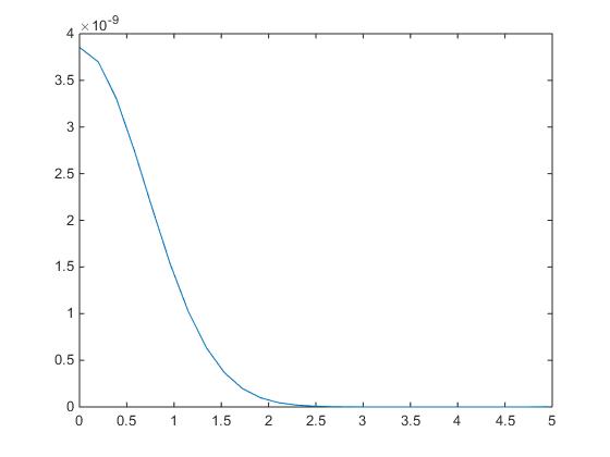
For n=10n=10, α=0.7\alpha=0.7, γ=0.5\gamma=0.5 we get next results.

xx Numerical calculation of Exact value of Absolute error
𝐈γα​e−x2\mathbf{I}^{\alpha}_{\gamma}e^{-x^{2}}, α=0.7\alpha=0.7, γ=0.5\gamma=0.5 𝐈γα​e−x2\mathbf{I}^{\alpha}_{\gamma}e^{-x^{2}}, α=0.7\alpha=0.7, γ=0.5\gamma=0.5
0,01 6,020591617 6,020591621 3,84693E-09
0,2 6,004767496 6,0047675 3,69646E-09
0,39 5,962266113 5,962266116 3,30447E-09
0,58 5,898170155 5,898170158 2,74828E-09
0,77 5,81943073 5,819430732 2,1265E-09
0,96 5,733357751 5,733357752 1,53078E-09
1,15 5,646313464 5,646313465 1,02519E-09
1,34 5,562932683 5,562932684 6,38767E-10
1,53 5,485940593 5,485940594 3,7027E-10
1,72 5,416426922 5,416426922 1,99684E-10
1,91 5,354341757 5,354341757 1,00189E-10
2,1 5,299001572 5,299001572 4,67759E-11
2,29 5,249480524 5,249480524 2,03046E-11
2,48 5,204851927 5,204851927 8,22364E-12
2,67 5,16430296 5,16430296 3,09441E-12
2,86 5,127166869 5,127166869 1,09246E-12
3,05 5,0929132 5,0929132 3,58824E-13
3,24 5,061123119 5,061123119 1,14575E-13
3,43 5,031463853 5,031463853 4,44089E-14
3,62 5,003667528 5,003667528 1,42109E-14
3,81 4,977515233 4,977515233 5,32907E-15
4 4,952825466 4,952825466 2,66454E-15
4,19 4,929445799 4,929445799 7,99361E-15
4,38 4,9072468 4,9072468 1,33227E-14
4,57 4,886117511 4,886117511 3,81917E-14
Refer to caption
Рис. 1: 𝐈γα​e−x2=Γ⁡(γ+12−α)22​α​Γ​(γ+12)​e1−x2​F1​(α,γ+12,x2)\mathbf{I}^{\alpha}_{\gamma}e^{-x^{2}}=\frac{\Gamma\left(\frac{\gamma+1}{2}-\alpha\right)}{2^{2\alpha}\Gamma\left(\frac{\gamma+1}{2}\right)}e^{-x^{2}}\,_{1}F_{1}\left(\alpha,\frac{\gamma+1}{2};x^{2}\right).
Refer to caption
Рис. 2: Absolute error of numerical calculation of 𝐈γα​e−x2\mathbf{I}^{\alpha}_{\gamma}e^{-x^{2}}.

As for numerical scheme for Bessel–Riesz fractional derivative we should notice that just as ordinary shift operators can be expanded in powers of the differentiation operator, the operators Tyxγ\,{}^{\gamma}T_{x}^{y} can be expanded in powers of the Bessel operator by the formula [16]

Tyxγ​f​(x)=∑k=0mφk​(y)​Bγk​f​(x)+Rm​(x,y),\,{}^{\gamma}T_{x}^{y}f(x)=\sum\limits_{k=0}^{m}\varphi_{k}(y)B_{\gamma}^{k}f(x)+R_{m}(x,y),

where

φk​(x)=1k!​Γ⁡(γ+12)Γ⁡(γ+12+k)​(x2)2​k,\varphi_{k}(x)=\frac{1}{k!}\frac{\Gamma\left(\frac{\gamma+1}{2}\right)}{\Gamma\left(\frac{\gamma+1}{2}+k\right)}\left(\frac{x}{2}\right)^{2k},
Rm​(x,y)=φm+1​(y)​Bγm+1​f​(ξ)|ξ=x+θ​y,−1<θ<1.R_{m}(x,y)=\varphi_{m+1}(y)B_{\gamma}^{m+1}f(\xi)|_{\xi=x+\theta y},\qquad-1<\theta<1.

We have

φ0​(x)=1,φ1​(x)=Γ⁡(γ+12)Γ⁡(γ+12+1)​(x2)2=x22​(γ+1).\varphi_{0}(x)=1,\qquad\varphi_{1}(x)=\frac{\Gamma\left(\frac{\gamma+1}{2}\right)}{\Gamma\left(\frac{\gamma+1}{2}+1\right)}\left(\frac{x}{2}\right)^{2}=\frac{x^{2}}{2(\gamma+1)}.

Then

Ttxγ​f​(x)−f⁡(x)=t22​(γ+1)​Bγ​f​(ξ)|ξ=x+θ​t\,{}^{\gamma}T_{x}^{t}f(x)-f(x)=\frac{t^{2}}{2(\gamma+1)}B_{\gamma}f(\xi)|_{\xi=x+\theta t}

and for 0<α<10<\alpha<1

(𝐁γαf)(x)=−12​(γ+1)​d1,γ​(α)∫0∞t1−2​α(Bγf(ξ)|ξ=x+θ​t)dt\left(\mathbf{B}_{\gamma}^{\alpha}f\right)(x)=-\frac{1}{2(\gamma+1)d_{1,\gamma}(\alpha)}\int\limits_{0}^{\infty}t^{1-2\alpha}(B_{\gamma}f(\xi)|_{\xi=x+\theta t})\,\>dt

converges absolutely for f∈Se​vf\in S_{ev}. Since Se​vS_{ev} is dense in LpγL_{p}^{\gamma} we can also take function f∈Lpγf\in L_{p}^{\gamma}, 1≤p<∞1\leq p<\infty.

Example 2. Let find 𝐁γα​jγ−12​(x)\mathbf{B}_{\gamma}^{\alpha}j_{\frac{\gamma-1}{2}}(x) for γ=2\gamma=2, 0<α<10<\alpha<1. Using formula (10) and the fact that j1/2​(x)=sin⁡xxj_{1/2}(x)=\frac{\sin{x}}{x} we get:

(𝐁γα​f)​(x)=1d1,2​(α)​sin⁡xx​∫0∞t−sin⁡tt2​α+2​𝑑t=\left(\mathbf{B}_{\gamma}^{\alpha}f\right)(x)=\frac{1}{d_{1,2}(\alpha)}\frac{\sin{x}}{x}\int\limits_{0}^{\infty}\frac{t-\sin{t}}{t^{2\alpha+2}}\>dt=
=Γ⁡(−1−2​α)​cos⁡(α​π)​1d1,2​(α)​sin⁡xx=π​cos⁡(α​π)Γ⁡(2​α+2)​sin⁡(2​π​α)​1d1,2​(α)​sin⁡xx,=\Gamma(-1-2\alpha)\cos(\alpha\pi)\frac{1}{d_{1,2}(\alpha)}\frac{\sin{x}}{x}=\frac{\pi\cos(\alpha\pi)}{\Gamma(2\alpha+2)\sin(2\pi\alpha)}\frac{1}{d_{1,2}(\alpha)}\frac{\sin{x}}{x},

since

d1,2​(α)=π​Γ​(32)22​α+1​Γ​(32+α)​Γ​(12+α)​1sin⁡α​πd_{1,2}(\alpha)=\frac{\pi\,\Gamma\left(3\over 2\right)}{2^{2\alpha+1}\,\Gamma\left(\frac{3}{2}+\alpha\right)\Gamma(\frac{1}{2}+\alpha)}\frac{1}{\sin{\alpha\pi}}

we get

(𝐁γα​f)​(x)=22​α​Γ​(32+α)​Γ​(12+α)Γ⁡(32)​Γ​(2​α+2)​sin⁡xx.\left(\mathbf{B}_{\gamma}^{\alpha}f\right)(x)=\frac{2^{2\alpha}\Gamma\left(\frac{3}{2}+\alpha\right)\Gamma(\frac{1}{2}+\alpha)}{\Gamma\left(3\over 2\right)\Gamma(2\alpha+2)}\frac{\sin{x}}{x}.

For n=10000n=10000, α=0.2\alpha=0.2, γ=2\gamma=2 we get next results.

xx Numerical calculation of Exact value of Absolute error
𝐁γα​j12​(x)\mathbf{B}^{\alpha}_{\gamma}j_{\frac{1}{2}}(x), α=0.2\alpha=0.2, γ=2\gamma=2 𝐁γα​j12​(x)\mathbf{B}^{\alpha}_{\gamma}j_{\frac{1}{2}}(x), α=0.2\alpha=0.2, γ=2\gamma=2
0,01 1,397316 1,41372 0,016428
0,3 1,397316 1,392633 0,016183
0,59 1,397316 1,333139 0,015491
0,88 1,397316 1,238213 0,014388
1,17 1,397316 1,112569 0,012928
1,46 1,397316 0,96238 0,011183
1,75 1,397316 0,794917 0,009237
2,04 1,397316 0,618117 0,007183
2,33 1,397316 0,440132 0,005114
2,62 1,397316 0,26886 0,003124
2,91 1,397316 0,11151 0,001296
3,2 1,397316 -0,02579 0,0003
3,49 1,397316 -0,1383 0,001607
3,78 1,397316 -0,22288 0,00259
4,07 1,397316 -0,27812 0,003232
4,36 1,397316 -0,30433 0,003536
4,65 1,397316 -0,30344 0,003526
4,94 1,397316 -0,2788 0,00324
5,23 1,397316 -0,2349 0,00273
5,52 1,397316 -0,17703 0,002057
5,81 1,397316 -0,11089 0,001289
6,1 1,397316 -0,04222 0,000491
6,39 1,397316 0,023587 0,000274
6,68 1,397316 0,081794 0,00095
6,97 1,397316 0,128612 0,001495
7,26 1,397316 0,161377 0,001875
7,55 1,397316 0,178666 0,002076
7,84 1,397316 0,180307 0,002095
8,13 1,397316 0,16731 0,001944
8,42 1,397316 0,141717 0,001647
8,71 1,397316 0,106388 0,001236
9 1,397316 0,064737 0,000752
9,29 1,397316 0,020448 0,000238
9,58 1,397316 -0,02281 0,000265
Refer to caption
Рис. 3: 𝐁γα​j12​(x)=22​α​Γ​(32+α)​Γ​(12+α)Γ⁡(32)​Γ​(2​α+2)​sin⁡xx.\mathbf{B}^{\alpha}_{\gamma}j_{\frac{1}{2}}(x)=\frac{2^{2\alpha}\Gamma\left(\frac{3}{2}+\alpha\right)\Gamma(\frac{1}{2}+\alpha)}{\Gamma\left(3\over 2\right)\Gamma(2\alpha+2)}\frac{\sin{x}}{x}..
Refer to caption
Рис. 4: Absolute error of numerical calculation of 𝐁γα​j12​(x)\mathbf{B}^{\alpha}_{\gamma}j_{\frac{1}{2}}(x).

5 Conclusion

On the Hankel transform basis using the integral transform compositional method proposed by V.V.Katrakhov and S.M. Sitnik, fractional powers of the Bessel operator are constructed. This article also discussed numerical methods for fractional powers of Bessel operator. Differential and integral operators presented in the article include one-dimensional Riesz B-potentials and Bessel–Riesz fractional derivative.

Список литературы

  • [1] Fitouhi A., Jebabli I., Shishkina E. L., Sitnik S. M. Applications of integral transforms composition method to wave-type singular differential equations and index shift transmutations, Electron. Journal Differential Equations. 2018, 130, pp. 1–27.
    https://zbmath.org/?q=an:06895433 (In English)
  • [2] Ситник С. М., Шишкина Э. Л. Метод операторов преобразования для дифференциальных уравнений с операторами Бесселя, 2019, Физматлит, Москва, 221 стр. Sitnik S. M., Shishkina E. L. Transmutation operators method for differential equations with Bessel operators, 2019, Fizmathlit, Moscow 221 p. (In Russian)
  • [3] Shishkina E. L., Sitnik S. M. Transmutations, singular and fractional differential equations with applications to mathematical physics, 2020, Elsevier, Amsterdam, 592 p. (In English)
  • [4] Shishkina E. L., Sitnik S. M. On fractional powers of Bessel operators, Journal of Inequalities and Special Functions, Special issue To honor Prof. Ivan Dimovski’s contributions, 2017, 8, 1, pp. 49–67.
    https://mathscinet.ams.org/mathscinet-getitem?mr=3636758 (In English)
  • [5] Ситник С. М., Шишкина Э. Л. О дробных степенях оператора Бесселя на полуоси, Сиб. электрон. матем. изв., 2018, 15, c. 1–10.
    Sitnik S. M., Shishkina E. L. On fractional powers of the Bessel operator on semiaxis, Siberian Electronic Mathematical Reports, 2018, 15, pp. 1–10.
    https://zbmath.org/?q=an:1390.26012
  • [6] Ляхов Л. Н. Обращение B-потенциалов Рисса, Докл. АН СССР, 1991, 321, 3, с. 466–469. Lyakhov L. N. Inversion of the B-Riesz potentials Dokl. Akad. Nauk SSSR, 1991, 321, 3, pp. 466–469.
    https://zbmath.org/?q=an:0792.31005 (In Russian)
  • [7] Ляхов Л. Н., Пространства B-потенциалов Рисса, Докл. АН СССР, 1994, 334, 3, с. 278–280. Lyakhov L. N. Spaces of Riesz B-potentials, Dokl. Akad. Nauk SSSR, 1994, 334, 3, pp. 278–280.
    https://zbmath.org/?q=an:0864.46019 (In Russian)
  • [8] Ляхов Л. Н. Описание пространства B-потенциалов Рисса Uαγ​(Lpγ)U^{\gamma}_{\alpha}(L_{p}^{\gamma}) с помощью B-производных порядка 2​[α/2]2[\alpha/2], Докл. РАН, 1995, 341, 2, с. 161–165. In Russian Lyakhov L. N. Description of the Riesz B-potential space Uαγ​(Lpγ)U^{\gamma}_{\alpha}(L_{p}^{\gamma}) using B-derivatives of order 2​[α/2]2[\alpha/2], Dokl. RAN, 1995, 341, 2, p. 161–165.
    https://zbmath.org/?q=an:0889.46033 (In Russian)
  • [9] Ляхов Л. Н., Половинкина М. В. Пространство весовых потенциалов Бесселя, Тр. МИАН, 2005, 250, c. 192–197. Lyakhov L. N., Polovinkina M. V. The Space of Weighted Bessel Potentials, Proc. Steklov Inst. Math., 2005, 250, pp. 192–197.
    https://zbmath.org/?q=an:1127.47044 (In Russian)
  • [10] Гулиев В. С. Теоремы вложения для весовых пространств Соболева B-значных функций, Докл. РАН, 1994, 338, 4, с. 440–443. Guliev V. S. Embedding theorems for weighted Sobolev spaces of B-valued functions, Dokl. Math., 1994, 338, 4, pp. 440–443.
    https://zbmath.org/?q=an:0876.46024 (In Russian)
  • [11] Riesz M. L’intégrale de Riemann-Liouville et le probleme de Cauchy, Acta Math., 1949, 81, 1–2, pp. 1–223. (In French)
  • [12] Fremberg M. E. Some Applications of the Riesz Potential to the Theory of the Electromagnetic Field and the Meson field, Proc. R. Soc. Lond., 1946, 188, pp. 18–31 (In English)
  • [13] Caffarelli L., Silvestre L. An Extension Problem Related to the Fractional Laplacian, Communications in Partial Differential Equations, 2006, 32, 8, pp. 1245–1260. (In English)
  • [14] Enciso A., Gonzalez M. del Mar, Vergara B. Fractional powers of the wave operator via Dirichlet-to-Neumann maps in anti-de Sitter spaces Journal of Functional Analysis, 2016, 273, 6, pp. 2144–2166. (In English)
  • [15] Киприянов И. А. Сингулярные эллиптические краевые задачи, 1997, Наука, Москва, 196 c. Kipriyanov I. A. Singular Elliptic Boundary Value Problems, 1997, Nauka, Moscow, 196 p. (In Russian)
  • [16] Левитан Б. М. Разложение по функциям Бесселя в ряды и интегралы Фурье, УМН, 1951, 6, 2(42), c. 102–143. In Russian Levitan B. M. Expansion in Fourier Series and Integrals with Bessel Functions, Uspekhi Mat. Nauk, 1951, 6, 2(42), pp. 102–143.
    https://zbmath.org/?q=an:0043.07002 (In Russian)
  • [17] Abramowitz M., Stegun I. A. Handbook of Mathematical Functions with Formulas, Graphs and Mathematical Tables, 1972, Dover Publ., Inc., New York, 1060 p. (In English)
  • [18] Prudnikov A. P., Brychkov Yu. A., Marichev O. I. Integrals and series. 1, Elementary Functions, 1992, Gordon & Breach Sci. Publ., New York, 640 p. (In English)
  • [19] Prudnikov A. P., Brychkov Yu. A., Marichev O. I. Integrals and Series, Vol. 2, Special Functions, 1990, Gordon & Breach Sci. Publ., New York, 753 p. (In English)
  • [20] Kratzer A., Franz W. Transzendente Funktionen, 1960, Akademische Verlagsgesellschaft, Leipzig, 375 p. (In German)
  • [21] Abramowitz M., Stegun I. A. Handbook of Mathematical Functions with Formulas, Graphs and Mathematical Tables, 1972, Dover Publ., Inc., addr New York, 1060 p. (In English)
  • [22] Самко С. Г. Килбас А. А., Маричев О. И. Интегралы и производные дробного порядка и некоторые их приложения, 1987, Наука и техника, Минск, 688 с. Samko S. G. Kilbas A. A., Marichev O. I. Integrals and derivatives of fractional order and some of their applications, 1987, Nauka i tekhnika, Minsk, 688 p.
    https://zbmath.org/?q=an:0617.26004 (In Russian)
  • [23] Davis P., Rabinowitz P. Methods of Numerical Integration, 2007, Dover Publ., Inc., New York, 612 p. (In English)
  • [24] Rabinowitz P., Weiss G. Tables of Abscissas and Weights for Numerical Evaluation of Integrals of the form ∫0∞exp⁡(−x)​xn​f​(x)​𝑑x\int\limits_{0}^{\infty}\exp(-x)x^{n}f(x)\,dx, Mathematical Tables and Other Aids to Computation, 1959, 13, p. 285–294. (In English)
  • [25] Szegő G. Orthogonal polynomials, 1975, Amer. Math. Soc. Colloq. Publ., vol. 23, Amer. Math. Soc., Providence, 432 p. (In English)