Probing Nuclear and Circumnuclear Properties of NGC 6300 using X-ray Observations2020Probing Nuclear and Circumnuclear Properties of NGC 6300 using X-ray Observations–Probing Nuclear and Circumnuclear Properties of NGC 6300 using X-ray Observations
Abstract
We present the results obtained from a detailed X-ray timing and spectral analysis of Seyfert 2 galaxy NGC 6300 by using observations with the Suzaku, Chandra and NuSTAR observatories between 2007 and 2016. We calculate variance, rms fractional variability of the source in different energy bands and find variabilities in various energy bands. Spectral properties of the source are studied by using various phenomenological and physical models. The properties of the Compton clouds, reflection, Fe K line emission and soft X-ray excess are studied in detail. Several physical parameters of the source are extracted and investigated to establish the presence/absence of any correlation between them. We also investigate the nature of the circumnuclear ‘torus’ and find that the torus is not uniform, rather clumpy. The observed changes in the line-of-sight column density can be explained in terms of transiting clouds. The iron line emitting region is found to be different in the different epoch of observations. We also observe that the torus and the nucleus independently evolve over the years.
Keywords:
galaxies: active – galaxies: Seyfert – X-rays: galaxies – X-rays: individual: NGC 63001 Introduction
Active galactic nuclei (AGNs) are the most energetic persistent objects in the universe. The AGNs are powered by the accreting supermassive black holes (SMBH) which reside at the centre of each galaxy (Rees 1984). The matter from the surrounding medium is accreted in the form of a geometrically thin, optically thick accretion disc around the blackhole (Shakura & Sunyaev 1973), also known as the standard disc. The accretion disc, in case of AGNs, predominately radiates in the UV/optical wavebands and creates the so-called ‘big-blue-bump’ in the broadband spectral energy distribution (SED). The X-rays, on the other hand, are emitted from a Compton cloud located within a few tens of Schwarzschild radii around the central engine (Haardt & Maraschi 1991; Fabian et al. 2015). The X-rays can be produced by the inverse-Compton scattering of the UV/optical photons originating from the accretion disc. The hard X-ray photons are reflected at the relatively cold matter and produce Fe fluorescent line (George & Fabian 1991; Matt et al. 1991). Thus, along with the primary X-ray continuum, a reflection hump at 15-30 keV energy range, and a Fe fluorescent line at 6.4 keV are observed in the X-ray spectrum of AGNs. An additional soft X-ray (< 2 keV) component, known as ‘soft excess’ is often observed (Halpern 1984; Arnaud et al. 1985; Singh et al. 1985) in the AGNs spectra. The ‘soft excess’ could have a completely different origin than the primary continuum, and is often associated with the host galaxy. However, more recent studies (Chevallier et al. 2006; Sobolewska & Done 2007) indicate that the ‘soft-excess’ could be generated via reflection mechanism or due to the variable nature of the hydrogen column density () along the line of sight. Inverse Comptonization by warm and optically thick region (Mehdipour et al. 2011) and relativistic blurred reflection of the hot coronal photons by the inner disc (Nardini et al. 2011) are also considered to be the origin of the soft excess . Lohfink et al. 2012 suggested that hot corona to be the origin of the soft excess. García et al. 2019 explored both the possibilities, i.e. relativistic reflection as well as Comptonization form warm corona in Mrk 509. The AGNs also produce powerful relativistic jets which are best observed in radio bands. About 15 per cent AGNs show relativistic jets, leading to a classification of radio-loud and radio-quiet AGNs (Urry & Padovani 1995). Recently, Panessa et al. 2016 reported that from the total AGN population, about per cent galaxies are the radio galaxies.
AGNs are classified as type-I or type-II based on the observation of broad line emission (originate in the broad line emitting region or BLR) or narrow line emission (originate from narrow line emitting region or NLR) in the optical wavebands (Antonucci 1993). In type-I AGN, both broad lines and narrow lines are observed, while in type-II AGN, only narrow lines are observed in the optical spectra. Observation of broad lines in the polarized light in NGC 1068 revealed that the BLR is obstructed by an absorbing dusty ‘torus’ surrounding the AGN (Antonucci & Miller 1985). This leads to the unified model for AGN, where the classification is due to the orientation effect. The unified model of AGN from the optical wavebands transforms into the X-ray wavebands as the hydrogen column density () in the line-of-sight of the absorbing material. The type-I AGNs are observed in unobstructed way with cm-2, while the type-II AGNs are observed through the obstruction where cm-2. In the case of type-II AGNs, a dusty torus around the accretion disc is considered as the major absorbing medium along the line-of-sight of the observer although the possibility of contribution from NLRs and BLRs towards total can not be ignored. The obscuring torus is characterized by its hydrogen column density (). If atoms , the torus is considered as Compton thick; otherwise, the torus is Compton thin. Generally, photons with energy keV suffers absorption and above keV, the unabsorbed spectrum is expected. The absorption of X-rays increases as the column density of absorbing material increases. In the case of torus geometry, flux suppression in the energy range below 10 keV gets flatten off in case of Compton-thick source, i.e. cm-2, as there is always reflected flux contribution from the torus irrespective of the obscuration level of the torus (Brightman & Nandra 2011).
Seyfert 2 galaxies are the radio-quiet type-II AGNs (Netzer 2013). In this case, a dusty torus surrounds the circumnuclear region. It is believed that the ‘torus’ is located far away (a few parsecs) from the nucleus. In general, the nature of the torus does not change over the years. Although, for several AGNs, it is observed that the opacity of the torus changes from Compton-thin to Compton-thick and vice-versa in a timescale ranging from months to years (Risaliti et al. 2002; Matt, Guainazzi & Maiolino 2003). This type of AGNs are known as changing-look AGN. The variation of column density is believed to be occurred due to the transition of cloud along the line-of-sight. The location of these transiting clouds commensurate with the outer region of the BLR or dusty inner torus and sometimes with the inner BLR (Markowitz et al. 2014). Hernández-García et al. 2015 showed that Compton-thin and changing-look AGNs show more variabilities than the Compton-thick AGN.
NGC 6300 is a nearby Seyfert 2 galaxy with (Meyer et al. 2004). It is located at R.A. = ; DEC = ° (Skrutskie et al. 2006). It is a ring, barred spiral galaxy and classified as SBb-type galaxy from its morphology. NGC 6300 was observed a few times in X-ray bands with the RXTE (Leighly et al. 1999), BeppoSAX (Matsumoto et al. 2004) and XMM-Newton (Guainazzi 2002), in February 1997, August 1999 and March 2001, respectively. From the variability studies with the XMM-Newton, the mass of NGC 6300 was estimated to be . The relation yields the mass of NGC 6300 to be . However, with various uncertainties, the mass is estimated to be (Awaki et al. 2005). Khorunzhev et al. 2012 estimated the mass of the BH to be from mass-bulge luminosity correlation. The NIR study of the molecular radial velocity yields the mass of the BH as (Gaspar, et al. 2019).
In this article, we study the Seyfert 2 galaxy NGC 6300 by using observations between 2007 & 2016 at five epochs (2007, 2009, 2013, January 2016 & August 2016) with the Suzaku, Chandra, and NuSTAR observatories. We investigate the characteristics of the nucleus as well as the nature of the circumnuclear torus. In §2, we briefly discuss the observations and data reduction processes. In §3, we present timing and spectral analysis methods and the corresponding results. In §4, we discuss our findings. Finally, we draw our conclusions in §5.
2 Observation and Data Reduction
| ID | Date | Obs. ID | Instrument | Exposures |
|---|---|---|---|---|
| (yyyy-mm-dd) | (ks) | |||
| S1 | 2007-10-17 | 702049010 | Suzaku | 82.5 |
| C1 | 2009-06-03 | 10289 | Chandra/ACIS | 10.2 |
| C2 | 2009-06-07 | 10290 | Chandra/ACIS | 9.8 |
| C3 | 2009-06-09 | 10291 | Chandra/ACIS | 10.2 |
| C4 | 2009-06-10 | 10292 | Chandra/ACIS | 10.2 |
| C5 | 2009-06-14 | 10293 | Chandra/ACIS | 10.2 |
| N1 | 2013-02-25 | 60061277002 | NuSTAR | 17.7 |
| N2 | 2016-01-24 | 60261001002 | NuSTAR | 20.4 |
| N3 | 2016-08-24 | 60261001004 | NuSTAR | 23.5 |
We searched and acquired the publicly available archival data of NGC 6300 from Suzaku, Chandra and Nustar observatories by using HEASARC11 1 http://heasarc.gsfc.nasa.gov/.
2.1 Suzaku
NGC 6300 was observed with Suzaku on 2007 October 17 (Obs ID: 702049010). The Suzaku observatory consisted of two sets of instruments: the X-ray Imaging Spectrometer (XIS) (Koyama et al. 2007) and the Hard X-ray Detector (HXD) (Takahashi et al. 2007). There are four units of XIS among which XIS-0, XIS-2, and XIS-3 were front-side-illuminated CCDs (FI-XISs), while XIS-1 was back-side-illuminated one (BI-XIS). The HXD was a non-imaging Instrument consisting of Si PIN photo-diodes and GSO scintillation counters. We followed22 2 http://heasarc.gsfc.nasa.gov/docs/suzaku/analysis/abc/ standard procedures and recommended screening criteria while extracting Suzaku/XIS spectra and light-curves. We reprocessed the event files by using the latest calibration data files 33 3 http://www.astro.isas.jaxa.jp/suzaku/caldb/, released on 2014-02-03, through the software package FTOOLS 6.25. We chose a circular region with a radius of 210 arcsecs and source coordinates as the centre, for source extraction. The background spectra were extracted from source-free regions by selecting a circular region of 210 arcsecs radius. With the xisrmfgen and xisarfgen task, we generated Response matrices and ancillary response files, respectively. As XIS-2 was not operational, the data from the other three XISs are used in the present analysis. The keV front-illuminated XIS-0 and XIS-3 spectra are co-added using the addascaspec task, whereas the keV back-illuminated XIS-1 spectrum was treated separately. The XIS spectra in keV range was ignored due to the presence of known Si edge. All the spectra are re-binned to achieve 20 counts per channel bins by using the grppha task. For Suzaku HXD/PIN spectra, cleaned event files were generated using the aepipeline task. With the hxdpinxbpi task, the deadtime corrected source and background spectra were generated. The background spectra included non-X-ray background (nxb; Fukazawa et al. 2009) and the simulated cosmic X-ray background (cxb; Gruber et al. 1999). We used HXD/PIN spectrum in keV energy range in our analysis.
2.2 Chandra
The Chandra/ACIS observed NGC 6300 five times between 2009 June 03 and 2009 June 14. We summarized these observations in Table 1. All the observations were carried out in Faint data mode. The data were processed with the Chandra Interactive Analysis of Observations tools (CIAO v.4.1144 4 https://cxc.harvard.edu/ciao/download/;(Fruscione et al. 2006; Huenemoerder et al. 2011)) by using corresponding Calibration Database (CALDB v.4.8.5)55 5 https://cxc.harvard.edu/ciao/download/caldb.html. We first reprocessed the level-2 event files by applying the updated calibration data using CIAO script chandra_repro 66 6 https://cxc.cfa.harvard.edu/ciao/ahelp/chandra_repro.html. After that, we used the CIAO tool axbary to apply the barycentre correction on the reprocessed level-2 event files. We considered a circular region of 2.46 arcsec radius, centred at the source coordinates, to extract the source light curves and spectra. The background light curves and spectra were extracted by selecting a circular region of 10 arcsec radius and away from the source. Finally, we used specextract and dmextract to extract the spectra and light curves of the source and background, respectively. To check the amount of pile-up in each observation, we used the CIAO tool PILEUP_MAP. Although it is less than 10 per cent, we account this effect in spectral fitting by using the convolution model pileup (Davis 2001) 77 7 https://heasarc.gsfc.nasa.gov/xanadu/xspec/manual/node304.html with all spectral model, with frame time set to 0.5s. We did not see any changes with or without pileup model.
2.3 NuSTAR
NGC 6300 was observed with NuSTAR (Harrison et al. 2013) three times; once in 2013, and twice in 2016 (see Table 1 for details). The NuSTAR consists of two identical modules: FPMA and FPMB. Reduction of the raw data was performed with the NuSTAR Data Analysis Software (NuSTARDAS, version 1.4.1). Cleaned event files were generated and calibrated by using the standard filtering criteria with the nupipeline task and the latest calibration data files available in the NuSTAR calibration database (CALDB)88 8 http://heasarc.gsfc.nasa.gov/FTP/caldb/data/nustar/fpm/. Both the extraction radii for the source and the background products were set to be 80 arcsec. With the nuproduct task, the spectra and light-curves were extracted. The light curves were binned over 100s. Considering the background counts, we limited our spectral analysis within keV range. We re-binned the spectra to achieve 20 counts per bin by using the grppha task.
3 Results
We used Suzaku, Chandra, and NuSTAR data between 2007 and 2016 for our analysis. All the instruments have different effective area, thus, one needs to take care of this. To address this issue, we used ‘ancillary response file (arf)’ in the spectra. For the lightcurves, we used a cross-normalization factor to normalize the count rate using crab light curve. We used cross-normalization factor, , , (Madsen et al. 2015; Madsen et al. 2017).
We used the following cosmological parameters in this work: = 70 km s-1 Mpc -1, = 0.73, and = 0.27 (Bennett et al. 2003).
3.1 Timing Analysis
We considered all the X-ray light curves obtained from the Suzaku, Chandra and NuSTAR observations of NGC 6300 with 100 s bin for timing analysis. We segregated the total energy bins into various segments for variability analysis. We divided the low energy data ( keV) into two energy bands, namely keV and keV for variability analysis for Suzaku/XIS and Chandra observations. The NuSTAR data ( keV range) were divided into two chunks: keV and keV ranges for variability analysis. To examine the time delay between the Fe Kα line and continuum, we considered the light curve of keV with the Fe line counts (in keV energy band) for NuSTAR observations. The keV light curves were taken into account to analyze the variability in the high energy part.
| ID | ||||||
|---|---|---|---|---|---|---|
| () | ||||||
| S1(0.5-3) | 198 | 0.196 | 0.021 | 9.40 | - | |
| C1(0.5-3) | 18 | 0.020 | 0.002 | 9.11 | ||
| C2(0.5-3) | 20 | 0.027 | 0.005 | 6.00 | ||
| C3(0.5-3) | 19 | 0.022 | 0.002 | 9.88 | ||
| C4(0.5-3) | 21 | 0.028 | 0.002 | 12.1 | ||
| C5(0.5-3) | 20 | 0.020 | 0.002 | 9.11 | - | |
| S1(3-10) | 203 | 0.49 | 0.11 | 4.31 | ||
| C1(3-10) | 21 | 0.09 | 0.02 | 4.55 | ||
| C2(3-10) | 20 | 0.30 | 0.15 | 2.08 | ||
| C3(3-10) | 22 | 0.21 | 0.01 | 2.32 | ||
| C4(3-10) | 21 | 0.30 | 0.12 | 2.56 | ||
| C5(3-10) | 21 | 0.25 | 0.07 | 3.65 | ||
| N1(3-10) | 44 | 1.01 | 0.32 | 3.17 | ||
| N2(3-10) | 49 | 0.74 | 0.20 | 3.75 | ||
| N3(3-10) | 62 | 0.84 | 0.31 | 2.68 | ||
| N1(10-40) | 44 | 0.63 | 0.27 | 2.33 | ||
| N2(10-40) | 49 | 0.52 | 0.19 | 2.61 | ||
| N3(10-40) | 62 | 0.93 | 0.26 | 3.60 | - |
3.1.1 Variablility
To examine the temporal variability in X-ray emission from NGC 6300, in the different energy bands during the period of 17th October 2007 to 24th August 2016, we estimated numerous parameters. The fractional variability (Edelson et al. 1996; Nandra et al. 1997; Edelson et al. 2001; Edelson et al. 2012; Vaughan et al. 2003; Rodríguez-Pascual et al. 1997) for a light curve of count/s with finite measurement error of length with a mean and standard deviation is given by:
| (1) |
where is excess variance (Nandra et al. 1997; Edelson et al. 2002), an estimator of the intrinsic source variance and is given by:
| (2) |
The normalized excess variance is given by . The uncertainties in and are taken from Vaughan et al. 2003 and Edelson et al. 2012. The peak to peak amplitude is defined as (where and are the maximum and minimum flux, respectively) to investigate the variability in the X-ray light curves.
The X-ray photons from NGC 6300 in different energy bands (0.5–3 keV, 3–10 keV, 10–40 keV ranges) showed different magnitude of variabilities. The results are shown in Table 2. From the low energy part ( keV range), we obtained an average value of which has a range from to . However, for higher energy part (3–10 keV range), we observed , ranging from to . Thus, the high energy part showed fewer variabilities in terms of the average values and range of . Although, exhibited opposite nature. A trend of increasing normalized excess variance can be seen from Table 2. It should also be noted that the errors of (calculated considering variance ) are larger than the values for 0.5–3 keV energy band. Thus, the conclusions solely based on would be erroneous.
We calculated the fractional variability () in terms of normalized excess variance () to investigate the variabilities in different wavebands. These quantities describe the variability strength present in AGN light curves. Though and represent similar information, the latter was used as is independent of the signal-to-noise ratio of the light curve. From Table 2, we can infer that NGC 6300 had a constant decrease of variability strength with increasing energy (; ; ) over the entire period of time.
3.1.2 Correlation
In order to investigate the physical connection between the Fe line and the X-ray continuum, we computed the Pearson correlation coefficient () and Spearman’s rank correlation coefficient () using the NuSTAR observation. Quantitive analysis of the correlation based on the Pearson coefficient provided a degree of linear correlation between the Fe-line emission and the X-ray continuum. We correlated keV light curves (for X-ray continuum) with the Fe line light curves. The Fe line light curves are computed in the energy range of keV. The positive and negative values of the Pearson coefficient for all three observations indicated a very weak linear correlation between the Fe-flux and the X-ray continuum. This implies a plausible disjoint mechanism involved in the emission of the Fe line and the X-ray continuum. We estimated the Spearman’s rank correlation to further quantify the degree of correlation between the Fe flux and X-ray continuum. It reflects a similar result for the first two observations. The result of this correction study is quoted in Table 3.
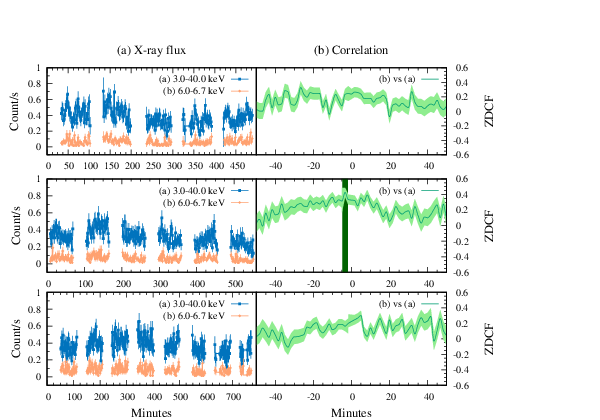
We also investigate the time-delay between the Fe-line flux and the X-ray continuum by using the -transformed discrete correlation function (ZDCF) method fully described by Alexander 1997 99 9 http://www.weizmann.ac.il/particle/tal/research-activities/software. The ZDCF-code is publicly available for estimating the cross-correlation function of unevenly sampled light curves. We considered the X-ray light curves in keV range with the Fe-line flux for three NuSTAR observations to estimate the ZDCF coefficient. We calculated ZDCF for two different cases: omit zero lag points and include zero lag points, and in both cases, we got a similar result. The values of ZDCF coefficient with time delay is presented in Table 3. Also, the variation of coefficient with time delay is shown in Figure 1. Although there is no prominent peak in the correlation function, we found a moderate peak at the time delay of minutes for the first observation with ZDCF coefficient value of and peak at minutes for second observation with ZDCF coefficient value of . In the case of third observation, we did not notice any peak in the correlation function.
| ID | |||||
|---|---|---|---|---|---|
| (min) | |||||
| N1 | 0.2385 | 0.1835 | .0115 | ||
| N2 | 0.3490 | 0.3494 | < .001 | ||
| N3 | -0.2700 | 0.3676 | < .001 |
3.2 Spectral Analysis
Spectral analysis of data obtained from the Suzaku, Chandra and NuSTAR observations of NGC 6300 was carried out by using the software package XSPEC v12.10 (Arnaud 1996). For spectral fitting, we explored several phenomenological and physical models in order to understand the core region of NGC 6300. We used powerlaw, compTT (Titarchuk 1994), pexrav (Magdziarz & Zdziarski 1995), and MYTORUS (Murphy & Yaqoob 2009) models to approximate the primary continuum and reflection components. While fitting the data with the first three continuum models separately, a Gaussian component is considered for the iron fluorescent emission line. The soft X-ray excess observed in the spectra of many AGNs, is usually modelled with the combination of powerlaw and APEC model. The normalization parameter was tied with the primary component in order to get an idea of scattering fraction ; modelled with ‘constant’ in XSPEC. The soft excess component in XSPEC reads as: constant*(powerlaw + apec). Along with these components, we used two absorption components, namely TBabs and zTBabs (Wilms et al. 2000). TBabs was used for Galactic absorption and hydrogen column density () was fixed at (HI4PI Collaboration, et al. 2016). We calculated error for each spectral parameters with 90 per cent confidence level (1.6 ). The errors are calculated using ‘error’ command in XSPEC.
3.2.1 Power law
We started the spectral analysis with the simple powerlaw model. Our baseline model in XSPEC reads as:
TBabs1*(zTBabs2*(zpowerlaw + zGaussian) + soft excess).
We started our analysis using data from the Suzaku observation in 2007. The keV spectrum was fitted with the above spectral model. The parameters obtained from the fitting are , , an Fe line at keV with equivalent width (EW) of 114 eV and the reduced chi-square () = 1.03 (for 2549 dof). Next, we analyzed the data from the 2009 epoch when NGC 6300 was observed five times within 11 days with the Chandra observatory. We did not detect Fe K line in all five spectra. We verified this by using the ftest task in XSPEC. We fitted all the Chandra spectra by removing the Gaussian component from the baseline model. The hydrogen column density () along the line of sight varied between and . The power-law photon indices were similar during the 2009 epoch of observations. NGC 6300 was observed with the NuSTAR observatory in February 2013. The data obtained from the NuSTAR observation were fitted with the model yielding parameters such as , , an Fe line at keV with an equivalent width of 258 eV and the = 758/702. The iron line was found to be broader than the previous observations. The spectra became harder with photon indices of and during the observations in Jan 2016 and Aug 2016, respectively. The iron line width was increased to and eV during these two observations. However, the hydrogen column density was decreased in the 2016 epochs to which is almost per cent of the value of the column density during 2007 epoch of observation. In Figure 2, the powerlaw model fitted spectra are shown. In Figure 4, the contour plots for vs are shown for S1, C2, & N2. The powerlaw model fitted spectral analysis result is shown in Table 4.

3.2.2 CompTT model
The powerlaw model provided valuable information on the variations of spectral hardness and hydrogen column density over the observation duration of years. However, the fundamental properties such as electron temperature (), optical depth of the medium (), and approximate shape of accretion geometry (slab or spherical) are necessary to gain a deeper understanding of the system. To estimate these quantities, we replaced the powerlaw model with a more physical compTT model (Titarchuk 1994) in our spectral fitting. The X-ray emitting Compton cloud is characterized by the hot electron temperature () and optical depth (). The model considered here can be expressed as:
TBabs1*(zTBabs2 * (compTT + zGaussian) + soft excess).
While fitting with the compTT model, the values obtained were acceptable for all observations. We found that the electron temperature varied over the years, indicating a change in the spectral state. In fact, increased over the period of years from keV to keV. The value of the optical depth varied dramatically over the entire span of the observation duration. The optical depth remained mostly constant during the 2009 epoch except for the Chandra observation on 3 June 2009 (‘C1’). Particularly on that date, we found significantly high electron temperature (much higher than the Suzaku observation - S1) along with the higher value of the optical depth, suggesting a denser and hotter Compton cloud around the black hole.
Results presented here were obtained by considering a spherical cloud with seed photon temperature fixed at eV, which is likely to be the inner disc temperature for a BH with a mass of . We also considered the slab geometry for which the parameter variations remained reasonably consistent as obtained with the spherical geometry. Thus, the geometry of the Compton cloud remained unclear with the compTT model.
3.2.3 Pexrav
The reported inclination for of NGC 6300 is around (Leighly et al. 1999). As a high inclination source, the X-ray spectrum from the inner region is more prone to suffer reflection from the disc. To estimate the reflection coefficient over the entire period of our observation, we applied reflection model pexrav (Magdziarz & Zdziarski 1995). The pexrav model contains a powerlaw continuum and a reflected component from an infinite neutral slab. We estimated relative reflection () of the source. We fixed the photon index () with the value of obtained from the powerlaw model. We fixed abundances for heavy elements and iron at Solar value (i.e. 1). In the beginning, we froze at 0.22 (°). Later, we re-analyzed the data by fixing at 0.15 (°; obtained from MYTROUS model fit, see 3). As we could not constrain the cut-off energy of the Compton cloud, we froze it at keV. We found that during the 2007 Suzaku observation, the reflection was moderate (). However, in 2009 epoch, increased and dominated during the three observations (). During the other two observations in 2009 epoch, is estimated to be in the range of 0.8 and 1, indicating a strong reflection. The reflection hump was seen in keV energy range; thus, the value of obtained is in the range of 0.5 to 8.0 from the Chandra data and are not well constrained. The keV spectra from the NuSTARobservations in 2013 & 2016 epochs gave us a good estimation of . During all three NuSTAR observations, we found that the reflection was strong with . The model fitted results are given in Table 4.

3.2.4 MYTORUS
The AGNs are surrounded by circumnuclear absorbing clouds popularly referred to as ‘torus’. The phenomenological models do not consider the complex structure of the ‘torus’. Several physical models have been developed which account for the ‘toroidal geometry’ and calculate reflection and line spectra self-consistently (Ikeda et al. 2009; Murphy & Yaqoob 2009; Brightman & Nandra 2011; Baloković et al. 2018). We studied NGC 6300 with a physical model, namely the MYTORUS1010 10 https://www.mytorus.com/ model (Murphy & Yaqoob 2009; Yaqoob 2012) which describes an absorbing torus surrounding the nuclear region with half opening angle fixed at 60°. This model consists of three components: absorbed primary continuum or zeroth-ordered component (MYTZ), a scattered/reflected component (MYTS) and an iron fluorescent line component (MYTL; Fe K and Fe K line). The MYTORUS model can be used in two configurations: coupled and decoupled (Yaqoob 2012). The coupled configuration describes a uniform circumnuclear torus while the decoupled configuration attributes the nonuniformity in the torus shape and density profiles.
In the beginning, we tested the default or coupled configuration of the MYTORUS model. The model reads as,
TBabs(powerlaw*MYTZ + MYTS + MYTL + soft excess).
In this configuration, the equatorial hydrogen column density (), photon index of the incident primary continuum (), inclination angle (), and model normalization are tied together. As recommended, the relative normalizations of the scattered and line components are tied together, i.e. . We allowed the inclination angle () to vary freely. We found that the inclination angle varied between 76°and 82°. With this model, we achieved a good fit for all observations. The photon indices and equatorial column density obtained using this model followed a similar trend as obtained from the powerlaw model. In the MYTROUS model, the equivalent width is not a free parameter; instead, it is computed self-consistently. The full width half maxima (FWHM) and flux () of iron K line are obtained from a Gaussian convolution model gsmooth which can be used with MYTL component (for details, see Yaqoob 2012). The results obtained using this model are presented in Table 5.
Later, we tested the decoupled configuration of the MYTORUS model. This can be achieved by decoupling the column density of different components. Initially, we fixed of MYTZ component to 90°. This component describes the absorbed transmitted component. The hydrogen column density of MYTZ will provide us with a column density () along the line-of-sight. Next, we fixed inclination angle of MYTS and MYTL at 0°. The column density is decoupled from the MYTZ component. The column density of scattered component describes averaged global column density (). This component describes a component which is scattered from the backside and coming to us through the hole of a patchy torus (see Figure 2 of Yaqoob 2012). The model can be read as:
TBabs(powerlaw * MYTZ + MYTS + MYTL+ soft excess).
The Decoupled configuration did not give us a significantly deviated fit from the Coupled model. was found to follow the same trend as the Coupled model. The line-of-sight column density () was observed to follow the same pattern as . However, the averaged-global column density () was roughly constant for all nine observations. The scattering fraction () was 1.06 in 2007, which indicates that the reflection was dominating and delayed. In 2009 epoch, , which infers a weaker reflection compared to the primary emission. In 2013, & 2016 epochs, we observed from this model. This indicates that the spectra were dominated by the reflection. We calculated FWHM and line flux for Fe K line emission from the Gaussian convolution model gsmooth. We also calculated intrinsic luminosity () of the source using ‘clum’ command in XSPEC in the energy band of keV. We computed the intrinsic luminosity for MYTZ component (Yaqoob 2012). The results of this model are tabulated in Table 6. The MYTORUS model fitted (decoupled configuration) spectra are shown in Figure 3. In Figure 4, we show the contour plot for vs .
| ID | PL. norm | Line E | EW | /dof | |||||||||
|---|---|---|---|---|---|---|---|---|---|---|---|---|---|
| ( cm-2) | ( ph cm-2 s-1) | (keV) | ( ph cm2 s-1) | (eV) | () | (keV) | (keV) | ( ergs cm-2 s-1) | |||||
| S1 | 114 | 2614/2549 | |||||||||||
| C1 | 283/ 293 | ||||||||||||
| C2 | 305/ 321 | ||||||||||||
| C3 | 289/ 293 | ||||||||||||
| C4 | 295/ 315 | ||||||||||||
| C5 | 306/ 299 | ||||||||||||
| N1 | 258 | 758/ 702 | |||||||||||
| N2 | 280 | 802/ 715 | |||||||||||
| N3 | 299 | 781/ 821 |
| ID | PL. norm | EW | FWHM | /dof | |||||||
|---|---|---|---|---|---|---|---|---|---|---|---|
| ( ph cm-2 s-1) | ( cm-2) | (degree) | (eV) | ( ergs cm-2 s-1) | (km s-1) | () | (keV) | ||||
| S1 | 2476/2380 | ||||||||||
| C1 | 278/292 | ||||||||||
| C2 | 311/314 | ||||||||||
| C3 | 295/294 | ||||||||||
| C4 | 285/313 | ||||||||||
| C5 | 305/296 | ||||||||||
| N1 | 763/719 | ||||||||||
| N2 | 798/711 | ||||||||||
| N3 | 812/819 |


4 Discussion
We studied NGC 6300 between 2007 and 2016 by using the data from the Suzaku, Chandra, and NuSTAR observations. We mainly concentrate our study on the nuclear core and circumnuclear torus region. However, there is a possibility that the extra-nuclear X-ray sources could contribute to the X-ray emission and affect our analysis. The X-ray luminosity of NGC 6300 is ergs s-1. Although, the time-averaged luminosity of X-ray binaries can reach reach up to ergs s-1 (Remillard & McClintock 2006; Tetarenko et al. 2016). The maximum luminosity of an accretion powered X-ray Pulsar can reach up to ergs s-1 depending on a range of magnetic field between G (Mushtukov et al. 2015). The ultra-luminous X-ray (ULX) sources show luminosity about ergs s-1. The X-ray luminosity of supernovae can reach as high as ergs in the initial days. Thus, the luminosity of supernovae is per cent of our source of interest in this work. Even then, within the period of observations used in present work, no such events were recorded from the optical observations around the field of view of NGC 6300. Thus, contamination from these sources can be neglected for variability studies.
The positional accuracy of the Suzaku/XIS is around at 90 per cent confidence level (Uchiyama et al. 2008). At a similar confidence level, Chandra has positional accuracy depending on the brightness of the source (Beckerman et al. 2004; Broos et al. 2010). In case of NuSTAR, the positional accuracy varies between (Lansbury et al. 2017). For Suzaku and NuSTAR, there can be thousands of transient sources within the source region. The number reduces to hundreds for Chandra. Nevertheless, none of them can be as bright as the AGN core itself. Thus, the X-ray emission must originate from the nucleus (Gierliński et al. 2008).
4.1 Properties of torus
We refer the circumnuclear absorbing material as ‘torus’. It does not have to be a uniform torus; it could be a clumpy or patchy torus. We obtained the line-of-sight column density () and equatorial column density () from the powerlaw and MYTORUS-coupled model fitting, respectively. We observed that is slightly higher than . This is expected as matter density is expected to be high in the equatorial region. Nonetheless, they both show a similar trend over the years.
During the 2007 epoch, the column density was high with cm-2. It decreased over the years and after 9 years, it became almost half with cm-2. The overall column density of the absorber is found to be varying over nine years. Chandra observed the source five times within 11 days in 2009. During that epoch, the varied between cm-2 and cm-2. Considering a uniform torus around the AGN, the variation of column density within a few days remains a puzzle. However, in an alternative scenario, Risaliti et al. 2002 showed that the column density could be changed in timescale as short as a day if the torus is clumpy. To further investigate the nature of the torus, we used the decoupled configuration of the MYTORUS model. We find (see Table 6) that the line-of-sight column density () changed over the years while the global-averaged column density () remained almost same.
The variation of can be explained by the migrating clouds in the line of sight. During the Chandra observations in 2009, minimum change in the line of sight column density was cm-2 (between C1 & C2). If we assume that the column density of each cloud is cm-2, then the number of clouds in the line of sight in 2009 would be . Similarly, Guainazzi et al. 2016 reported that the number of clouds in the line of sight for Mkn 3 was in 2014. NGC 6300 is known as ‘changing look’ AGN (Matt, Guainazzi & Maiolino 2003; Guainazzi 2002). Guainazzi 2002 argued that the temporary ‘shut-off’ of the nucleus could be the reason for the ‘changing-look’. However, the transiting clouds in the line of sight would naturally explain the variation of observed flux and the line of sight column density (Yaqoob et al. 2015). The observed flux depends on both lines of sight column density and nuclear activity. Thus, the observed flux can be changed due to the transiting clouds in the line-of-sight even if the nucleus remains unchanged. Therefore, the ‘changing look’ AGN can be explained naturally by the transition of clouds in the line of sight.
Another possible explanation for variation could be the ionization of the ‘torus’. The outer surface of the torus can be ionized by the radiation from the AGN that has leaked through the clumpy torus (Guainazzi et al. 2016). LaMassa et al. 2015 showed that the transition of changing look quasar SDSS J015957.64+003310.5 could be explained by the ionization, but not with the transiting clouds. Nevertheless, in the case of NGC 6300, no ionized line was observed. Thus, it is improbable that the variable column density is due to ionization.
4.2 Nuclear Emission
We find the variability above 3 keV for NGC 6300 in all nine observations. The calculated rms fractional variability amplitude in keV or higher ( keV) energy bands for all the observations are presented in Table 2. The observed variability of the primary emission (>3 keV) is consistent with the other Seyfert 2 galaxies (Hernández-García et al. 2015).
In the case of supermassive black holes, the X-ray emission is mostly originated from the Compton cloud. The properties of the X-ray spectra (popularly charactarized with the photon index ) depend on the properties of the Compton cloud which is charactarized by hot electron temperature (), optical depth () and cut-off energy (). We obtained from the powerlaw model, and from the compTT model (see Table 4). We tried to estimate using the cutoffpl model, but were unable to constrain it. All observations indicated keV which is the upper limit of the cutoffpl model. The highecut model also failed to constrain of the source. Nevertheless, considering an isotropic electron cloud with seed photon source placed at the centre, as sugested by Petrucci et al. 2001, one can get an estimate of cutoff energy using for , and for . Using the relation and the parameters obtained from the compTT model, it can be implied that the cut-off energy might be keV and rise up neatly within this period of time. We also noticed the increase in with the time considering the simple theoretical approach. However, it would be naive to draw any conclusion based on the cut-off energy variation. The cut-off energy () could not be constrained (Leighly et al. 1999; Guainazzi 2002) by earlier observations too.
In our observation, we found during the 2007 & 2009 epochs. During these epochs, the Compton cloud temperature was keV. Later, in 2013 epoch, was found to increase, whereas the value of decreased. This is expected since the hotter Compton cloud emits harder and flatter spectrum. We found an anti-correlation between and with Pearson correlation index of -0.9187. This strong anti-correlation indicates that the hot electron cloud is the primary source for the harder spectra. The correlation is presented in Figure 5.
We calculated source intrinsic luminosity () in keV energy range and found to be varied over the years. was ergs s-1 in 2007. After that, it decreased in later epochs. varied between ergs s-1 and ergs s-1 in 2009, 2013 & 2016 epochs. The variation of accretion rate could be responsible for the variation of . To get an estimate of the accretion rate, we calculated the bolometric luminosity with bolometric correction dex (Brightman et al. 2017). We estimated the Eddington luminosity of the source as ergs s-1 assuming the mass of the BH as . The bolometric luminosity depends on the mass accretion rate as, , where is the energy conversion efficiency. The Eddington luminosity is . Thus, the mass accretion rate () in terms of Eddington mass accretion rate () is, . The Eddington ratio () is defined as . Since is the energy conversion efficiency, and . Therfore, . The observed or the Eddington ratio is consistent with other Seyfert 2 galaxies (Wu & Liu 2004; Sikora et al. 2007).
We found that the intrinsic luminosity () is strongly correlated with the Eddington ratio () with the Pearson correlation index as 0.9967. We also found a strong correlation between and with Pearson correction index of 0.7472. The correlation of and is studied by many authors (Lu & Yu 1999; Shemmer et al. 2006; Shemmer et al. 2008; Risaliti et al. 2009) and a positive correlation is found for NGC 6300 as well. We also found a correlation between and with Pearson correlation index as 0.7604. This positive correlation of and is observed in high redshift objects (Dai et al. 2004; Saez et al. 2008), but not in the local universe (Brightman & Nandra 2011).
Above three correlations (, , ) can be explained in a single framework of variable accretion rate. If the mass accretion rate increases, the radiated energy will increase, thus, the intrinsic luminosity. Hence, , or . Again, if the luminosity increases, it will cool down the Compton cloud more efficiently implying a steeper photon index, i.e. . These relations are well known for Galactic black holes (Remillard & McClintock 2006).
4.3 Reflection & Line Emission
Hard X-ray emission from the Compton cloud is reflected from a cold neutral medium surrounding the AGN (George & Fabian 1991; Matt et al. 1991). Within our spectral domain, the reflection component consists of a reflection hump and an iron fluorescent emission line. Due to higher inclination, the Seyfert 2 galaxies usually show stronger reflection than the Seyfert 1 galaxies (Ricci et al. 2011). The strength of the reflection component can be obtained from the pexrav (, relative reflection) or MYTORUS (; relative normalization of scattering) model. As the reflection hump is observed in keV, may not be constrained with the Chandra data. In this case, the MYTORUS model can constrain as both the reflected and the line emission are computed self-consistently.
Along with the reflection hump, the iron line emission is a good indicator of reflection. NGC 6300 is known to emit strong reflection component with unusually high (> 4) (Leighly et al. 1999). The reflection dominated RXTE spectrum was expected to show EW keV although the observed EW was about eV. Leighly et al. 1999 argued that the sub-solar abundances were the reason behind the observation of narrow line-width than expected. The EW of Fe fluorescent line was decreased in 1999 and 2001 observations with 140 eV and 69 eV, respectively (Guainazzi 2002; Matsumoto et al. 2004) although the relative reflection was still high.

In our analysis, the Fe K line was observed in the spectra of NGC 6300 during 2007, 2013 & 2016 epochs from the powerlaw model fitting. However, we did not detect the Fe K line in the spectra from the 2009 epochs while fitting the data with the powerlaw model. On the other hand, the MYTORUS model fitting result showed the presence of Fe line in all observations. This discrepancy arose as the MYTORUS model compute Fe line self-consistently, while an ad-hoc Gaussian component was added as Fe line in the powerlaw model. Thus, we made our discussion on the reflection and Fe K line based on the results obtained from the spectral analysis with MYTORUS model. During 2007, the iron K line was observed with an equivalent width of eV (see Table 6). In 2009 epoch, a marginally narrower line (95-114 eV) was observed from the Chandra observations. Though similar EW was observed in 2007 & 2009 epochs, a different relative scattering normalization was found. In 2007, indicates that the reflection dominates over the primary continuum. In 2009, the reflection was weaker compared to 2007 (). However, in 2013 & 2016 epochs, the reflection became stronger ( with broad EW (>300 eV). The observed EW is consistent for the reflection from a Compton thin reprocessor (Matt, Guainazzi & Maiolino 2003) for all the observations.
We found that the EW and are strongly correlated with Pearson correlation index of 0.9893. This indicates that the EW strongly depends on the strength of the reflection. The Fe K line flux is found to be strongly correlated with the EW and with Pearson correlation indices of 0.9347 and 0.9275, respectively. This suggests that the Fe-line flux strongly depends on the strength of the reflection. The EW also correlates with the Compton cloud temperature () and has a correlation value of 0.9146. From this, one can implicate that the hotter Compton cloud causes more reflection from various regions which broadens the line-width. However, the Pearson correlation index between Fe K line flux and is estimated to be -0.5187, which suggests a moderate anti-correlation. This X-ray Baldwin effect was observed in several other sources (Iwasawa & Taniguchi 1993; Ricci et al. 2013a; Boorman et al. 2018). Nonetheless, the 2009 epoch seems to exhibit outliers of the Baldwin effect for NGC 6300. The reason behind this could be a separate origin of the iron line than the other epochs.
Later, we focus on the Fe K line emitting region. We calculated the Fe K line emitting region from observed FWHM. In 2007, the FWHM of the Fe K-line was derived to be 5550 km s-1 which indicates that the line emitting region would be away from the central source, i.e. the broad-line region (BLR). In 2009, we observed a narrow FWHM (< 100 km s-1), which means the line emitting region is at , i.e. pc located near the ‘torus’ region. In 2013, the NuSTAR observations revealed a broad FWHM with 30000 km s-1. It implies that the line emitting region is away. In Jan 2016 & Aug 2016 observations, the values of FWHM were km s-1 and km s-1, respectively. In these two epochs also, the line emitting region would be and away, respectively. It is believed that the narrow Fe line is ubiquitous and can be emitted from the ‘torus’, the BLR or the accretion disc (Nandra 2006). From our analysis of NGC 6300, we found that the Fe fluorescent line was emitted from separate regions during various epochs. Guainazzi 2002 estimated the Fe K line emitting region for NGC 6300 to be in 2001, i.e. torus. During 2007, we find that the Fe-line was emitted from the BLR region. In 2009 epoch, we observed that the line emitting region as the ‘torus’. But, during 2013 and 2016 epochs, the iron line was emitted from the accretion disc. It is also possible that the narrow Fe K line was emitted from the ‘torus’ in 2013 and 2016 epochs, but, could not be detected due to the presence of broader Fe K line emission from the accretion disc.
Considering the time-delay patterns between Fe-line and continuum during 2013 and 2016 epochs (see Figure 1), one can get a rough estimate of the size of the Compton cloud. Since the delay between these two is minimal compared to an AGN, it is possible that the Comptonized and reflected Fe-line component originated from a similar vicinity. Bearing this in mind, the broad iron line emitting region could be the farthest extents of Compton cloud during 2013 and 2016 epochs.
| ID | Date | ||||
|---|---|---|---|---|---|
| (MJD) | ( cm-2) | ( ergs s-1) | |||
| R1 | 50493.50 | ||||
| B2 | 51418.50 | ||||
| X3 | 51971.50 | - | - | ||
| S1 | 54390.51 | ||||
| C1 | 54985.27 | ||||
| C2 | 54989.17 | ||||
| C3 | 54991.01 | ||||
| C4 | 54992.88 | ||||
| C5 | 54996.33 | ||||
| N1 | 56348.89 | ||||
| N2 | 57411.03 | ||||
| N3 | 57624.35 |
1 RXTE observation (Leighly et al. 1999), 2 BeppoSAX observation (Guainazzi 2002),
3 XMM-Newton observation (Matsumoto et al. 2004).
∗ Error is not quoted.
4.4 Soft Excess
Soft excess ( 3 keV) is found almost in every AGN. However, the origin of the soft excess is poorly understood. One possible origin of soft excess could be the reflection from an optically thick warm Comptonizing region (Gierliński & Done 2004; Magdziarz et al. 1998) or the reflection from the ionized accretion disc (Fabian et al. 2002; Ross & Fabian 2005; Walton et al. 2013). The origin of soft excess can be explained by the heating of circumnuclear gas from the shock produced by AGN outflows (King 2005) or photoexcitation and photoionization of circumnuclear gas of the primary emission of the AGN. The high-resolution capabilities of X-ray observatories such as XMM-Newton and Chandra have supported the later scenario in recent studies, e.g. NGC 1068 (Young et al. 2001); (Kinkhabwala et al. 2002), the Circinus galaxy (Sambruna et al. 2001), Mkn 3 (Sako et al. 2000); (Bianchi et al. 2005b); (Pounds & page 2005), (Guainazi & Bianchi 2007). Fukumura et al. 2016 proposed shock heating near the ISCO could produce the soft excess. The theory successfully demonstrated the spectra of Seyfert 1 galaxy Ark 120. Kaufman et al. 2017 presented Bulk Motion Comptonization as a plausible cause of the soft excess. Done et al. 2012 presented a new perspective on the soft excess by attaching the component with the high mass accretion rate of the disc itself.
In our observations of NGC 6300, we modelled the soft excess with constant*(powerlaw + apec). The powerlaw normalization and were tied with the corresponding parameters of the primary component. We find that the soft excess contributed about up to per cent. The APEC model temperature varied between 0.2 and 0.5 keV, indicating a warm absorber. We also checked the fractional variability rms amplitude () for the soft excess, i.e. in the energy band of keV. We found variability in this energy band in some observations (see Table 2). The average variability is higher in the soft excess than the primary emission. Done et al. 2012 claimed that for lower sources, the energy-dependent variabilities is less for the soft excess part. However, this contradicts our findings. Higher variabilities in the soft excess indicate that the soft excess could be the scattered primary emission from the warm reflector or accretion disc. The absence of variability in some observations infers that it might have originated from the ambient medium during those observations. From the spectral studies (see Table 4, 6), we also found variable which implicates a dynamic mechanism such as reflection or complex absorbing medium (Sobolewska & Done 2007) could be responsible for the origin of the soft excess. Overall, the origin of the soft excess is complex. It is plausible that more than one factor contributed to the soft excess part of the spectra.

4.5 Evolution of the System
We studied the Seyfert 2 galaxy NGC 6300 between 2007 and 2016. During the period of observation, the source evolved over the years. The source was observed in the Compton-thick region in 1997 (Leighly et al. 1999), though, it was observed in the Compton-thin region in 1999 (Guainazzi 2002). This made NGC 6300 a changing-look AGN (Matt, Guainazzi & Maiolino 2003). However, during our observation period between 2007 and 2016, NGC 6300 remained Compton-thin (as cm-2). Although, we observed a change in the line-of-sight column density () over the years, the global averaged column density () remained constant. It can be explained with the transiting clouds along the line-of-sight (see section 4). In Figure 6 (a), we show the evolution of the line-of-sight column density over the years.
In addition to the evolution of the circumnuclear properties, the nuclear region also evolved over the years (see Table 7). The photon index (), absorbed flux, and luminosity changed over the years. In 1997, the source was observed with very low luminosity with bolometric luminosity, ergs s-1. In 1999, the bolometric luminosity increased to ergs s-1. The photon index also increased to from in 1999. Since then, the photon index decreased over the years till 2016. However, it would be naive to conclude that the decreased gradually since the source was not observed on a regular basis. Nonetheless, both the flux and luminosity changed over the years. The change in the luminosity can be explained with the evolution of the mass accretion rate. We also checked for a correlation between the intrinsic luminosity and the line-of-sight column density () which we fail to observe. Such a correlation would indicate luminosity dependent covering factor (Ricci et al. 2013b). Since no correlation was found between these two, it is likely that the ‘torus’ and the AGN evolved independently.
5 Conclusion
We study NGC 6300 between 2007 & 2016. Over the 9 years of observations, we investigated and found that NGC 6300 evolves with time. NGC 6300 was previously reported as changing-look AGN. However, we find it in Compton-thin region in every observation. Following are the findings from our work.
- 1.
The obscured torus is not uniform; rather, it is clumpy. Global averaged column density is constant over the years. However, the line-of-sight column density changes with time. This change is interpreted as due to the transiting clouds along the line-of-sight.
- 2.
The nuclear region was found to evolve over the years. The intrinsic luminosity of the source changes with time. The change in the mass accretion rate is likely to be responsible for that.
- 3.
The torus and primary nucleus evolved independently, at least during our observation. We did not find any relation between column density and intrinsic luminosity.
- 4.
The Fe K line emitting region is different in different epochs. During 2007, 2009, and 2013-16, the primary source of Fe K emission was BLR, ‘torus’ and accretion disc, respectively. Narrow Fe K line is originated in the torus and could be present in all epochs. Although, narrow Fe K lines were not detected in every epoch in presence of broad Fe K line.
- 5.
We find variability in both soft excess (0.5-3 keV range) and primary emission (> 3 keV). The variability in the soft excess infers that it could be scattered primary emission. However, a lack of variability in some observations infers that the origin of the soft excess is complex.
Acknowledgements
We acknowledge the anonymous Reviewer for the constructive review which improved the clarity of the manuscript. A.J. and N. K. acknowledges support from the research fellowship from Physical Research Laboratory, Ahmedabad, India, funded by the Department of Space, Government of India for this work. AC acknowledges Post-doctoral fellowship of S. N. Bose National Centre for Basic Sciences, Kolkata India, funded by Department of Science and Technology (DST), India. PN acknowledges Council of Scientific and Industrial Research (CSIR) fellowship for this work. This research has made use of data and/or software provided by the High Energy Astrophysics Science Archive Research Center (HEASARC), which is a service of the Astrophysics Science Division at NASA/GSFC and the High Energy Astrophysics Division of the Smithsonian Astrophysical Observatory. This work has made use of data obtained from the Suzaku, a collaborative mission between the space agencies of Japan (JAXA) and the USA (NASA). The scientific results reported in this article are in part based on observations made by the Chandra X-ray Observatory. This research has made use of software provided by the Chandra X-ray Center (CXC) in the application packages CIAO, ChIPS, and Sherpa. This work has made use of data obtained from the NuSTAR mission, a projects led by Caltech, funded by NASA and managed by NASA/JPL, and has utilised the NuSTARDAS software package, jointly developed by the ASDC, Italy and Caltech, USA. This research has made use of the NASA/IPAC Extragalactic Database (NED) which is operated by the Jet Propulsion Laboratory, California Institute of Technology, under contract with the National Aeronautics and Space Administration. This research has made use of the SIMBAD database, operated at CDS, Strasbourg, France.
Data Availability
We have used archival data for our analysis in this manuscript. All the models and software used in this manuscript are publicly available. Appropriate links are given in the manuscript.
References
- Alexander (1997) Alexander, T. 1997, in Astrophysics and Space Science Library, Vol. 218, Astronomical Time Series, ed.D. Maoz, A. Sternberg, & E. M. Leibowitz, 163
- Antonucci & Miller (1985) Antonucci, R. R. J., & Miller, J. S. 1985, ApJ, 297, 621
- Antonucci (1993) Antonucci, R. 1993, ARA&A, 31, 473
- Arnaud et al. (1985) Arnaud, K. A., Branduardi-Raymont, G., Culhane, J. L., et al. 1985, MNRAS, 217, 105
- Arnaud (1996) Arnaud, K. A. 1996, Astronomical Data Analysis Software and Systems V, 17
- Awaki et al. (2005) Awaki H., Murakami H., Leighly K. M., Matsumoto C., Hayashida K., Grupe D., 2005, ApJ, 632, 793
- Baloković et al. (2018) Baloković, M., Brightman, M., Harrison, F. A., et al. 2018, ApJ, 854, 42
- Beckerman et al. (2004) Beckerman, E., Aldcroft, T., Gaetz, T. J., et al. 2004, Proc. SPIE, 445
- Bennett et al. (2003) Bennett C. L. et al., 2003, ApJS, 148, 1
- Bianchi et al. (2005b) Bianchi, S., Miniutti, G., Fabian, A. C., & Iwasawa, K. 2005b, MNRAS, 360, 380
- Boorman et al. (2018) Boorman, P. G., Gandhi, P., Baloković, M., et al. 2018, MNRAS, 477, 3775
- Brightman & Nandra (2011) Brightman, M., & Nandra, K. 2011, MNRAS, 413, 1206
- Brightman et al. (2017) Brightman, M., Baloković, M., Ballantyne, D. R., et al. 2017, ApJ, 844, 10
- Broos et al. (2010) Broos, P. S., Townsley, L. K., Feigelson, E. D., et al. 2010, ApJ, 714, 1582
- Chevallier et al. (2006) Chevallier L., Collin S., Dumont A.-M., Czerny B., Mouchet M.,Gon ̧calves A. C.& Goosmann R., 2006, A&A, 449, 493
- Davis (2001) Davis, J. E. 2001, ApJ, 562, 575
- Dai et al. (2004) Dai, X., Chartas, G., Eracleous, M., et al. 2004, ApJ, 605, 45
- Done et al. (2012) Done, C., Davis, S. W., Jin, C., et al. 2012, MNRAS, 420, 1848
- Edelson et al. (1996) Edelson R. A., et al., 1996, ApJ, 470, 364
- Edelson et al. (2001) Edelson R., Griffiths G., Markowitz A., Sembay S., TurnerM. J. L., Warwick R., 2001, ApJ, 554, 274
- Edelson et al. (2002) Edelson R., Turner T. J., Pounds K., Vaughan S., Markowitz A.,Marshall H., Dobbie P., Warwick R., 2002, ApJ, 568, 610
- Edelson et al. (2012) Edelson R., Malkan M., 2012, ApJ, 751, 52
- Fabian et al. (2002) Fabian, A. C., Ballantyne, D. R., Merloni, A., et al. 2002, MNRAS, 331, L35
- Fabian et al. (2015) Fabian A. C., Lohfink A., & Kara E., et al. 2015, MNRAS, 451, 4375
- Fruscione et al. (2006) Fruscione, A., McDowell, J. C., Allen, G. E., et al. 2006, Proc. SPIE, 6270, 62701V
- Fukazawa et al. (2009) Fukazawa, Y., Mizuno, T., Watanabe, S., et al. 2009, PASJ, 61, S17
- Fukumura et al. (2016) Fukumura, K., Hendry, D., Clark, P., et al. 2016, ApJ, 827, 31
- García et al. (2019) García, J. A., Kara, E., Walton, D., et al. 2019, ApJ, 871, 88
- Gaspar, et al. (2019) Gaspar G., Díaz R. J., Mast D., D’Ambra A., Agüero M. P., Günthardt G., 2019, AJ, 157, 44
- George & Fabian (1991) George, I. M., & Fabian, A. C. 1991, MNRAS, 249, 352
- Gierliński & Done (2004) Gierliński, M., & Done, C. 2004, MNRAS, 349, L7
- Gierliński et al. (2008) Gierliński, M., Middleton, M., Ward, M., et al. 2008, Nature, 455, 369
- Gruber et al. (1999) Gruber, D. E., Matteson, J. L., Peterson, L. E., & Jung, G. V. 1999, ApJ, 520, 124
- Guainazzi (2002) Guainazzi M., 2002, MNRAS, 329, L13
- Guainazi & Bianchi (2007) Guainazzi M., & Bianchi S., 2007, MNRAS, 374, 1290
- Guainazzi et al. (2016) Guainazzi, M., Risaliti, G., Awaki, H., et al. 2016, MNRAS, 460, 1954
- Haardt & Maraschi (1991) Haardt, F., & Maraschi, L. 1991, ApJ, 380, L51
- Halpern (1984) Halpern, J. P. 1984, ApJ, 281, 90
- Harrison et al. (2013) Harrison, F. A., Craig, W. W., Christensen, F. E., et al. 2013, ApJ, 770, 103
- Hernández-García et al. (2015) Hernández-García, L., Masegosa, J., González-Martín, O., & Marquez, I. 2015, å,579, A90
- HI4PI Collaboration, et al. (2016) HI4PI Collaboration, et al., 2016, A&A, 594, 116
- Huenemoerder et al. (2011) Huenemoerder, D. P., Mitschang, A., Dewey, D., et al. 2011, AJ, 141, 129
- Ikeda et al. (2009) Ikeda, S., Awaki, H., & Terashima, Y. 2009, ApJ, 692, 608
- Iwasawa & Taniguchi (1993) Iwasawa, K., & Taniguchi, Y. 1993, ApJ, 413, L15
- LaMassa et al. (2015) LaMassa, S. M., Cales, S., Moran, E. C., et al. 2015, ApJ, 800, 144
- Lansbury et al. (2017) Lansbury, G. B., Stern, D., Aird, J., et al. 2017, ApJ, 836, 99
- Leighly et al. (1999) Leighly K. M., Halpern J. P., Awaki H., Cappi M., Ueno S., Siebert J., 1999, ApJ, 522, 209
- Lohfink et al. (2012) Lohfink, A. M., Reynolds, C. S., Miller, J. M., et al. 2012, ApJ, 758, 67
- Kaufman et al. (2017) Kaufman, J., Blaes, O. M., & Hirose, S. 2017, MNRAS, 467, 1734
- Khorunzhev et al. (2012) Khorunzhev, G. A., Sazonov, S. Y., Burenin, R. A., & Tkachenko, A. Y., 2012, AstL, 38, 475
- King (2005) King, A. 2005, ApJ, 635, L121
- Kinkhabwala et al. (2002) Kinkhabwala, A., Sako, M., Behar, E., et al. 2002, ApJ, 575, 732
- Koyama et al. (2007) Koyama, K., Tsunemi, H., Dotani, T., et al. 2007, PASJ, 59, 23
- Lu & Yu (1999) Lu, Y., & Yu, Q. 1999, ApJ, 526, L5
- Madsen et al. (2015) Madsen, K. K., Reynolds, S., Harrison, F., et al. 2015, ApJS, 220, 8
- Madsen et al. (2017) Madsen, K. K., Forster, K., Grefenstette, B. W., et al. 2017, ApJ, 841, 56
- Magdziarz & Zdziarski (1995) Magdziarz P., Zdziarski A. A., 1995, MNRAS, 273, 837
- Magdziarz et al. (1998) Magdziarz, P., Blaes, O. M., Zdziarski, A. A., et al. 1998, MNRAS, 301, 179
- Matsumoto et al. (2004) Matsumoto C., Nava A., Maddox L. A., Leighly K. M., Grupe D., Awaki H., Ueno S., 2004, ApJ, 617, 930
- Matt et al. (1991) Matt, G., Perola, G. C., & Piro, L. 1991, A&A, 247, 25
- Matt, Guainazzi & Maiolino (2003) Matt G., Guainazzi M., Maiolino R., 2003, mnras, 342, 422
- Markowitz et al. (2014) Markowitz, A. G., Krumpe, M., & Nikutta, R. 2014, MNRAS, 439, 1403
- Mehdipour et al. (2011) Mehdipour, M., Branduardi-Raymont, G., Kaastra, J. S., et al. 2011, A&A, 534, A39
- Meyer et al. (2004) Meyer M. J., et al., 2004, MNRAS, 350, 1195
- Murphy & Yaqoob (2009) Murphy K. D., Yaqoob T., 2009, MNRAS, 397, 1549
- Mushtukov et al. (2015) Mushtukov, A. A., Suleimanov, V. F., Tsygankov, S. S., et al. 2015, MNRAS, 447, 1847
- Nandra et al. (1997) Nandra K., George I. M., Mushotzky R. F., Turner T. J., YaqoobT., 1997, ApJ, 476, 70
- Nandra (2006) Nandra, K. 2006, MNRAS, 368, L62
- Nardini et al. (2011) Nardini, E., Fabian, A. C., Reis, R. C., et al. 2011, MNRAS, 410, 1251
- Netzer (2013) Netzer, H. 2013, The Physics and Evolution of Active Galactic Nuclei
- Panessa et al. (2016) Panessa, F., Bassani, L., Landi, R., et al. 2016, MNRAS, 461, 3153
- Petrucci et al. (2001) Petrucci, P. O., Haardt, F., Maraschi, L., et al. 2001, ApJ, 556, 716
- Rees (1984) Rees, M. J. 1984, ARA&A, 22, 471
- Remillard & McClintock (2006) Remillard, R. A., & McClintock, J. E. 2006, ARA&A, 44, 49
- Ricci et al. (2011) Ricci, C., Walter, R., Courvoisier, T. J.-L., et al. 2011, A&A, 532, A102
- Ricci et al. (2013a) Ricci, C., Paltani, S., Ueda, Y., et al. 2013a, MNRAS, 435, 1840
- Ricci et al. (2013b) Ricci, C., Paltani, S., Awaki, H., et al. 2013b, A&A, 553, A29
- Risaliti et al. (2002) Risaliti, G., Elvis, M., & Nicastro, F. 2002, ApJ, 571, 234
- Risaliti et al. (2009) Risaliti, G., Young, M., & Elvis, M. 2009, ApJ, 700, L6
- Rodríguez-Pascual et al. (1997) Rodríguez-Pascual P.M., Alloin D., Clavel J., et al., 1997, ApJS, 110, 9
- Ross & Fabian (2005) Ross R. R., & Fabian A. C., 2005, MNRAS, 358, 211
- Saez et al. (2008) Saez, C., Chartas, G., Brandt, W. N., et al. 2008, AJ, 135, 1505
- Sako et al. (2000) Sako, M., Kahn, S. M., Paerels, F., & Liedahl, D. A. 2000, ApJ, 543, L115
- Sambruna et al. (2001) Sambruna, R. M., Netzer, H., Kaspi, S., et al. 2001, ApJ, 546, L13
- Shakura & Sunyaev (1973) Shakura, N. I., & Sunyaev, R. A. 1973, A&A, 500,
- Shemmer et al. (2006) Shemmer, O., Brandt, W. N., Netzer, H., et al. 2006, ApJ, 646, L29
- Shemmer et al. (2008) Shemmer, O., Brandt, W. N., Netzer, H., et al. 2008, ApJ, 682, 8133
- Sikora et al. (2007) Sikora, M., Stawarz, Ł., & Lasota, J.-P. 2007, ApJ, 658, 815
- Singh et al. (1985) Singh, K. P., Garmire, G. P., & Nousek, J. 1985, ApJ, 297, 633
- Skrutskie et al. (2006) Skrutskie M. F., et al., 2006, AJ, 131, 1163
- Sobolewska & Done (2007) Sobolewska M. A. & Done C., MNRAS, 2007, 374, 150
- Pounds & page (2005) Pounds, K. A., & Page, K. L. 2005, MNRAS, 360, 1123
- Takahashi et al. (2007) Takahashi, T., Abe, K., Endo, M., et al. 2007, PASJ, 59, 35
- Tetarenko et al. (2016) Tetarenko, B. E., Sivakoff, G. R., Heinke, C. O., et al. 2016, ApJS, 222, 15
- Titarchuk (1994) Titarchuk, L. 1994, ApJ, 434, 570
- Uchiyama et al. (2008) Uchiyama, Y., Maeda, Y., Ebara, M., et al. 2008, PASJ, 60, S35
- Urry & Padovani (1995) Urry, C. M., & Padovani, P. 1995, PASP, 107, 803
- Vaughan et al. (2003) Vaughan, S., Edelson, R., Warwick, R. S., et al. 2003, MNRAS, 345, 1271
- Walton et al. (2013) Walton, D. J., Nardini, E., & Fabian, A. C., et al. 2013, MNRAS, 428, 2901,
- Wilms et al. (2000) Wilms, J., Allen, A., & McCray, R. 2000, ApJ, 542, 914
- Wu & Liu (2004) Wu, X.-B., & Liu, F. K. 2004, ApJ, 614, 91
- Yaqoob (2012) Yaqoob T., 2012, MNRAS, 423, 3360
- Yaqoob et al. (2015) Yaqoob, T., Tatum, M. M., Scholtes, A., et al. 2015, MNRAS, 454, 973
- Young et al. (2001) Young, A. J., Wilson, A. S., & Shopbell, P. L. 2001, ApJ, 556, 6