The role of rare events in the pinning problem

The vortex pinning problem considered here belongs to the class $D=3$, $n=2$ and the complex structure of the vortex lattice brings a number of modifications to the simple pinning model in Eq. (1). The Green’s function for the vortex lattice (aligned along the $z$-axis) is in fact non-diagonal and features anisotropic and dispersive elastic moduli; focusing the discussion to isotropic superconductors and writing ${\mathbf{k}=(\mathbf{K},k_{z})}$ with the transverse ($\mathbf{K}$) and longitudinal ($k_{z}$) components of the reciprocal vector, it assumes the form Blatter et al. 1994

with indices $\alpha,\beta\in{1,2}$ and the projection operators $\mathcal{P}^{\parallel}_{\alpha\beta}(\mathbf{K})=K_{\alpha}K_{\beta}/K^{2}$ and $\mathcal{P}^{\perp}_{\alpha\beta}(\mathbf{K})=\delta_{\alpha\beta}-K_{\alpha}K_{\beta}/K^{2}$. The compression and tilt moduli $c_{11}(\mathbf{k})\approx c_{44}(\mathbf{k})\approx(B^{2}/4\pi)(1+\lambda^{2}k^{2})^{-1}$ exhibit strong dispersion due to the long-range interaction between vortices; $c_{66}=B\Phi_{0}/(8\pi\lambda)^{2}$ is the non-dispersive shear modulus ($\mathbf{B}\parallel\hat{\mathbf{z}}$ is the magnetic field induced in the bulk of the superconductor). The corresponding real-space Green’s function is obtained via standard Fourier transformation,

with the integration over $K$ restricted to the Brillouin zone of the vortex lattice, $K_{\rm\scriptscriptstyle BZ}\approx\sqrt{4\pi}/a_{0}$. Of key importance will be the on-site Green’s function $G_{\alpha\beta}(\bm{\rho}=0)=G(\mathbf{0})\,\delta_{\alpha\beta}$. The integration in Eq. (4) then is dominated by transverse momenta near the Brillouin zone boundary $K\sim K_{\rm\scriptscriptstyle BZ}$, and estimating the relevant longitudinal momentum by comparing the shear and tilt elastic energies $c_{66}K^{2}\sim c_{44}(K_{\rm\scriptscriptstyle BZ})k_{z}^{2}$, we obtain the scaling result $G(\mathbf{0}),\sim 1/[a_{0}\sqrt{c_{44}(K_{\rm\scriptscriptstyle BZ})c_{66}}]$. The precise integration in Eq. (4) gives the result Willa et al. 2016, Thomann et al. 2017, Willa et al. 2018b

with a numerical factor $\zeta$ that depends on the chosen approximation for the elastic moduli.

To evaluate the spatial variations of the Green’s function, we consider a simplified model of the vortex lattice elasticity: we drop the first term in Eq. (3) involving the large compression modulus $c_{11}(\mathbf{k})>c_{66}$ and replace the projection operator in the remaining term by $\delta_{\alpha\beta}$, such that $G_{\alpha\beta}(\bm{\rho})=G(\bm{\rho})\,\delta_{\alpha\beta}$. Our diagonal reponse function $G[\bm{\rho}=(\mathbf{R},z)]$ is characterized by a sharp and structured peak around the origin and a smooth decay $\propto 1/\tilde{\rho}$ at large distances $\tilde{\rho}>\lambda$, where $\tilde{\bm{\rho}}=(\mathbf{R},\sqrt{c_{66}/c_{44}(\mathbf{0})}\,z)$ is the properly scaled distance due to the anisotropic elasticity of the vortex lattice. Going beyond the diagonal approximation does not change our strong pair-pinning results obtained below. Note that the function $G(\bm{\rho})$ provides us with the displacement field $u(\bm{\rho})=G(\bm{\rho})F$ due to a $\delta$-force $F\delta(\bm{\rho})$ at the origin.

We first evaluate the Green’s function in the non-dispersive regime (large distances $\rho$), with the dominant contributions to the integration in Eq. (4) originating from small momenta $\lambda^{2}k^{2}\lesssim 1$, such that $c_{44}(\mathbf{k})\approx c_{44}(\mathbf{0})$. The anisotropy of the Green’s function in Eq. (3) generates different decays along the directions longitudinal and transverse to the induced magnetic field, that is for $\bm{\rho}=(\mathbf{0},z)$ and $\bm{\rho}=(\mathbf{R},0)$. To simplify the calculation, we remove this anisotropy by introducing the rescaled momentum vector $\mathbf{q}=(\mathbf{K},\sqrt{c_{44}(\mathbf{0})/c_{66}}\,k_{z})$ with $c_{44}(\mathbf{0})/c_{66}=16\pi\lambda^{2}/a_{0}^{2}$, which leads to

with $\sqrt{c_{44}(\mathbf{0})\,c_{66}}=(B^{2}/16\pi\sqrt{\pi})(a_{0}/\lambda)$ and the rescaled distance $\tilde{\bm{\rho}}=(\mathbf{R},\sqrt{c_{66}/c_{44}(\mathbf{0})}\,z)$. Integrating over the momenta $\mathbf{q}$ yields $G(\tilde{\rho})=1/[4\pi\sqrt{c_{44}(\mathbf{0})c_{66}}\,\tilde{\rho}\,]$ and the reverse transformation $\tilde{\bm{\rho}}\to\bm{\rho}=(\mathbf{R},z)$ provides us with the result

Eq. (7) describes the situation where the dispersion in the tilt modulus can be neglected, which is the case at large distances $R^{2}+(a_{0}^{2}/16\pi\lambda^{2})\,z^{2}\gtrsim\lambda^{2}$, see the yellow region in Fig. 2; on the inner boundary (an ellipsoid with extensions $R\sim\lambda$ and $z\sim\lambda^{2}/a_{0}$), the Green’s function assumes a constant value $G\sim(a_{0}^{2}/\lambda^{2})G(\mathbf{0})$ and decays $\propto 1/\tilde{\rho}$ further out, see Eq. (7). Indeed, in order to drop the dispersion in $c_{44}$, we require the $q$-integral in (6) to be cut by a large distance $\tilde{\rho}$ (rather than the Brillouin zone), $q\lesssim 1/\tilde{\rho}$, at values where $q\lambda<1$ (rendering dispersion irrelevant), implying that $\tilde{\rho}>\lambda$.

The evaluation of the Green’s function at locations inside the ellipsoid requires proper integration both over small ($k\lesssim\lambda^{-1}$) and large ($k\gtrsim\lambda^{-1}$) momenta; the full calculation is presented in Appendix A. For longitudinal distances $z\gtrsim a_{0}$ and arbitrary $R$, we find the interpolation formula

with $\gamma\approx 0.577$ the Euler-Mascheroni constant. This result provides us with various scaling regimes for the Green’s function, as illustrated in Fig. 2. First, fixing $R=0$ and going away from the origin along the longitudinal direction, the rescaled Green’s function decays as $G(\mathbf{0},z)\sim(a_{0}/z)G(\mathbf{0})$; the result in Eq. (8) matches the non-dispersive expression Eq. (7) at the crossover $z\sim\lambda^{2}/a_{0}$.

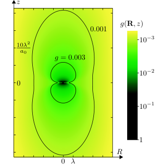
Increasing $R$ for $z<\lambda^{2}/a_{0}$, the Green’s function is dominated by the first term in Eq. (8) that describes a Gaussian with height $G(\mathbf{R}=\mathbf{0},z)\sim(a_{0}/z)\,G(\mathbf{0})$ and of width $R\sim\sqrt{a_{0}z}$; with decreasing $z$ this Gaussian peak becomes higher and narrows down to produce a dumbbell shape peak, see region I in the schematic Fig. 2 and the neck in the contour $g=0.003$ in Fig. 3. Increasing $R$ beyond $\sim\sqrt{a_{0}z}$, we enter region II in Fig. 2 where the second term in Eq. (8) dominates, interpolating smoothly between the peak and the non-dispersive result Eq. (7). This smooth interpolation through region II is of order $G(\mathbf{R},z)\sim(a_{0}/\lambda)^{2}G(\mathbf{0})$, with logarithmic corrections that become large at small values of $z$ where the narrow dumbbell peak at the origin decays more rapidly. Note that beyond the point $z\sim\lambda^{2}/a_{0}$ where the decay length $R\sim\sqrt{a_{0}z}$ meets the ellipsoidal shell, the Green’s function for $\mathbf{R}=\mathbf{0}$ already assumes a value $G(\mathbf{0},z\sim\lambda^{2}/a_{0})\sim(a_{0}^{2}/\lambda^{2})\,G(\mathbf{0})$ and no substantial variations with $R$ are seen within the region I.

Increasing instead the longitudinal distance $z$ at fixed $R<\lambda$, the Green’s function first remains flat (region II), then steeply increases $\propto e^{-\sqrt{\pi}R^{2}/a_{0}z}$ upon entering the peak region I at $z\sim\pm R^{2}/a_{0}$, and then decreases smoothly $\propto 1/z$, thus defining a maximum at $z\sim\pm R^{2}/a_{0}$. The resulting ridges located at the edges of the Gaussian peak are another manifestation of the dumbbell structure of the peak in $G(\mathbf{R},z)$, see Figs. 3 and 11.

The discussion has to be further refined in the regime of small $z\lesssim a_{0}$. As $z\to 0$, the first term in Eq. (8) diverges for $R=0$ and vanishes for $R>0$, formally approaching the 2D delta-function $\propto\delta^{2}(\mathbf{R}/a_{0})$. In reality, accounting for the $\mathbf{q}$-cutoff at the Brillouin zone boundary in Eq. (4) provides us with the finite result for the on-site Green’s function $G(\mathbf{R}=\mathbf{0},z=0)$. An expansion in the longitudinal direction for small $z\lesssim a_{0}$ then gives Koshelev

with the healing length $a_{h}\sim a_{0}[\ln(a_{0}/\xi)]^{1/2}$.

The decay length in the transverse direction at small $z$ is affected by the single-vortex elasticity that becomes relevant near the Brillouin zone boundary Blatter et al. 1994, Brandt 1977. Replacing the tilt modulus by $c_{44}(\mathbf{k})\to c_{44}(\mathbf{k})+(\varepsilon_{0}/a_{0}^{2})\ln(a_{0}/\xi)$ then entails a saturation of the decay scale $R\sim\sqrt{a_{0}z}$ in Eq. (8) at $R\sim a_{h}\sim a_{0}$ (we ignore a factor $\ln(a_{0}/\xi)$ in the scaling estimates) for $z\lesssim a_{0}$ (region III). For $R\gtrsim a_{h}$, we again cross over to the region II where the Green’s function assumes the constant value $\sim a_{0}^{2}/\lambda^{2}$, up to slow logarithmic corrections.

The above analysis has been carried out for a simplified diagonal expression $G_{\alpha\beta}=G\,\delta_{\alpha\beta}$. In a further step, one may replace the identity matrix $\delta_{\alpha\beta}$ by the full transverse projector $P_{\alpha\beta}^{\perp}(\mathbf{K})$, see Eq. (3). Focusing on the non-dispersive regime, the $\mathbf{q}$-integral in Eq. (6) picks up an additional angular dependence that depends on the geometry of the problem. For the component $G_{xx}$ evaluated in the $xz$-plane, we obtain the asymptotic dependence

where $\tilde{z}=(a_{0}/4\sqrt{\pi}\lambda)z$ is the scaled longitudinal length. The result (10) then exhibits a modified anisotropy at large distances: the simple scaling $G\propto 1/\sqrt{R^{2}+\tilde{z}^{2}}$ in the expression (7) is replaced with $G_{xx}\propto 1/2\tilde{z}$ when $\tilde{z}\gg R$ and $G_{xx}\propto 1/R$ at large $R\gg\tilde{z}$. Finally, while $G_{xy}=0$, we find that $G_{yy}(R,0,z)=(\tilde{z}/\sqrt{R^{2}+\tilde{z}^{2}})\,G_{xx}$. Note that $G_{xx}+G_{yy}=G$, as expected.

Having analyzed the elastic component in the pinning problem, we now turn to the discussion of the pinning potential $\varepsilon_{\mathrm{pin}}(\bm{\rho},\mathbf{u})$ in Eq. (1) for the cases of strong pinning, weak collective pinning, and the pinning by rare clusters. Note that the smallest transverse scale $R$ in the context of elasticity is the separation $a_{0}$ between vortices, while separations between defects as discussed below are considered small when $R$ reaches the effective size $\xi$ of defects. Hence, small lengths $R$ take a different meaning when talking about the vortex lattice (elasticity) or the pinning landscape.

We consider a lattice of flux lines or vortices aligned with the $z$-axis and described by the unperturbed vortex core positions $\mathbf{R}_{\mu}\in\mathbb{R}^{2}$. The pinning force acts on the vortex cores and the pinning energy can be expressed in the form [with ${\bm{\rho}=(\mathbf{R},z)]}$

with $\varepsilon_{\mathrm{pin}}^{\mu}[z,\mathbf{u}_{\mu}(z)]$ the random pinning potential acting on the $\mu$-th vortex line,

Here, $U_{\mathrm{pin}}(\mathbf{R},z)$ denotes the disorder potential generated by the material defects; assuming pinning due to point-like defects located at $\mathbf{r}_{i}=(\mathbf{R}_{i},z_{i})$, each with identical pinning energy $e_{p}$, the disorder potential takes the form

The factor $p(\mathbf{R})$ in Eq. (12) describes the vortex form factor, e.g., for a $\delta T_{c}$-type pinning mechanism Blatter et al. 1994, it reads $p(R)=1-|\psi(R)|^{2}$, with $\psi(R)$ the superconducting order parameter of the single-vortex solution to the Ginzburg-Landau equations. The simple Ansatz Schmid 1966, Clem 1975 $|\psi(R)|=R/(R^{2}+2\xi^{2})^{1/2}$ provides us with Lorentzian shape for the form factor, $p(R)=1/(1+R^{2}/2\xi^{2})$.

Combining Eqs. (12) and (13), we express the random pinning potential as

with $e_{p}(\mathbf{R})=-e_{p}\,p(\mathbf{R})$ the pinning potential due to a single defect; note that $e_{p}(\mathbf{R})$ is maximally negative for $\mathbf{R}=0$, i.e., pinning is maximal when the defect position $\mathbf{R}_{i}$ coincides with the perturbed vortex position $\mathbf{R}_{\mu}+\mathbf{u}_{\mu}(z)$. Substituting this result to Eqs. (2) and (11), we arrive at the equation for the displacement of the $\nu$-th vortex in the form

with the pinning force

acting in the direction transverse to the field. The last relation above applies for the Lorentzian-shaped potential.

In Eq. (15), we sum over all interactions between defects and vortices. In practice, we assume that no more than a single vortex can be pinned by an impurity and neglect interactions of vortices with defects far away from the vortex core, $|\mathbf{R}_{\mu}+\mathbf{u}_{\mu}(z_{i})-\mathbf{R}_{i}|\gg\xi$. The sum over the vortex index $\mu$ is then restricted to a single index $\mu(i)$ denoting the vortex closest to the impurity $i$. The relation (15) then allows to evaluate the displacement $\mathbf{u}_{\mu}(i)$ of the vortex $\mu$ pinned to the defect $i$ at the position $z_{i}$; this is nothing but the vortex tip displacement of the $\mu(i)$-th vortex,

The set of equations (17) represents a system of $N$ coupled non-linear equations for the displacements $\mathbf{u}_{i}$, with $N$ the total number of defects.

Within the strong pinning paradigm, we assume that defects act independently, allowing for a further simplification of Eq. (17) where the displacement $\mathbf{u}_{i}$ is ascribed exclusively to the action of the defect $i$; the summation over $j$ in Eq. (17) then reduces to the term $j=i$, i.e., we neglect the force exerted by distant defects $j\neq i$ on vortices $\mu(j)$ that contributes to the displacement $\mathbf{u}_{i}$ via the non-local Green’s function $G(\mathbf{R}_{\mu(i)}-\mathbf{R}_{\mu(j)},z_{i}-z_{j})$. It is exactly this simplification that will be dropped later on when considering strong pinning by pairs. The system of equations (17) then reduces to $N$ independent equations

with the effective vortex-lattice elasticity defined by $\bar{C}=1/G(\mathbf{0})$, see Eq. (5).

The resulting pinning-force density is obtained by summing the forces from all pinning sites. Note that the solution $\mathbf{u}_{i}$ in Eq. (18) depends only on the distance of the vortex from the pinning defect $\mathbf{x}_{i}=\mathbf{R}_{\mu(i)}-\mathbf{R}_{i}$. The average pinning force density is thus $\mathbf{F}_{\mathrm{pin}}=n_{p}\langle\mathbf{f}_{p}[\mathbf{x}+\mathbf{u}(\mathbf{x})]\rangle_{\mathbf{x}}$, where $n_{p}$ denotes the density of impurities and the average is taken with respect to the possible position vectors $\mathbf{x}$; assuming a uniform distribution of relative distances $\mathbf{x}$, the average then corresponds to a simple integration over $\mathbf{x}$.

It turns out that the pinning force can be expressed as the gradient of the total pinning energy, $\mathbf{f}_{p}[\mathbf{x}+\mathbf{u}(\mathbf{x})]=-\nabla_{\mathbf{x}}e_{\mathrm{pin}}(\mathbf{x})$, with $e_{\mathrm{pin}}(\mathbf{x})$ involving pinning and elastic terms,

If the solution $\mathbf{u}(\mathbf{x})$ to the on-site equation (18) is unique, implying a continuous evolution with $\mathbf{x}$, the average pinning force density vanishes, as follows from a simple integration of $\mathbf{f}_{p}[\mathbf{x}+\mathbf{u}(\mathbf{x})]$ over $\mathbf{x}$,

The single-defect Ansatz is thus meaningful only in the strong pinning regime where the solution for the on-site displacement is non-unique. In this case, different values (branches) for the total pinning energy $e_{\mathrm{pin}}(\mathbf{x})$ describe pinned and unpinned vortex states, see Fig. 4. Proper averaging accounts for the occupation of these branches which is unsymmetric, resulting in a non-vanishing average pinning-force density. We perform this analysis for a radially symmetric potential with a force $\mathbf{f}_{p}(\mathbf{r})=\hat{\mathbf{r}}f_{p}(r)$.

The condition for the appearance of multiple solutions is provided by the Labusch criterion Labusch 1969, Blatter et al. 2004, Brazovskii and Nattermann 2004

(we note that $\max f_{p}^{\prime}(r)=f_{p}^{\prime}(r_{m})$ with the inflection point $r_{m}$ obtained from $f_{p}^{\prime\prime}(r_{m})=0$). Furthermore, we assume that the vortices are driven in the positive $x$-direction and we parametrize their trajectories $\mathbf{x}=(x,b)$ through the longitudinal vortex position $x$ and an impact parameter $b$ in the transverse direction (the distinction between the ‘longitudinal’ field direction along $z$ and the ‘longitudinal’ direction of motion along $x$ should be clear from the context). The resulting pinning force averaged over positions $\mathbf{x}$ then points in the negative $x$-direction and is evaluated in two steps: first, we perform an averaging over $x$ at vanishing impact parameter $b=0$ and then we average over contributions from vortex trajectories with finite impact parameters $b\neq 0$.

For the case of a vanishing impact parameter $b=0$, Eq. (18) can be reduced to one dimension, $\bar{C}u=f_{p}(x+u)$ (we have dropped the index $i$). This is equivalent to minimizing the total pinning energy $e_{\mathrm{pin}}(x,u)=e_{p}(x+u)+\tfrac{1}{2}\bar{C}u^{2}$ with respect to $u$. Provided $x$ falls into the bistability region, $|x|\in[x_{\scriptscriptstyle-},x_{\scriptscriptstyle+}]$, there exist multiple solutions $u_{\mathrm{f}}(x)$, $u_{\mathrm{p}}(x)$ for the vortex tip displacement (denoting free and pinned vortex states) Blatter and Geshkenbein 2008, Willa et al. 2016, Thomann et al. 2017. Substituting these solutions to the total pinning energy provides multiple branches $e_{\mathrm{pin}}^{\mathrm{f},\mathrm{p}}(x)\equiv e_{\mathrm{pin}}[x,u_{\mathrm{f},\mathrm{p}}(x)]$, see Fig. 4. When going from large negative to large positive $x$, the branch occupation first undergoes a transition from the free to the pinned branch at the pinning point $-x_{\scriptscriptstyle-}$ and then another transition from the pinned to the free branch at the depinning point $x_{\scriptscriptstyle+}$. Averaging the pinning force $f_{p}[x+u_{o}(x)]$ over the occupied branches (as marked by the index $o\in\{\mathrm{f},\mathrm{p}\}$), the resulting integral over $x$ can be expressed as (see Eq. (20) and Thomann et al. 2017, Willa et al. 2016, Buchacek et al. 2019),

with the jumps in energy $\Delta e_{\mathrm{pin}}^{1}=[e_{\mathrm{pin}}^{\mathrm{f}}-e_{\mathrm{pin}}^{\mathrm{p}}]_{x=-x_{\scriptscriptstyle-}}$ and $\Delta e_{\mathrm{pin}}^{2}=[e_{\mathrm{pin}}^{\mathrm{p}}-e_{\mathrm{pin}}^{\mathrm{f}}]_{x=x_{\scriptscriptstyle+}}$ occurring at the pinning ($-x_{\scriptscriptstyle-}$) and depinning ($x_{\scriptscriptstyle+}$) points, respectively.

The result (22) remains unchanged even for a non-vanishing impact parameter $b\neq 0$ Thomann et al. 2017, Buchacek et al. 2019, provided the vortex passes the defect within the pinning distance $y_{p}$ along the $y$-direction; for the radially symmetric case, it turns out that $y_{p}=x_{\scriptscriptstyle-}$ and hence pinning occurs for impacts with $|b|<x_{\scriptscriptstyle-}$. For $|b|>x_{\scriptscriptstyle-}$, the pinning forces are small and multiple branches no longer exist, implying a vanishing average over $x$ Thomann et al. 2017, Buchacek et al. 2019. Finally, averaging the result (22) over $y$ contributes a factor $2x_{\scriptscriptstyle-}/a_{0}$ and thus

with $-\mathbf{e}_{x}$ denoting the unit vector pointing in the negative $x$-direction.

Eq. (23) assumes different scaling forms for the regime of very strong pinning $\kappa\gg 1$ and for moderately strong pinning $\kappa-1\ll 1$. In the first case, the jump sizes are related to the pinning potential depth via $\Delta e_{\mathrm{pin}}^{1}\sim e_{p}$ and $\Delta e_{\mathrm{pin}}^{2}\sim\kappa e_{p}$ Thomann et al. 2017, Buchacek et al. 2019, together providing the estimate for the magnitude of the position-averaged pinning force $\langle f_{p}\rangle_{\mathbf{x}}\sim(\kappa\xi^{2}/a_{0}^{2})\,f_{p}$ and a pinning force density

This result is interpreted as a pinning force $f_{p}\sim e_{p}/\xi$ [see Eq. (16)] due to a single defect exerted within the trapping area Ovchinnikov and Ivlev 1991, Blatter et al. 2004 $S_{\mathrm{trap}}=2y_{p}(x_{\scriptscriptstyle+}+x_{\scriptscriptstyle-})\sim\kappa\xi^{2}$; $S_{\mathrm{trap}}/a_{0}^{2}$ denotes the fraction of area occupied by trapped vortices.

For moderately strong pinning with $\kappa$ close to unity (that is particularly relevant for the pinning by rare events), the energy jumps are evaluated by expanding the pinning force around the inflection point at $r_{m}$, $f_{p}^{\prime\prime}(r_{m})=0$, where $f_{p}^{\prime}(r_{m})=\kappa\bar{C}$ is maximally positive Blatter et al. 2004, Koopmann et al. 2004, Buchacek et al. 2019, Willa et al. 2016,

In this situation, both jumps are identical and given by the expression Blatter et al. 2004, Buchacek et al. 2019 (note that $f_{p}^{\prime\prime\prime}(r_{m})<0$)

Using the scaling formulas $\bar{C}=f_{p}^{\prime}(r_{m})/\kappa\sim f_{p}\xi$ (provided $\kappa\sim\mathcal{O}(1)$), $f_{p}^{\prime\prime\prime}(r_{m})\sim f_{p}/\xi^{3}$ in Eq. (26) then gives

The pinning force density follows trivially,

and vanishes at the Labusch point $\kappa=1$, in accordance with the strong pinning criterion (21).

When pinning is weak, $\kappa<1$, individual defects fail to produce multi-valued solutions for the vortex displacement and the mean pinning force in Eq. (20) vanishes. Pinning then arises through the random action of defects within the collective pinning volume $V_{c}$ defined as the region where the spatial fluctuations of the vortex displacement $\langle u^{2}(\bm{\rho})\rangle=\langle[\mathbf{u}(\bm{\rho})-\mathbf{u}(\mathbf{0})]\rangle^{2}$ remains bounded by the pinning scale, $\langle u^{2}(\bm{\rho})\rangle\leq\xi^{2}$. The displacement correlation function can be systematically evaluated from Eq. (2) using the disorder-averaged correlator of the pinning energy density Eq. (11) Blatter et al. 1994, Larkin 1970,

with the correlation function $k(\mathbf{u}-\mathbf{u}^{\prime})=\int d^{2}\mathbf{R}\,p(\mathbf{R}-\mathbf{u})p(\mathbf{R}-\mathbf{u}^{\prime})$ related to the vortex form factor $p(R)$.

A qualitative estimate for the displacement correlator is provided by summing up distortions originating from all defects within a finite volume. In the vicinity of a reference defect characterized by the pinning force $f_{p}\sim e_{p}/\xi$, the distortion scale $u_{0}$ is given by the on-site Green’s function, $u_{0}\sim G(\mathbf{0})^{-1}f_{p}$. Expressing the on-site displacement through the effective vortex lattice stiffness $\bar{C}=G(\mathbf{0})^{-1}$ and estimating the Labusch parameter as $\kappa\sim f_{p}/\bar{C}\xi$ provides us with $u_{0}\sim\kappa\xi$. Assuming small defect densities and hence large typical inter-defect separations, the extension of the collective pinning volume falls into the non-dispersive regime of the Green’s function, see Eq. (7). Defects located a distance $\tilde{\rho}^{2}=R^{2}+(a_{0}^{2}/16\pi\lambda^{2})z^{2}$ away from the reference defect contribute with the displacement $u(\tilde{\rho})\sim u_{0}\>G(\tilde{\bm{\rho}})/G(\mathbf{0})\sim u_{0}(a_{0}^{2}/\lambda\tilde{\rho})$. Within the collective pinning volume $V_{c}=R_{c}^{2}L_{c}\sim(\lambda/a_{0})R_{c}^{3}$, these displacements add up with a random sign, as the forces from different defects are randomly directed; furthermore, only the fraction $\xi^{2}/a_{0}^{2}$ of defects that reside inside the vortex cores are directly attacking the vortices, resulting in a total squared displacement $\langle u^{2}(R_{c})\rangle\sim(\kappa\xi\,a_{0}^{2}/\lambda R_{c})^{2}(\xi^{2}/a_{0}^{2})\,n_{p}V_{c}$ on the scale $R_{c}$. Finally, the condition $\langle u^{2}(R_{c})\rangle\sim\xi^{2}$ provides us with the collective pinning radius

For small defect densities, as specified by the condition $\kappa^{2}n_{p}\xi^{2}a_{0}\ll 1$, the pinning radius $R_{c}\gg\lambda$ indeed falls into the non-dispersive regime (note that $\kappa\lesssim 1$). Finally, summing up the random force-contributions due to the active defects within the bundle volume $V_{c}=(\lambda/a_{0})R_{c}^{3}$, $F_{\mathrm{coll}}\sim[f_{p}^{2}n_{p}(\xi^{2}/a_{0}^{2})V_{c}]^{1/2}/V_{c}$, we find the collective pinning-force density

The collective pinning scenario described above sums up small competing contributions to the vortex lattice distortions arising from typical fluctuations in the defect distribution, involving defects that lie far away from each other within the collective pinning volume. However, it does not account for the presence of rare clusters, where two (or more) weak defects act cooperatively, giving rise to an effectively strong pinning center; the latter then is supposed to produce a distortion exceeding the scale $\xi$ of the pinning potential. In looking for promising candidate pairs, we consider Eqs. (7) and (8) that describe the decay of the Green’s function; these imply that the vortex displacement is substantially suppressed beyond a distance $\sim a_{0}$ away from the defect. Hence, two weak defects with $\tfrac{1}{2}<\kappa<1$ can be combined into a strongly-pinning object characterized by $\kappa>1$ and producing a displacement $u$ of order $\xi$ only if they are at most a longitudinal distance $z\sim a_{0}$ apart and pinning the same vortex core, i.e., they are separated by at most $R\sim\xi$ in the transverse dimension. This consideration then provides us with the density $(n_{p}a_{0}\xi^{2})\,n_{p}$ of strongly-pinning pairs. With only the fraction $\xi^{2}/a_{0}^{2}$ of those clusters being located within the vortex core area and each cluster exerting a pinning force $\sim f_{p}$, we arrive at the following estimate for the pinning force density due to defect pairs (with $1/2<\kappa<1$ still close to unity),

Assuming a magnetic field sufficiently above $H_{c1}$ such that $a_{0}<\lambda$, the pinning force due to such clusters dominates over the collective pinning contribution in Eq. (31) by a factor of $(\lambda/a_{0})^{2}$.

This factor in fact arises due to the dispersion of the tilt elastic modulus; in order to trace its origin, we need to understand the explicit dependence of the quantities contributing to both pinning mechanisms on the elastic properties of the vortex lattice, a dispersive tilt modulus $c_{44}(\mathbf{k})$ and non-dispersive shear modulus $c_{66}$. The collective pinning radius in Eq. (30) can be obtained by comparing the elastic energy $\mathcal{E}_{\mathrm{el}}(V_{c})\sim c_{66}(\xi/R_{c})^{2}V_{c}$ and the pinning energy $\mathcal{E}_{\mathrm{pin}}(V_{c})\sim[f_{p}^{2}n_{p}(\xi^{2}/a_{0}^{2})V_{c}]^{1/2}\xi$ accumulated within the pinning domain of volume $V_{c}=R_{c}^{2}L_{c}$. Assuming a large collective pinning volume where the dispersion of the tilt modulus is not relevant, the extensions $R_{c}$ and $L_{c}$ in the longitudinal and the transverse directions are related via $c_{66}(\xi/R_{c})^{2}\sim c_{44}(\mathbf{0})(\xi/L_{c})^{2}$, that provides us with (we write $c_{44}(\mathbf{0})=c_{44}$)

and the pinning force density is estimated as

We replace a factor $f_{p}^{3}$ in (34) with $\kappa^{3}(\bar{C}\xi)^{3}$,

and using $\kappa\sim 1$, $\bar{C}\sim a_{0}[c_{44}(K_{\rm\scriptscriptstyle BZ})c_{66}]^{1/2}$, and $[c_{44}(K_{\rm\scriptscriptstyle BZ})/c_{66}]^{1/2}\sim 1$, we obtain the desired result