High performance Wannier interpolation of Berry curvature and related quantities: WannierBerri code

The goal of this section is to introduce notation necessary for further discussion. For more details please refer to review Marzari et al. 2012 and original articles cited therein. The problem of Wannier interpolation is stated in the following way. First we evaluate the energies $E_{n{\bf q}}$ and wavefunctions $\psi_{n{\bf q}}({\bf r})\equiv e^{i{\bf q}\cdot{\bf r}}u_{n{\bf q}}({\bf r})$ from first principles on a rather coarse grid of $N_{\bf q}=N_{\bf q}^{1}\times N_{\bf q}^{2}\times N_{\bf q}^{3}$ wavevectors ${\bf q}$ within the reciprocal unit cell. Next we want to find the energies and wavefunctions at points on a denser grid of wavevectors ${\bf k}$. Further we will consistently use ${\bf q}$ and ${\bf k}$ to denote the ab initio and interpolation grids respectively.

For a group of entangled bands one can define a set of $J$ WFs defined as

where ${\cal J}_{\bf q}\geq J$ and ${\bf R}$ are real-space lattice vectors. The matrices $V_{mn^{\prime}}({\bf q})$ contain all the information of the construction of WFs, and may be generated by Wannier90 code. They are constrained by $\sum_{m=1}^{{\cal J}_{\bf q}}V^{*}_{mn}({\bf q})V_{mn^{\prime}}({\bf q})=\delta_{nn^{\prime}}$ and are chosen in such a way that the WFs are localized, which yields that the Bloch wavefunctions in the Wannier gauge

vary slowly with the ${\bf k}$ vector, unlike the true wavefunctions. Now let us see how WFs may be used to interpolate the band energies. First, one evaluates the matrix elements of the Hamiltonian

Next, to obtain energies at an arbitrary point ${\bf k}$ one needs to construct the Wannier Hamiltonian

which further may be diagonalized as

where $U_{nl^{\prime}}({\bf k})$ are unitary matrices with columns corresponding to the eigenvectors of the Hamiltonian (4). In a similar way, for any operator $\hat{X}$, for which the matrix elements are evaluated on the ab initio grid, one may obtain the real-space matrix elements

where in a simple case (e.g. $\hat{X}=\bm{\sigma}$)

or if $\hat{X}$ involves momentum-space derivatives, (e.g. the position operator $\hat{r}_{\alpha}\equiv i\partial/\partial k\alpha$) may also involve matrix elements between neighbouring ${\bf q}$ points (see Wang et al. 2006; Lopez et al. 2012 for details). Then the matrix elements may be interpolated to any ${\bf k}$ point in the Wannier gauge by

and further rotated to the Hamiltonian gauge

Note that equations (3), (4) are particular cases of (6) and (8). Equation (6) can be performed by means of FFT, and its result is periodic in ${\bf R}$ with a supercell formed by vectors $\mathbf{A}_{i}=\mathbf{a}_{i}N_{\bf q}^{i}$, where $\mathbf{a}_{i}$ ($i=1,2,3$) are the primitive unit cell vectors. Among the equivalent ${\bf R}$ vectors we choose those belonging to the corresponding Wigner-Seitz (WS) supercell. If an ${\bf R}$ vector belongs to the WS supercell boundary, we include all equivalent vectors on the boundary with the corresponding elements $X({\bf R})$ divided by the degeneracy of the ${\bf R}$ vector. Further, the MDRS method (see Sec. II.5) may also slightly modify the set of ${\bf R}$ vectors.

As an example, the total Berry curvature of the occupied manifold is interpolated Wang et al. 2006 via

where the ingredients of the equation are obtained using eqs. (8), (9) starting from $D_{nl,\alpha}\equiv\frac{\overline{H}_{nl,\alpha}^{\rm H}}{E_{l}-E_{n}}$, $H_{\alpha}^{\rm W}\equiv\partial_{\alpha}H^{\rm W}$, $A_{mn,\alpha}({\bf R})\equiv\langle\bm{0}m|\hat{r}_{\alpha}|{\bf R}n\rangle$, $\overline{\Omega}_{\gamma}^{\rm W}\equiv\epsilon_{\alpha\beta\gamma}\partial_{\alpha}A^{\rm W}_{\beta}$, $\partial_{\alpha}\equiv\partial/\partial{k_{\alpha}}$. The anomalous Hall conductivity is evaluated as an integral

Note, that while the direct Fourier transform (6) is performed only once for the calculation, and is not repeated for the multiple ${\bf k}$ points upon interpolation, the inverse Fourier transform (8) is repeated for every interpolation ${\bf k}$ point. And in fact it presents the most time-consuming part of the calculation involving Wannier interpolation as implemented in the Wannier90 code.

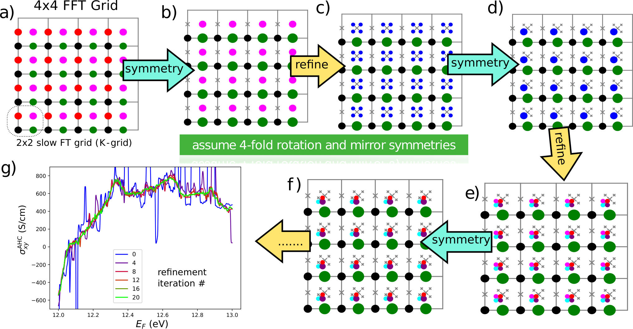
In this section we will see how the evaluation of (8) may be accelerated. It is easy to see that the computation time of a straightforward discrete Fourier transform scales with the number of ${\bf R}$ vectors and ${\bf k}$ points as $t\propto N_{\bf R}N_{\bf k}$, and we are typically interested in a case $N_{\bf k}\gg N_{\bf R}$ ($N_{\bf R}\approx N_{\bf q}$).

When the Fourier transform is done on a regular grid of ${\bf k}$ points, it is usually appealing to use the FFT. For that one needs to place the ${\bf R}$ vectors on a regular grid of size $N_{\bf k}$, fill the missing spots with zeros and perform the standard FFT, which will scale as $t\propto N_{\bf k}\log{N_{\bf k}}$. However there are some dificulties with such FFT. Mainly, because to perform FFT on a large grid implies storing the data for all ${\bf k}$ points in memory at the same time, which becomes a severe computational limitation. Also FFT does not allow to reduce computation to only the symmetry-irreducible ${\bf k}$ points, and is more difficult to do in parallel. However there is a way to combine the advantages of both the FFT and the usual discrete Fourier transform, leading to the concept of mixed Fourier transform.

We want to evaluate (8) for a set of ${\bf k}$ points.

where $0\leq n_{i}<N_{\bf k}^{i}$ – integers ($i=1,2,3$), $N_{\bf k}^{i}$ – size of interpolation grid, ${\bf b}_{i}$ — reciprocal lattice vectors. Now suppose we can factorize $N_{\bf k}^{i}=N_{\rm FFT}^{i}N_{\bf K}^{i}$ ²² 2 This is always possible unless $N_{\bf k}^{i}$ is a prime number. But for really dense grids, we can adjust $N_{\bf k}^{i}$ a bit, to be factorizable in any way we want. . Then the set of points (12) is equivalent to a set of points ${\bf k}={\bf K}+\bm{\kappa}$, where

where $0\leq l_{i}<N_{\bf K}^{i}$, $N_{\bf K}=\prod_{i}N_{\bf K}^{i}$, $0\leq m_{i}<N_{\rm FFT}^{i}$. This separation is illustrated in Fig 1(a), which shows a 2$\times$2 ${\bf K}$-grid, each corresponding to 4$\times$4 FFT grid (dots of a certain color). Now for each ${\bf K}$-point we can define

and then (8) reads as

The principle idea of mixed Fourier transform consists in performing the Fourier transform (15) as FFT, while (14) is performed directly. To perform the FFT we put all the ${\bf R}$ vectors on a grid $N_{\rm FFT}^{1}\times N_{\rm FFT}^{2}\times N_{\rm FFT}^{3}$, and a vector ${\bf R}=\sum_{i=1}^{3}n_{i}\mathbf{a}_{i}$ is placed on a slot with coordinates $\widetilde{n}_{i}=n_{i}\,{\rm mod}\,N_{\rm FFT}^{i}$ ($n_{i}$ are both positive and negative integers, while $0\leq\widetilde{n}_{i}<N_{\rm FFT}^{i}$). It is important to choose the FFT grid big enough, so that two different ${\bf R}$ vectors are not placed on the same slot in the grid.

The advantages of this approach are the following. First, the computational time scales as $t_{1}\propto N_{\bf K}N_{\bf R}$ for (14) and $t_{2}\propto N_{\bf K}N_{\rm FFT}\log N_{\rm FFT}$ for (15). Because it is required that $N_{\rm FFT}\geq N_{\bf R}$ (to fit all ${\bf R}$-vectors in the FFT box), we have $t_{1}\leq t_{2}\propto N_{\bf k}\log N_{\rm FFT}$ (in practice it occurs that $t_{1}\ll t_{2}$), which scales better then both the Fast and ’slow’ Fourier transforms. Next, we can perform Eqs. (14) and (15) independently for different ${\bf K}$-points. This saves us memory, and also offers a simple parallelization scheme. Also we can further restrict evaluation only to symmetry irreducible ${\bf K}$-points (Sec. II.3) and also perform adaptive refinement over ${\bf K}$-points (Sec. II.4).

Moreover, the evaluation time of a mixed Fourier transform only logarithmically depends on the size of the ab initio grid (recall that $N_{\rm FFT}\sim N_{\bf R}\sim N_{\bf q}$), while for the slow Fourier transform, the dependence is linear. However, in practice we will see (sec. IV) that the Fourier transform in the present implementation consumes only a small portion of computational time, and therefore the overall computational time is practically independent of the size of the ab initio grid.

When we integrate some quantity over the BZ, at every ${\bf K}$-point (after summing over $\bm{\kappa}$ points) we obtain the result as a rank-$m$ tensor $X_{i_{1},\ldots,i_{m}}({\bf K})$, for example the berry curvature vector $\Omega_{\gamma}$ or the conductivity tensor $\sigma_{xy}$. Then the BZ integral is expressed as a sum

and we initially set $\{{\bf K}\}$ as a regular grid (13a) and $w_{\bf K}=1/N_{\bf K}$. Suppose $G$ is the magnetic point group of the system ³³ 3 Because $X({\bf K})$ is invariant under translations, here we are interested in the point group, rather then space group.. We define the set of symmetry-irreducible ${\bf K}$ points $\rm irr$ as a a set of points that $\forall{\bf K},{\bf K}^{\prime}\in{\rm irr}$, $\forall g\in G$ holds $g{\bf K}\neq{\bf K}^{\prime}$, unless $g=E$ (identity). Then we can rewrite the sum (16) as

where we choose $g_{\bf K}$ such that $g_{\bf K}^{-1}{\bf K}\in{\rm irr}$ (this choice may be not unique), and obviously $g_{\bf K}=E$ for ${\bf K}\in{\rm irr}$. Thus, only the irreducible ${\bf K}$ points need to be evaluated. Next, to make sure that the result respects the symmetries, despite possible numerical inaccuracies, we symmetrize the result as:

Note, that ${\cal\widetilde{X}}={\cal X}$ if the model respects the symmetry precisely (e.g. when symmetry-adapted WFs Sakuma 2013 are used). Combining (17) and (18) and using $\sum_{f}^{G}f\cdot g_{\bf K}=\sum_{f}^{G}f$ we get

where $G\cdot{\bf K}$ denotes the orbit of ${\bf K}$ under action of group $G$. The latter equation reflects the implementation in the WB code. Starting from a regular grid of ${\bf K}$ points we search for pairs of symmetry-equivalent points. Whenever such a pair is found, one of the points is excluded and it’s weight is transferred to the other point. Compare Figs. 1(a) and (b): the red points are removed and their weight is moved to green points. Thus we end with a set of irreducible ${\bf K}$-point with weights $\widetilde{w}_{\bf K}=\sum_{{\bf K}^{\prime}}^{G\cdot{\bf K}}w_{{\bf K}^{\prime}}$. Next we evaluate $X({\bf K})$ (employing the corresponding interpolation scheme) only at symmetry-irreducible ${\bf K}$-points. Note, that although some ${\bf k}$-points corresponding to the same ${\bf K}$-point (same color in Fig. 1) are equivalent, we have to evaluate them all to be able to use the FFT. Finally, after summation, we symmetrize the result. The described procedure achieves two goals: (i) reduce the computational costs and (ii) make the result precisely symmetric, even if the WFs are not perfectly symmetric. In the present example we managed to obtain highly symmetric WFs (although without employment of symmetry-adapted WFs method), and therefore the symmetrization procedure does not change the result (within relative accuracy $\sim 10^{-5}$). However, for complex materials such quality of WFs is not always easy to achieve.

It is well known that in calculations of quantities involving Berry curvature or orbital moments, one performs integration over ${\bf k}$-space of a function that rapidly changes with ${\bf k}$. As a result, small areas of ${\bf k}$-space give the major contribution to the integral. Such areas often appear in the vicinity of Weyl points, nodal lines, as well as avoided crossings. To accelerate convergence with respect to the number of ${\bf k}$ points, we utilize adaptive mesh refinement similar to Refs. Yao et al. 2004; Wang et al. 2006. The authors of Yao et al. 2004; Wang et al. 2006 assumed a pre-defined threshold, and the ${\bf k}$-points yielding Berry curvature above the threshold were refined. This is inconvenient because one needs a good intuition to guess an optimal value for this threshold, because it depends both on the quantity one wants to calculate, and the material considered.

In WB it is implemented in a way that does not require initial guess from the user. This procedure, in combination with symmetrization described above, is illustrated in Fig. 1 in two dimensions (2D), while the actual work in 3D is described below. After excluding symmetry-equivalent ${\bf K}$-points (Fig. 1b) the results are evaluated for every ${\bf K}$ point and stored. We assume that initially each ${\bf K}$ point has weight $\widetilde{w}_{\bf K}$ and corresponds to a volume defined by vectors $\mathbf{c}_{\bf K}^{i}=\mathbf{b}_{i}/N_{\bf k}^{i}$ centered at ${\bf K}$. Then we pick a few ”most important ${\bf K}$-points”. The criteria of importance may be different - either the Maximal value for any $E_{F}$, or maximal value summed over all $E_{F}$, or yielding most variation over the $E_{F}$ (if the evaluated quantity is a function of Fermi level $E_{F}$). Suppose we selected the magenta point. Then those points are refined — replaced with 8 points around it with coordinates

where all combinationgs of $\pm$ signs are used. In Fig. 1c 4 new blue ${\bf K}$-points in the 2D case. The weight and volume of the initial point is distributed over the new points, thus $w_{{\bf K}^{\prime}}=\widetilde{w}_{\bf K}/8$ and $\mathbf{c}_{{\bf K}^{\prime}}^{i}=\mathbf{c}_{{\bf K}}^{i}/2$. Then the symmetrization is applied again (the four blue points are connected by 4-fold rotation) to exclude the equivalent points, and the weight of the equivalent points is collected on the remaining point, while the vectors $\mathbf{c}_{{\bf K}^{\prime}}^{i}$ are not changed. After the new ${\bf K}$-points are evaluated, we go to the next iteration of refinement. On each iteration any point may be refined, including both those from the initial regular grid, and those created during previous refinement iterations. The procedure stops after the pre-defined number of iterations was performed. Figure 1(g) shows how undesired artificial peaks of the the AHC curve are removed iteration by iteration, yielding a smooth curve (See sec. III for details).

The MDRS method Pizzi et al. 2020 allows to obtain a more accurate Wannier interpolation, in particular when moderate ${\bf q}$-grids are used in the ab initio calculations. With MDRS method the Fourier transform (8) is modified in the following way:

where $\mathbf{T}_{mn{\bf R}}^{(j)}$ are ${\cal N}_{mn{\bf R}}$ lattice vectors that minimise the distance $|{\bf r}_{m}-({\bf r}_{n}+{\bf R}+{\bf T})|$ for a given set $m,n,{\bf R}$. However, the evaluation of (21) is quite slower than (8), because every ${\bf k},m,n,{\bf R}$ an extra loop over $j$ is needed. Therefore calculations employing MDRS in postw90.x (which is enabled by default) takes more time. Instead it is convenient to re-define the modified real-space matrix elements as

only once for the calculation, and then the transformation to ${\bf k}$-space is performed via

Note, that the set of ${\bf R}$ vectors in (22) is increased compared to the initial set of vectors in (6) in order to fit all nonzero elements $\widetilde{X}_{mn}({\bf R})$ Equation (23) having essentially same form as (8), can be evaluated via mixed Fourier transform, as described in Sec. II.2.

Thus the MDRS method implemented in WB via Eqs. (22)-(23), and has practically no extra computational cost, while giving notable accuracy improvement.

It is often needed to study anomalous Hall conductivity (AHC) not only for the pristine Fermi level $E_{F}$, but considering it as a free parameter $\epsilon$. On the one hand it gives an estimate of the accuracy of the calculation, e.g. sharp spikes may indicate that the result is not converged. On the other hand $\epsilon$-dependence gives access to the question of the influence of doping and temperature, and also allows calculation of anomalous Nernst effect (27). As implemented in postw90.x, evaluation of multiple Fermi levels has a large computational cost. However there is a way to perform the computation of AHC for multiple Fermi levels without extra computational costs. To show this let’s rewrite (10), (11) as $\sigma_{\alpha\beta}(\epsilon)=-\epsilon_{\alpha\beta\gamma}\frac{e^{2}}{\hbar}\Omega_{\gamma}(\epsilon)$, where $\Omega_{\gamma}(\epsilon)=\sum_{\bf K}w_{\bf K}\Omega_{\gamma}({\bf K},\epsilon)$ and

where ${\bf k}={\bf K}+\bm{\kappa}$, the definitions of $P_{n}$ and $Q_{ln}$ straightly follow from (10), and we omit the cartesian index $\gamma$ further in this subsection. Now suppose we want to evaluate $\Omega(\epsilon_{i})$ for a series of Fermi levels $\epsilon_{i}$. For different ${\bf k}$-points and Fermi levels $\epsilon$ the sets of occupied $O({\bf k},\epsilon)$ and unoccupied states $U({\bf k},\epsilon)$ change and repeating this summations many times may be computationally heavy. Instead we note that when going from one Fermi level $\epsilon_{i}$ to another $\epsilon_{i+1}$ only a few states at a few $\bm{\kappa}$-points change from unoccupied to occupied. Let’s denote the set of such $\bm{\kappa}$-points as $\delta\kappa_{i}$ then, the change of the total Berry curvature is

where $\delta O_{i}({\bf k})\equiv O({\bf k},\epsilon_{i+1})-O({\bf k},\epsilon_{i})$. Note that if the step $\epsilon_{i+1}-\epsilon_{i}$ is small, then $\delta\kappa_{i}$ and $\delta O_{i}({\bf k})$ include only few elements, if not empty. Hence the evaluation of (25) will be very fast. Thus, the full summation (24) is needed only for the first Fermi level.

In a similar way this approach may be applied to orbital magnetization and other Fermi-sea properties. E.g. the orbital magnetization may be written as

where $C_{mn,\gamma}({\bf R})\equiv\epsilon_{\alpha\beta\gamma}\langle\bm{0}m|r_{\alpha}\cdot\hat{H}\cdot(r_{\beta}-R_{\beta})|{\bf R}n\rangle$, $B_{mn,\beta}({\bf R})\equiv\langle\bm{0}m|\hat{H}\cdot(r_{\beta}-R_{\beta})|{\bf R}n\rangle$ and the other ingredients were explained under (10). Equation (26) is written following the approach of Ref. Lopez et al. 2012, but the result has a different form, which can be straightforwardly processed by analogy with (24) and (25), where the first line of (26) expresses $P_{n}({\bf k})$ while the second and third lines correspond to $Q_{ln}({\bf k})$.

References

- Wannier (1937) G. H. Wannier, The structure of electronic excitation levels in insulating crystals, Phys. Rev. 52, 191 (1937).
- Marzari et al. (2012) N. Marzari, A. A. Mostofi, J. R. Yates, I. Souza, and D. Vanderbilt, Maximally localized Wannier functions: Theory and applications, Rev. Mod. Phys. 84, 1419 (2012).
- Vanderbilt and King-Smith (1993) D. Vanderbilt and R. D. King-Smith, Electric polarization as a bulk quantity and its relation to surface charge, Phys. Rev. B 48, 4442 (1993).
- King-Smith and Vanderbilt (1993) R. D. King-Smith and D. Vanderbilt, Theory of polarization of crystalline solids, Phys. Rev. B 47, 1651 (1993).
- Resta (1994) R. Resta, Macroscopic polarization in crystalline dielectrics: the geometric phase approach, Rev. Mod. Phys. 66, 899 (1994).
- Thonhauser et al. (2005) T. Thonhauser, D. Ceresoli, D. Vanderbilt, and R. Resta, Orbital magnetization in periodic insulators, Phys. Rev. Lett. 95, 137205 (2005).
- Ceresoli et al. (2006) D. Ceresoli, T. Thonhauser, D. Vanderbilt, and R. Resta, Orbital magnetization in crystalline solids: Multi-band insulators, chern insulators, and metals, Phys. Rev. B 74, 024408 (2006).
- Xiao et al. (2010) D. Xiao, M.-C. Chang, and Q. Niu, Berry phase effects on electronic properties, Rev. Mod. Phys. 82, 1959 (2010).
- Soluyanov and Vanderbilt (2011) A. A. Soluyanov and D. Vanderbilt, Computing topological invariants without inversion symmetry, Phys. Rev. B 83, 235401 (2011).
- Bradlyn et al. (2017) B. Bradlyn, L. Elcoro, J. Cano, M. G. Vergniory, Z. Wang, C. Felser, M. I. Aroyo, and B. A. Bernevig, Topological quantum chemistry, Nature 547, 298 (2017).
- Wu et al. (2018) Q. Wu, S. Zhang, H.-F. Song, M. Troyer, and A. A. Soluyanov, WannierTools: An open-source software package for novel topological materials, Computer Physics Communications 224, 405 (2018).
- Bouhon et al. (2019) A. Bouhon, A. M. Black-Schaffer, and R.-J. Slager, Wilson loop approach to fragile topology of split elementary band representations and topological crystalline insulators with time-reversal symmetry, Phys. Rev. B 100, 195135 (2019).
- Varnava et al. (2020) N. Varnava, I. Souza, and D. Vanderbilt, Axion coupling in the hybrid Wannier representation, Phys. Rev. B 101, 155130 (2020).
- Souza et al. (2001) I. Souza, N. Marzari, and D. Vanderbilt, Maximally localized Wannier functions for entangled energy bands, Phys. Rev. B 65, 035109 (2001).
- Slater and Koster (1954) J. C. Slater and G. F. Koster, Simplified lcao method for the periodic potential problem, Phys. Rev. 94, 1498 (1954).
- Gosálbez-Martínez et al. (2015) D. Gosálbez-Martínez, I. Souza, and D. Vanderbilt, Chiral degeneracies and Fermi-surface Chern numbers in bcc Fe, Phys. Rev. B 92, 085138 (2015).
- Wang et al. (2006) X. Wang, J. R. Yates, I. Souza, and D. Vanderbilt, Ab initio calculation of the anomalous Hall conductivity by Wannier interpolation, Phys. Rev. B 74, 195118 (2006).
- Lopez et al. (2012) M. G. Lopez, D. Vanderbilt, T. Thonhauser, and I. Souza, Wannier-based calculation of the orbital magnetization in crystals, Phys. Rev. B 85, 014435 (2012).
- Pizzi et al. (2014) G. Pizzi, D. Volja, B. Kozinsky, M. Fornari, and N. Marzari, BoltzWann: A code for the evaluation of thermoelectric and electronic transport properties with a maximally-localized Wannier functions basis, Computer Physics Communications 185, 422 (2014).
- Yates et al. (2007) J. R. Yates, X. Wang, D. Vanderbilt, and I. Souza, Spectral and fermi surface properties from Wannier interpolation, Phys. Rev. B 75, 195121 (2007).
- Ibañez Azpiroz et al. (2018) J. Ibañez Azpiroz, S. S. Tsirkin, and I. Souza, Ab initio calculation of the shift photocurrent by Wannier interpolation, Phys. Rev. B 97, 245143 (2018).
- Giustino et al. (2007) F. Giustino, M. L. Cohen, and S. G. Louie, Electron-phonon interaction using Wannier functions, Phys. Rev. B 76, 165108 (2007).
- Poncé et al. (2016) S. Poncé, E. Margine, C. Verdi, and F. Giustino, EPW: Electron–phonon coupling, transport and superconducting properties using maximally localized Wannier functions, Computer Physics Communications 209, 116 (2016).
- Tsirkin et al. (2018) S. S. Tsirkin, P. A. Puente, and I. Souza, Gyrotropic effects in trigonal tellurium studied from first principles, Phys. Rev. B 97, 035158 (2018).
- Qiao et al. (2018) J. Qiao, J. Zhou, Z. Yuan, and W. Zhao, Calculation of intrinsic spin Hall conductivity by Wannier interpolation, Phys. Rev. B 98, 214402 (2018).
- Ryoo et al. (2019) J. H. Ryoo, C.-H. Park, and I. Souza, Computation of intrinsic spin Hall conductivities from first principles using maximally localized Wannier functions, Phys. Rev. B 99, 235113 (2019).
- Marzari and Vanderbilt (1997) N. Marzari and D. Vanderbilt, Maximally localized generalized Wannier functions for composite energy bands, Phys. Rev. B 56, 12847 (1997).
- Mostofi et al. (2008) A. A. Mostofi, J. R. Yates, Y.-S. Lee, I. Souza, D. Vanderbilt, and N. Marzari, wannier90: A tool for obtaining maximally-localised Wannier functions, Computer Physics Communications 178, 685 (2008).
- Mostofi et al. (2014) A. A. Mostofi, J. R. Yates, G. Pizzi, Y.-S. Lee, I. Souza, D. Vanderbilt, and N. Marzari, An updated version of wannier90: A tool for obtaining maximally-localised Wannier functions, Computer Physics Communications 185, 2309 (2014).
- Pizzi et al. (2020) G. Pizzi, V. Vitale, R. Arita, S. Blügel, F. Freimuth, G. Géranton, M. Gibertini, D. Gresch, C. Johnson, T. Koretsune, J. Ibañez-Azpiroz, H. Lee, J.-M. Lihm, D. Marchand, A. Marrazzo, Y. Mokrousov, J. I. Mustafa, Y. Nohara, Y. Nomura, L. Paulatto, S. Poncé, T. Ponweiser, J. Qiao, F. Thöle, S. S. Tsirkin, M. Wierzbowska, N. Marzari, D. Vanderbilt, I. Souza, A. A. Mostofi, and J. R. Yates, Wannier90 as a community code: new features and applications, Journal of Physics: Condensed Matter 32, 165902 (2020).
- Mustafa et al. (2016) J. I. Mustafa, S. Coh, M. L. Cohen, and S. G. Louie, Automated construction of maximally localized Wannier functions for bands with nontrivial topology, Phys. Rev. B 94, 125151 (2016).
- Damle et al. (2015) A. Damle, L. Lin, and L. Ying, Compressed representation of kohn–sham orbitals via selected columns of the density matrix, Journal of Chemical Theory and Computation 11, 1463 (2015), pMID: 26574357, https://doi.org/10.1021/ct500985f .
- Damle and Lin (2018) A. Damle and L. Lin, Disentanglement via entanglement: A unified method for Wannier localization, Multiscale Modeling & Simulation 16, 1392 (2018), https://doi.org/10.1137/17M1129696 .
- Vitale et al. (2020) V. Vitale, G. Pizzi, A. Marrazzo, J. R. Yates, N. Marzari, and A. A. Mostofi, Automated high-throughput Wannierisation, npj Computational Materials 6, 66 (2020).
- Zhang et al. (2018) Z. Zhang, R.-W. Zhang, X. Li, K. Koepernik, Y. Yao, and H. Zhang, High-throughput screening and automated processing toward novel topological insulators, The Journal of Physical Chemistry Letters 9, 6224 (2018), https://doi.org/10.1021/acs.jpclett.8b02800 .
- Garrity and Choudhary (2020) K. F. Garrity and K. Choudhary, Database of Wannier tight-binding Hamiltonians using high-throughput density functional theory (2020), arXiv:2007.01205 [cond-mat.mtrl-sci] .
- (37) JARVIS-WannierTB database, https://www.ctcms.nist.gov/jarviswtb/.
- (38) WannierBerri code, https://wannier-berri.org/.
- (39) PyPI repository, https://pypi.org/project/wannierberri.
- git (a) WannierBerri git repository, https://github.com/stepan-tsirkin/wannier-berri (a).
- (41) During the work on the code and on the manuscript, the author did not receive any funding from Basque institutions or foundations. Usage of Basque language is motivated by a coincidental similarity to the Berry phase, and by good memories of the years that the author spent in the Basque region.
- Cooley and Tukey (1965) J. W. Cooley and J. W. Tukey, An algorithm for the machine computation of the complex Fourier series, Math. Computation 19, 297–301 (1965).
- Heideman et al. (1984) M. Heideman, D. Johnson, and C. Burrus, Gauss and the history of the fast Fourier transform, IEEE ASSP Magazine 1, 14 (1984).
- Duhamel and Vetterli (1990) P. Duhamel and M. Vetterli, Fast fourier transforms: A tutorial review and a state of the art, Signal Processing 19, 259 (1990).
- Van Loan (1992) C. Van Loan, Computational Frameworks for the Fast Fourier Transform (Society for Industrial and Applied Mathematics, USA, 1992).
- Yao et al. (2004) Y. Yao, L. Kleinman, A. H. MacDonald, J. Sinova, T. Jungwirth, D.-s. Wang, E. Wang, and Q. Niu, First principles calculation of anomalous Hall conductivity in ferromagnetic bcc Fe, Phys. Rev. Lett. 92, 037204 (2004).
- (47) This is always possible unless is a prime number. But for really dense grids, we can adjust a bit, to be factorizable in any way we want.
- (48) Because is invariant under translations, here we are interested in the point group, rather then space group.
- Sakuma (2013) R. Sakuma, Symmetry-adapted Wannier functions in the maximal localization procedure, Phys. Rev. B 87, 235109 (2013).
- Giannozzi et al. (2020) P. Giannozzi, O. Baseggio, P. Bonfà, D. Brunato, R. Car, I. Carnimeo, C. Cavazzoni, S. de Gironcoli, P. Delugas, F. Ferrari Ruffino, A. Ferretti, N. Marzari, I. Timrov, A. Urru, and S. Baroni, Quantum espresso toward the exascale, The Journal of Chemical Physics 152, 154105 (2020), https://doi.org/10.1063/5.0005082 .
- (51) Wannier90 code, http://www.wannier.org/.
- (52) The first is written by Wannier90, the other two by the interface of the ab initio code (e.g. pw2wannier90.x).
- (53) multiprocessing python module, https://pypi.org/project/multiprocessing.
- Destraz et al. (2020) D. Destraz, L. Das, S. S. Tsirkin, Y. Xu, T. Neupert, J. Chang, A. Schilling, A. G. Grushin, J. Kohlbrecher, L. Keller, P. Puphal, E. Pomjakushina, and J. S. White, Magnetism and anomalous transport in the Weyl semimetal PrAlGe: possible route to axial gauge fields, npj Quantum Materials 5, 5 (2020).
- Nagaosa et al. (2010) N. Nagaosa, J. Sinova, S. Onoda, A. H. MacDonald, and N. P. Ong, Anomalous Hall effect, Rev. Mod. Phys. 82, 1539 (2010).
- Xiao et al. (2006) D. Xiao, Y. Yao, Z. Fang, and Q. Niu, Berry-phase effect in anomalous thermoelectric transport, Phys. Rev. Lett. 97, 026603 (2006).
- Sodemann and Fu (2015) I. Sodemann and L. Fu, Quantum nonlinear Hall effect induced by Berry curvature dipole in time-reversal invariant materials, Phys. Rev. Lett. 115, 216806 (2015).
- Zhong et al. (2016) S. Zhong, J. E. Moore, and I. Souza, Gyrotropic magnetic effect and the magnetic moment on the Fermi surface, Phys. Rev. Lett. 116, 077201 (2016).
- Kawamura (2019) M. Kawamura, Fermisurfer: Fermi-surface viewer providing multiple representation schemes, Computer Physics Communications 239, 197 (2019).
- van Setten et al. (2018) M. van Setten, M. Giantomassi, E. Bousquet, M. Verstraete, D. Hamann, X. Gonze, and G.-M. Rignanese, The PseudoDojo: Training and grading a 85 element optimized norm-conserving pseudopotential table, Computer Physics Communications 226, 39 (2018).
- Hamann (2013) D. R. Hamann, Optimized norm-conserving Vanderbilt pseudopotentials, Phys. Rev. B 88, 085117 (2013).
- (62) VASP code, https://www.vasp.at/.
- Blöchl (1994) P. E. Blöchl, Projector augmented-wave method, Phys. Rev. B 50, 17953 (1994).
- Oliphant (2006) T. E. Oliphant, A guide to NumPy, Vol. 1 (Trelgol Publishing USA, 2006).
- Virtanen et al. (2020) P. Virtanen, R. Gommers, T. E. Oliphant, M. Haberland, T. Reddy, D. Cournapeau, E. Burovski, P. Peterson, W. Weckesser, J. Bright, S. J. van der Walt, M. Brett, J. Wilson, K. Jarrod Millman, N. Mayorov, A. R. J. Nelson, E. Jones, R. Kern, E. Larson, C. Carey, İ. Polat, Y. Feng, E. W. Moore, J. Vand erPlas, D. Laxalde, J. Perktold, R. Cimrman, I. Henriksen, E. A. Quintero, C. R. Harris, A. M. Archibald, A. H. Ribeiro, F. Pedregosa, P. van Mulbregt, and Contributors, SciPy 1.0: Fundamental Algorithms for Scientific Computing in Python, Nature Methods 17, 261 (2020).
- (66) pyFFTW python module, https://github.com/pyFFTW/pyFFTW.
- Frigo and Johnson (2005) M. Frigo and S. G. Johnson, The design and implementation of FFTW3, Proceedings of the IEEE 93, 216 (2005), special issue on “Program Generation, Optimization, and Platform Adaptation”.
- (68) lazy-property python module, https://pypi.org/project/lazy-property.
- git (b) Wannier90 git repository, https://github.com/wannier-developers/wannier90 (b).
- (70) QuantumEspresso code, https://www.quantum-espresso.org/.
- Hunter (2007) J. D. Hunter, Matplotlib: A 2d graphics environment, Computing in Science & Engineering 9, 90 (2007).
- (72) Inkscape vector graphics editor, https://inkscape.org.