Entanglement harvesting for Unruh-DeWitt detectors in circular motion
Abstract
We study the properties of the transition probability and entanglement harvesting phenomenon for circularly accelerated detectors locally interacting with massless scalar fields. The dependence of the transition probability on the parameters associated with the circular motion is first analyzed in detail. By a cross-comparison with the situation of the uniformly accelerated motion, we obtain that the transition probability and the possible thermalization behavior for detectors rotating with an extremely large circular radius are analogous to that for uniformly accelerated detectors, but for a very small linear speed and a large acceleration, the effective temperature which characterizes the detectors’ thermalization in a finite duration is much lower than that for uniformly accelerated detectors. We then focus on the phenomenon of entanglement harvesting in two special situations of circular trajectories, i.e., the coaxial rotation and the mutually perpendicular axial rotation by examining the concurrence as the entanglement measure in detail. We find that when two circularly accelerated detectors have equivalent acceleration and size of circular trajectory, the harvested entanglement rapidly decays with increasing acceleration or separation between two detectors. In contrast with the situation of uniform acceleration, the angular velocity would have significant impacts on entanglement harvesting. Especially for those detectors circularly moving in different directions, both the acceleration and trajectory radius play an important inhibiting role in entanglement harvesting. When two circularly accelerated detectors have different values of acceleration or angular velocity, we find that the entanglement can still be extracted by such detectors, even in the situation that one detector is at rest and the other is in a circular motion.
pacs
03.67.Bg,04.62.+v,03.65.Ud,03.67.-a,11.10.-zI Introduction
Quantum entanglement has been widely known as a key physical resource for performing some tasks in quantum information Plenio:1998; Horodecki:2001, and much progress has been made in understanding the features of entanglement in various aspects. For a two-atom system coupled with a common bath or environment, it has been found, in the framework of open quantum systems, that the generation of entanglement is likely to happen in certain circumstances Braun:2002; MSkim:2002; Schneider:2002; Basharov:2002; Jakobczyk:2002; Reznik:2003; Benatti:2003; Ficek:2003, and some other general entanglement dynamical behaviors such as the phenomenon of entanglement sudden death TYu:2004; Eberly:2007 or entanglement revival Ficek:2006 may also emerge. Recently, a more operational approach to studying quantum field entanglement has arisen from Valentini’s pioneer work Valentini:1991(and later revisited by Reznik Reznik:2003). It has been argued that a pair of initially uncorrelated atoms can become entangled via locally interacting with vacuum fields, even if they remain spacelike separated. Such proposed process has been extensively investigated in various circumstances involving the curved spacetime of a black hole Ver Steeg:2009; Olson:2011; BLHu:2012; Pozas-Kerstjens:2015; EDU:2016-1; EDU:2016-2; Pozas-Kerstjens:2016; Zhjl:2018; Zhjl:2019; Ng:2018; Ng:2018-2, which has now become recognized as the entanglement harvesting protocol Salton:2015. Since the entanglement harvesting phenomenon is sensitive to the curvature of spacetime, it may be used to discern the structure of spacetime EDU:2016-1 and distinguish a thermal background from the Hawking radiation background of an expanding universe Ver Steeg:2009.
On the other hand, the Unruh effect attests that accelerated detectors in Minkowski vacuum will observe a thermal radiation spectrum of particles Unruh:1976, which is closely related to the Hawking radiation, one of the most striking predications in quantum field theory in curved spacetime Birrell:1984. So, the Unruh effect is believed to offer a promising way to understanding other phenomena such as Hawking radiation of black holes and the thermal emission from cosmological horizons Birrell:1984; Crispino:2008. Nevertheless, a direct test of the Unruh effect would require some extreme physical conditions which are currently inaccessible in laboratory. However, a lot of effort has been made in exploring it through different means, including some novel proposals for experiments Crispino:2008 and other potentially measurable related quantum phenomena such as the geometric phase EDU:2011; Hu:2012; Zhjl:2016, the Lamb shift Audretsch :1995; Passante:1998; Rizzuto:2009; Zhu:2010, quantum entanglement Benatti:2004; Zhjl:2007; Landulfo:2009; Doukas:2010; Ostapchuk:2012; Hu:2015; Cheng:2018; Koga:2019; She:2019. More recently, it has been argued that there is a counter-intuitive phenomena (so-called anti-Unruh phenomena) that particle detectors can click less often or even cool down with the increase of the acceleration under certain conditions Brenna:2016; Garay:2016. Within certain parameter regime, the anti-Unruh effect may possibly be viewed as an amplification mechanism for quantum entanglement Li:2018.
Another interesting issue concerning the Unruh effect is the entanglement harvesting for accelerated detectors. It is worth noting that although this issue has recently been discussed in detail for the case of two linearly accelerated detectors in Refs. Salton:2015; Koga:2019, relatively little is known about entanglement harvesting for a pair of circularly accelerated detectors. Actually, as opposed to the situation of constant linear acceleration, the circular motion seems more interesting since it is easier to achieve, in a circular motion, the necessary large acceleration needed in the experimental verification of the Unruh effect Bell:1983. Recently, discussions on the entanglement dynamics of circularly accelerated atoms coupled with the electromagnetic vacuum have been performed in Ref. She:2019, but these results are limited to the Born-Markov approximation, requiring the pair of atoms have the same angular velocity and acceleration.
In this paper we will perform a more general study of the entanglement harvesting phenomenon of two circularly accelerated detectors, relaxing the limiting condition of the same angular velocity and acceleration. For simplicity, we will employ the well-known Unruh-DeWitt (UDW) model to depict the particle detector interacting with vacuum quantum fields DeWitt:1979. The paper is organized as follows. First, some basic formulae for the UDW detectors locally interacting with vacuum scalar fields are reviewed with the help of the entanglement harvesting protocol. In Sec. III, we will study the influence of the parameters concerned with the circular motion on the transition probability, such as the acceleration and circular trajectory radius. In addition, we also allow for a cross-comparison of the transition probabilities between the situation of circular acceleration and linear acceleration. In section IV, we will consider the entanglement harvesting phenomenon for a pair of circularly accelerating detectors along general circular trajectories, involving the coaxial and non-coaxial rotations. Some necessary numerical evaluation will be called for in the investigation. Finally, we conclude the paper with a summary in Sec.V. Throughout this paper the natural units are adopted for convenience.
II The basic formalism for entanglement harvesting protocol
In this section, we will introduce the description of a two-level atom interacting locally with a quantum scalar filed. We also review the derivation of basic formulas in entanglement harvesting protocol. Without loss of generality, two such atoms (labeled by and ) can be modeled with the UDW detectors. Now supposing that the spacetime trajectory of a detector is parameterized in terms of its proper time, then the interacting Hamiltonian for such a detector locally coupling with a real scalar field has the following form in the interaction picture
| (1) |
where is the coupling strength which is assume to be weak, is a Gaussian switching function controlling the duration of interaction via the parameter , and denote the ladder operators acting on the Hilbert space of the detector. Particularly, for a two-level atom system with an energy gap , we have and with and respectively denoting the ground and excited states. Here, the subscript specifies which UDW detector we are considering.
Suppose two such detectors and to be initially in their ground states, coupled with the scalar field in vacuum state , then the initial joint state can be written as . For simplicity, we assume that all detectors have an identical energy gap () and switching parameter () in their own rest frame. Governed by Hamiltonian Eq. (1), the composite system (two detectors plus the field) will undergo the unitary evolution with the corresponding operator satisfying
| (2) |
where denotes the time ordering operator. After some manipulations based on the perturbation theory, the finial state of the two detectors can be obtained by tracing out the field degrees of freedom EDU:2016-1; Zhjl:2018; Zhjl:2019
| (3) |
where the basis has been used. Here, the corresponding parameters in the reduced density matrix read
| (4) |
| (5) |
and
| (6) |
where is the Wightman function associated with the scalar field. In fact, denotes the probability that a detector has transitioned from its ground state to the excited state due to its interaction with the field EDU:2016-1, and represents the non-local correlations between two detectors Zhjl:2019.
According to the entanglement harvesting protocol Salton:2015, we can employ the concurrence as a measure of entanglement Wootters:1998, which can be evaluated straightforwardly from the -like density matrix given in Eq. (II) to yield the concurrence EDU:2016-1
| (7) |
Obviously, such entanglement measure is a competition between the non-local correlation and the transition probabilities, which in general is determined by the Wightman function of scalar fields. For the purpose of studying the entanglement harvesting phenomenon for circularly accelerated detectors, it is convenient to give the Wightman function and first examine the behavior of transition probabilities in the detector’s frame.
III The transition probabilities of circularly accelerated UDW detectors
In a 4-dimensional Minkowski spacetime, the Wightman function for massless scalar fields can be given in the popular “” representation Birrell:1984
| (8) |
The spacetime trajectory of circular motion can be parameterized by detector’s proper time She:2019; Doukas:2010; Kim:1987
| (9) |
where represents the radius of the circular trajectory in a plane parallel to -plane, is the angular velocity which can be either positive or negative in circular motion, and denotes the Lorentz factor. In the detector’s frame, the magnitude of acceleration satisfies , with the magnitude of linear velocity obeying . Note that , , and are not completely independent motion parameters, only two of them are actually independent. Substitute the trajectory (9) into Eq. (8), we can get the Wightman function
| (10) |
with .
As we can see from Eq. (10) that the corresponding Wightman function does not satisfy the Kubo-Martin-Schwinger (KMS) condition Kubo:1957; Martin:1959, i.e., we can not find a nonzero to ensure that the Wightman function obey the relation:
| (11) |
Therefore, for the circularly accelerated motion there is no well-defined KMS temperature in quantum field theory, which is quite different from the situation of a linearly uniformly accelerated detector with a KMS temperature proportional to the magnitude of acceleration Unruh:1976.
Substituting Eq. (10) into Eq. (4), we find that the transition probability (see Appendix A for detail)
| (12) |
where
| (13) |
and is the complementary error function, satisfying the identity . Although the first term in Eq. (12) is a regular integration, it is a messy task to get a simple analytical result and some numerical evaluations are needed Doukas:2010. However, for some certain extreme cases, approximate results can be obtained directly. For example, for an extremely large acceleration with high speed (i.e., and ), ( see Appendix B for more details), while for a small acceleration with high speed or extremely large radius (i.e., , ), through a saddle point approximation Nambu:2013, we can obtain ( see Appendix B)
| (14) |
Particularly, in the limit of , the first term of Eq. (12) is vanishing and the second term is just the transition probability of a rest detector with a Gaussian switching function, which is completely consistent with the result in Refs. EDU:2016-1; Nambu:2013.
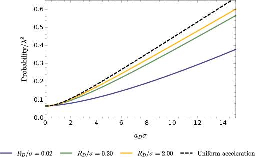
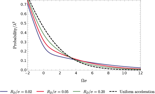
In order to understand how the transition probability depends on the acceleration and other parameters in circular motion, we illustrate the detailed behavior of the transition probability in Figs. (1-3). Here, throughout all the following plots the relevant physical quantities are adapted by the corresponding dimensionless ones in the unit of .

To allow for a cross-comparison of transition probabilities, here we have considered the following world line for a uniformly accelerated detector Birrell:1984; Crispino:2008; Rizzuto:2009; Salton:2015
| (15) |
where the magnitude of the linear constant acceleration is still denoted by . Similarly, the numerical evaluation of transition probabilities can also be carried out using Eq. (40) in Appendix A (for related discussions see Ref. Salton:2015). As shown in Fig. (1), the corresponding transition probability is a generally increasing function of acceleration irrespective of the circular or linear motion, and there does not seem to be anti-Unruh effect for the circularly accelerated detectors in Minkowski spacetime in terms of the transition probability. More interestingly, the transition probability for the linear uniform acceleration is more sensitive to the increasing acceleration, while for the circular motion, the smaller the trajectory radius is, the less variation the transition probability entails.
In Fig. (2), we explore the influence of the energy gap on the transition probability. It is easy to see that the transition probability is a monotonically decreasing function of . Especially for positive , corresponding to the initial ground state, the transition to excited state hardly happens for a big energy gap. This is consistent with our intuition that the larger the energy gap the harder the transition is to happen, which also follows straightforwardly from a mathematical examination of the general form of transition probability Eq. (12). It is worth pointing out that the larger the trajectory radius is, the faster the transition probability decays with increasing energy gap. These properties can be understood from the corresponding integrand in Eq. (12). For a fixed acceleration, is associated to the highly oscillatory part of Eq. (12). As the energy gap increases, a large trajectory radius will render the value of parameter much larger than 1, thus the integration part of Eq. (12) becomes vanishingly small as a result of the rapid oscillation of the cosine function.
To examine the influence of the circular trajectory radius on the transition probability, we plot the transition probability as a function of in Fig. (3). We find that the transition probability is a generally increasing function of the radius for a fixed , but the increased amount will be quite small as becomes large. It is worth pointing out that the limit of just corresponds to the situation of a rest point detector in Minkowski spacetime, and the transition probability is determined by the second term of Eq. (12) which is independent of the acceleration.
In order to get a better understanding of the possible thermalization process, it is convenient to define an effective temperature called by utilizing the excitation to de-excitation ratio (EDR) of the detector Fewster:2016, that is
| (16) |
where represents the EDR ratio. With the Gaussian switching function, the corresponding response function can be written in terms of the transition probability as
| (17) |
In general, the EDR temperature defined in Eq. (16) is complicated and dependent on the parameters , , . However, in the limit of an infinite interaction time and an extremely high speed (), the EDR temperature for circular acceleration is approximated to for (see Appendix B), which is higher than the EDR temperature for linear uniform acceleration Bell:1983.
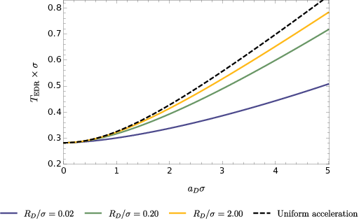
To illustrate the general thermalization process in a finite duration time, we have plotted how the EDR temperature depends on the acceleration at various trajectory radii in Fig. (4). It is easy to find that for a finite duration time the EDR temperature is an increasing function of acceleration, but the effective temperature for circular acceleration is lower than that for uniform acceleration when the energy gap is not too big, i.e., in comparison with circularly accelerated detectors, the uniformly accelerated detector would observe stronger thermal-like noise at the same magnitude of acceleration. Particularly, for a vanishingly small speed and a large acceleration with a not-extremely small energy gap(), the EDR temperature for circular motion, according to Eq. (12) and Eq. (16), approximately satisfies a simple relation: (see Appendix B), which is much lower than the EDR temperature for large linear uniform acceleration ().
IV Entanglement harvesting with UDW detectors in the circular motion
We now explore the entanglement harvesting phenomenon of two circularly accelerated detectors. For simplicity, we mainly focus on the spacetime trajectories of the detectors in two special cases: coaxial rotation and mutually perpendicular axial rotation (see Fig. (5)). Once having specified the trajectories, the concurrence can be calculated via the afore-given formulas.


IV.1 the situation of coaxial rotations
Suppose that detectors and with angular velocities and rotate around the -axis with the radii and . For the circular motion (9), the spacetime trajectories of the two detectors can be parameterized respectively by their proper times and
| (18) |
Here, and are corresponding Lorentz factors of detectors and respectively. The parameter is the separation between the two centers.
With the spacetime trajectories (IV.1), it is easy to find that the transition probabilities of the detectors can be straightforwardly calculated by using Eq. (12). The quantity representing the non-local correlations can be obtained by substituting Eq. (IV.1) and Eq. (8) into Eq. (II). For convenience, here we use to stand for in the case where the trajectories of two detectors are in parallel orbital planes described by Eq. (IV.1), thus result of can be generally written, after some algebraic manipulations, as
| (19) |
where the auxiliary functions read
| (20) |
| (21) |
When such two detectors are completely synchronously rotating around -axis, i.e., , Eq. (IV.1) can be further simplified to a one-dimensional integral
| (22) |
Due to the complexity of the integrand in Eq. (IV.1) and Eq. (IV.1), it is hard to obtain analytical results. Therefore, numerical evaluations are needed. Nevertheless, it is still quite a challenge to obtain numerical results since the integrand is a oscillatory function with singularities. Fortunately, the Wightman functions in fact are well-defined distributions EDU:2016-1; Bogolubov:1990. So, some techniques of a distribution function integral (in the Cauchy principal sense, see Appendix (A)) can be utilized to obtain the correct results, and some special numerical integration methods or strategies (e.g., composite Simpson’s rule and Legendre-Gauss quadrature) can be of help as well. Once the values of transition probabilities and are evaluated correctly, then the concurrence can be straightforwardly obtained from Eq. (7).
For simplicity, we first consider the impact of acceleration on entanglement harvesting in the situation where two detectors are rotating with the same acceleration and trajectory radius, i.e, (or equivalently, ). For such a situation, it is easy to judge that . Then the non-local correlation Eq. (IV.1) can be written as
| (23) |
If the two detectors are completely comoving (), then the double integral Eq. (IV.1) can be simplified further to a one-dimensional integral by integrating first
| (24) |


To facilitate a comparison with the situation of linear uniformly accelerated motion, we consider the following trajectory for uniform acceleration
| (25) |
where the symbol still denotes the magnitude of uniform acceleration and stands for the separation between two detectors. Similarly, the transition probabilities and the non-local correlations represented by can also be straightforwardly calculated by substituting the trajectories into Eq. (4) and Eq. (II) (the general expression for that uniform acceleration has been studied in Ref. Salton:2015).
In Fig. (6), the concurrence is plotted as a function of the separation in the unit of . As we will see that the entanglement (concurrence) in general is a fast decaying function of irrespective of the direction of angular velocity. It means that a large separation generally inhibits the detectors from harvesting entanglement. For , the entanglement harvested by circularly accelerated detectors is not expectedly sensitive to the trajectory radius, decaying a little more slowly than that for uniformly accelerated situation with increasing separation . However, for , the decaying behavior of entanglement will be more sensitive to the radius. Especially for a large radius (), it will rapidly fall to zero with increasing since the size of their circular trajectories can enlarge the average separation between two detectors.


In Fig. (7), the dependence of on the acceleration with various circular trajectory radii has been displayed. If such two detectors is in co-rotation with , it is easy to find that the larger the trajectory radius is, the faster the entanglement decays with the increasing acceleration . While if two detectors are in counter-rotation with an equal angular velocity (), a large radius renders the entanglement sharply decay with increasing acceleration, while a very small suppresses the decay as compared to the large radius case as increases, even making the entanglement decay much more slowly than that for the situation of uniform acceleration.
To understand the above referred characters, we recall that the concurrence is determined by the competition between the non-local correlation represented by and transition probabilities, which means that decreasing or increasing the transition probability may render the entanglement decrease. According to Eq. (IV.1), the non-local correlation is mainly dependent upon the average separation between two detectors, while the transition probability is dominantly determined by the value of acceleration as shown in Fig. (1). For the case of co-rotation (), the separation is always fixed, and the nearly uncharged value of and the increase of transition probability will make the concurrence monotonically decay over the entire range of . However, according to Fig. (1) and Fig. (4), we can see that a large trajectory radius would make the transition probability greater than that for a small radius, i.e., for not too small acceleration the detector rotating along with a larger circular trajectory may observe stronger thermal-like noise which can hinder it from harvesting entanglement. Thus, the larger the trajectory radius is, the faster the entanglement decays with the increasing acceleration. As for the case of counter-rotation (), if the trajectory radius is comparable with , the average separation between two detectors may increase during the finite duration time, which would make the non-local correlation decrease sharply. Then the sharply decreased and thermal-like noises render the harvested entanglement rapidly decay to zero as the acceleration increases. However, for a vanishingly small radius () in the counter-rotation situation, the decreased amount of is tiny due to the slight change of the separation between two detectors, hence the concurrence, analogous to the situation of co-rotation, will be governed by the value of the transition probability. Since the uniformly accelerated detectors observe stronger thermal-like noise for not too small acceleration (see Fig. (1) and Fig. (4)), then the entanglement harvested by circularly accelerated detectors would decay much more slowly than that by uniformly accelerated detectors. We also plot how the entanglement depends on the trajectory radius in Fig. (8) as a supplement. One may find that the trajectory radius would play an important inhibiting role in entanglement harvesting in the counter-rotation situation.
Now, let us turn to the question as to what happens to entanglement harvesting in the situation where the two detectors are coaxially rotating with different values of acceleration or angular velocity. For simplicity, we suppose that such two detectors are in concentric circular motion in -plane, i.e., , along the trajectory (IV.1). According to Eq. (IV.1), the corresponding concurrence can be straightforwardly obtained via numerical evaluations.


As shown in Fig.(9), it is difficult to extract the entanglement from the vacuum state of the quantum field throughout a large region of , irrespective of the direction of angular velocity. Most intriguingly, we find that is not zero but taking a finite value in the limit of (or equivalently, ). Such nonzero result at this special point tells us that the entanglement is likely to be still harvested by detectors and which are respectively at rest and in circular motion. In addition, it should be pointed out the harvested entanglement in the counter-rotation situation can approach its maximum at . Nevertheless, we expect that the peak value of entanglement for a fixed radius ratio should be achieved at the point of in the co-rotation situation.
In order to check this, and gain a better understanding of how the entanglement depends on the difference between the angular velocities of two detectors, we plot the concurrence as a function in Fig. (10). As we have seen that the smaller the radius difference between two detectors, the more the entanglement harvested. Remarkably, when two detectors are synchronously rotating (), the concurrence would certainly take the maximum value since the separation between two detectors always remains a minimum value, which is consistent with our intuitive perception that synchronously concentrically rotating detectors will extract the most entanglement from the vacuum state of a quantum field.
IV.2 the situation of mutually perpendicular rotation axes
Let us now consider that the two detectors are rotating in mutually perpendicular planes. The trajectories are given by
| (26) |
Note that the transition probabilities can still be obtained by carrying out Eq. (12) in numerical evaluation. Here, we use to denote in the case where the trajectories (IV.2) of two detectors are in mutually perpendicular orbital planes. Similarly, according to Eq. (II), the parameter can be written as
| (27) |
where
| (28) |
| (29) |
It is quite a challenge to further simplify the above expression of into a one-dimensional integral since the trajectories (IV.2) do not represent the comoving circular motion around a common rotating axis. However, it is easy to find that Eq. (IV.2) is independent of the direction of angular velocity in comparison with Eq. (IV.1). Thus, we can focus on the positive angular velocity for the trajectories Eq. (IV.2).


For the case where two circularly accelerated detectors have equivalent acceleration and trajectory radius, how the entanglement depends on the parameters of circular motion is illustrated in Figs. (11)-(13). Obviously, one can observe an analogous harvesting behavior that looks like the afore-studied situation of the coaxial rotation with equal and opposite angular velocities, though the quantitative details are different. For example, for a large trajectory radius, the harvested entanglement for perpendicular rotations falls to zero a little more slowly than that for coaxial rotations with opposite angular velocities (see the curves of in Fig. (6) and Fig. (11)). Similar conclusions can be obtained directly by comparing Fig. (7) with Fig. (12) or Fig. (8) with Fig. (13).


In Figs. (14)-(15), we have considered the situation of two detectors rotating at different accelerations or angular velocities along the trajectories (IV.2) with . When comparing Fig. (14) with Fig. (9)(the counter-rotation situation), similar results can be obtained: the larger the acceleration ratio between two detectors, the less the harvested entanglement. In the limit of (or ), will not be vanishing but take a non-zero maximum value. The most notable difference between Figs.(15) and (10) is that the peak of the extracted entanglement for non-coaxial rotations is localized at point rather than for coaxial rotations.
V conclusions
In this paper, we have performed detailed discussions on the properties of the transition probability of a circularly accelerated UDW detector coupled with the massless scalar fields with a Gaussian switching function, and investigated the entanglement harvesting phenomenon of two such detectors through the corresponding harvesting protocol. With the help of numerical evaluation, we have analyzed the influence of motion parameters on transition probabilities from various aspects. It was found that the transition probability of the circularly accelerated detector with a larger trajectory radius is more sensitive to the magnitude of acceleration, so is the effective temperature . By a cross-comparison of the situations of circularly and uniformly accelerated motion, we obtain that the transition probability and effective temperature for circularly accelerated detectors with an extremely large radius and that for uniformly accelerated detectors would behave analogously, but for a vanishingly small linear speed and a large acceleration with not-extremely small energy gap, in a finite duration, which differs from for uniformly highly accelerated detectors in a finite duration. And it seems that there are no anti-Unruh phenomena for circularly accelerated detectors interacting with the massless scalar fields in Minkowski spacetime.
For the purpose of well understanding the entanglement harvesting phenomenon, we focus on two special circular motion situations, i.e., coaxial rotation and mutually perpendicular axial rotation. When such two identical detectors are rotating along the circular trajectories with equivalent radius and acceleration, it was found that the harvested entanglement in both special circular motion situations decays with increasing acceleration or separation between two detectors. By a cross-comparison of the concurrence for circularly accelerated and uniformly accelerated detectors, we find that the trajectory radius and angular velocity in circular motion would have great effects on the entanglement harvesting phenomenon. Especially for two circularly accelerated detectors rotating in different directions, the trajectory radius would play an important inhibiting role in entanglement harvesting. In addition, it is worth pointing out that the behavior of entanglement generation for the situation of mutually perpendicular axes is analogous to that for the coaxial situation with , but the quantitative details are different slightly.
Finally, we have also investigated the entanglement harvesting for two identical detectors circularly rotating at different accelerations or angular velocities. The numerical results tell us that the entanglement harvesting still occurs in the quantum system composed of rest and circularly accelerated detectors. Particulary, in the situation of mutually perpendicular rotating axes (satisfying the circular orbit Eq. (IV.2)), the extracted entanglement will take the peak value when one detector is at rest and the other is circularly accelerated. Thus, an interesting question arises as to what the entanglement harvesting exactly behaves when two detectors are in completely different motion status. For example, one detector keeps at rest while the other is uniformly accelerated. Such a situation is analogous to that of one detector falling into black hole while the other stays outside. So, a further in-depth study on the entanglement harvesting for two detectors which are separated by a horizon in the Rindler spacetime or some curved spacetimes with a black hole is particularly desirable, which we would rather leave to a future work.
Acknowledgements.
This work was supported by the National Natural Science Foundation of China under Grant No.11690034.Appendix A Derivation of and
In this appendix we will derive the explicit form of the transition probability and from Eq. (4) and Eq. (II) respectively.
A.1 The transition probability
Recalling Eq. (4), and letting and , then the transition probability can be rewritten as
| (30) |
Inserting the Wightman function Eq. (10) into Eq. (A.1) and assuming lead to
| (31) |
with and . It is worth pointing out the integrand in the first term of Eq. (A.1) is a regular function, namely can be suppressed, while the second term can be calculated by using the technique of distribution functions. Let us pause to review some properties for distribution functions. Recall that the action of a distribution on a test function is defined by EDU:2016-1; Bogolubov:1990
| (32) |
which satisfies the following derivative relation
| (33) |
For the distribution , the action is defined as
| (34) |
where denotes the integral principle value. Then for the distribution , we can obtain Bogolubov:1990
| (35) |
According to the Sokhotski-Plemelj formula
| (36) |
the following identity can be obtained by differentiation
| (37) |
We can utilize the relation Eq. (33) to obtain the action of both the distributions and on a test function. In particular, for the distribution one has Bogolubov:1990
| (38) |
Now, let us return to the second integral of Eq. (A.1), we have
| (39) |
where we have used the identities Eqs. (35) and (38) in the last but one step. Thus, combining Eqs. (A.1) and (A.1) yields the transition probability given in Eq. (12).
Armed with the proposed technique of distribution functions, we can similarly get the expression of the transition probability for a uniformly accelerated detector with the trajectory (15), and the result is
| (40) |
where the superscript “” means the uniform acceleration situation.
A.2 The expression of
We begin from the definition of in Eq. (II), which can be rewritten as
| (41) |
where we have assumed in the last step. Therefore, the expression of can be straightforwardly obtained by substituting the Wightman function associated with the corresponding trajectory of two detectors into Eq. (41). In particular, if the Wightman function depends only on the difference between its two arguments (i.e., the Wightman function is only dependant on ), Eq. (41) can be further simplified into a one-dimensional integral via integrating first
| (42) |
Then it is straightforward to obtain Eq. (IV.1) and Eq. (24) by utilizing the explicit expression of the Wightman function.
Appendix B Some approximate results of and
To facilitate discussions on the possible thermalization process of circularly accelerated detectors, we here derive the expressions which are needed to approximately evaluate both the transition probability and the EDR temperature in some special cases.
B.1 approximate forms of
For convenience, the parameters and in Eq. (12) can be rewritten in terms of acceleration and the Lorentz factor , as
| (43) |
In the special case of an extremely large acceleration ( or ), it follows that . Then the Gaussian switching function can be simply dropped, therefore, it would be better to work from the first line of Eq. (A.1) rather than Eq. (12), then the transition probability takes a simple form
| (44) |
In principle, Eq. (44) can be performed by utilizing the residue theorem in the complex plane. However, the equation is not analytically solvable in the complex plane, therefore, the poles of the integrand in Eq. (44) can not be obtained exactly result. If both the speed and the energy gap are not vanishingly small ( is not small too, i.e., ), the pure imaginary poles of the integrand near would give the most important contribution to the integral. So we can expand the sine function to find the poles with the smallest imaginary part (such trackable treatment in details can also be found in Refs.Bell:1983; Audretsch :1995), leading to satisfying an approximate form , i.e.,
| (45) |
Thus, we can obtain the approximate form of via appropriate contour integration, and after some algebraic manipulation, Eq. (45) finally becomes
| (46) |
where represents the unit step function. Here, we have used the relation . Therefore, for an extremely large acceleration with high speed ( and ), Doukas:2010.
In the case of a small acceleration with high speed or extremely large radius ( , ), one may find that and for not too small energy gap. Then the first term in Eq. (12) can be written as
| (47) |
Eq. (B.1) can be approximately evaluated by the saddle point . With the help of the identity for a saddle point approximation at
| (48) |
we have
| (49) |
Here, we have used the relation , and so as to approximate the result.
Therefore, for , , the transition probabilities take following approximate form
| (50) |
B.2 approximate forms of
In the case of the infinitely long interaction time and high speed (,), the Gaussian switching functions can be ignored, the EDR temperature of circular acceleration can be obtained by substituting Eq. (46) into Eq. (16). In the assumption of , it is straightforward to get the EDR temperature . This result can also be obtained by straightforwardly calculating the transition probabilities per unit proper time Bell:1983; Audretsch :1995. Similarly, the EDR temperature for linear acceleration in the case of the infinitely long interaction time ( ) is exactly equal to Bell:1983; Audretsch :1995; Birrell:1984.
If the duration time is finite, for vanishingly small speed and large acceleration with a not-extremely small energy gap (), the integrand in the first term of Eq. (12) can be approximately written as
| (51) |
Because of and , Eq. (43) tells us that and . Thus, the vanishingly small and lead to
| (52) |
Assuming the energy gap is not-extremely small (), the second term in Eq. (12) can be approximately estimated as
| (53) |
Therefore, for a positive , we have
| (54) |
Substituting Eq. (54) into Eq. (16), and applying and , it is easy to get for circular acceleration.
Similarly, in regard to uniformly accelerated motion, the first term in Eq. (40) can be approximately evaluated, for an extremely large acceleration (), as
| (55) |
Therefore, for a positive ,
| (56) |
Thus, the EDR temperature for uniform acceleration can be expressed as
| (57) |
References
- (1) M. B. Plenio and V. Vedral, Contemp. Phys. 39, 431 (1998).
- (2) M. Horodecki, Quantum Inf. Comput. 1, 3 (2001).
- (3) D. Braun, Phys. Rev. Lett. 89, 277901 (2002).
- (4) M. S. Kim, J. Lee, D. Ahn, and P. L. Knight, Phys. Rev. A 65, 040101(R) (2002).
- (5) S. Schneider and G. J. Milburn, Phys. Rev. A 65,042107 (2002).
- (6) A. M. Basharov, J. Exp. Theor. Phys. 94, 1070 (2002).
- (7) L. Jakóbczyk, J. Phys. A 35, 6383 (2002).
- (8) B. Reznik, Found. Phys. 33, 167 (2003).
- (9) F. Benatti, R. Floreanini and M. Piani, Phys. Rev. Lett. 91, 070402 (2003).
- (10) Z. Ficek and R. Tanaś, J. Mod. Opt. 50, 2765 (2003).
- (11) T. Yu and J. H. Eberly, Phys. Rev. Lett. 93, 140404 (2004).
- (12) J. H. Eberly and T. Yu, Science 316,555 (2007).
- (13) Z. Ficek and R. Tanaś, Phys. Rev. A 74, 024304 (2006).
- (14) A. Valentini, Phys. Lett. A 153,321 (1991).
- (15) G.L. Ver Steeg and N.C. Menicucci, Phys. Rev. D 79, 044027 (2009).
- (16) S.J. Olson and T.C. Ralph, Phys. Rev. Lett. 106, 110404 (2011).
- (17) B.L. Hu, S.-Y. Lin and J. Louko, Class. Quant. Grav. 29, 224005 (2012).
- (18) A. Pozas-Kerstjens and E. Martín-Martínez, Phys. Rev. D 92,064042 (2015).
- (19) E. Martín-Martínez, A.R.H. Smith and D.R. Terno, Phys. Rev. D 93, 044001 (2016).
- (20) E. Martín-Martínez and B.C. Sanders, New J. Phys. 18, 043031 (2016).
- (21) A. Pozas-Kerstjens and E. Martín-Martínez, Phys. Rev.D 94, 064074 (2016).
- (22) L.J. Henderson, R.A. Hennigar, R.B. Mann, A.R.H. Smith and J. Zhang, Class. Quant. Grav. 35, 21LT02 (2018).
- (23) L.J. Henderson, R.A. Hennigar, R.B. Mann, A.R.H. Smith and J. Zhang, JHEP 05,178 (2019).
- (24) K. K. Ng, R. B. Mann, and E. Martín-Martínez, Phys. Rev. D 97, 125011 (2018).
- (25) K. K. Ng, R. B. Mann and E. Martín-Martínez, Phys. Rev. D 98,125005 (2018).
- (26) G. Salton, R. B. Mann, and N. C. Menicucci, New J. Phys.17,035001 (2015).
- (27) W. G. Unruh, Phys. Rev. D 14, 870 (1976).
- (28) N. D. Birrell and P. C. W. Davies, Quantum Fields in Curved Space, Cambridge Monographs on Mathematical Physics (Cambridge Univ. Press, Cambridge, UK, 1984).
- (29) L. C. B. Crispino, A. Higuchi, G. E. A. Matsas, Rev.Mod. Phys. 80, 787 (2008).
- (30) E. Martín-Martínez, I. Fuentes, Robert B. Mann, Phys. Rev. Lett. 107, 131301(2011).
- (31) J. Hu, H. Yu, Phys. Rev. A 85, 032105 (2012).
- (32) H. Zhai., J. Zhang and H. Yu, Ann. Phys. (N. Y.) 371, 338 (2016).
- (33) J. Audretsch and R. Müller, Phys. Rev. A 52, 629 (1995).
- (34) R. Passante, Phys.Rev. A 57,1590 (1998).
- (35) L. Rizzuto and S. Spagnolo, J. Phys.: Conf. Ser. 161, 012031 (2009).
- (36) Z. Zhu and H. Yu, Phys.Rev. A 82, 042108 (2010).
- (37) F. Benatti and R. Floreanini, Phys. Rev.A 70, 012112 (2004).
- (38) J. Zhang and H. Yu, Phys. Rev. D 75, 104014 (2007).
- (39) A. G. S. Landulfo and G. E. A. Matsas, Phys. Rev. A 80, 032315 (2009).
- (40) J. Doukas and B. Carson, Phys. Rev. A81, 062320 (2010).
- (41) D. C. M. Ostapchuk, S.-Y. Lin, R. B. Mann and B. L. Hu, JHEP 07, 072 (2012).
- (42) J. Hu and H. Yu, Phys.Rev. A 91, 012327 (2015).
- (43) S. Cheng, H. Yu, and J. Hu, Phys. Rev. D 98, 025001 (2018).
- (44) J. I. Koga, K. Maeda, G. Kimura, Phys. Rev. D 100, 065013 (2019).
- (45) J. She, J. Hu, H. Yu, Phys. Rev. D 99, 105009 (2019).
- (46) W. G. Brenna, R. B. Mann, and E. Martin-Martinez, Phys. Lett. B 757, 307 (2016).
- (47) L. J. Garay, E. Martin-Martinez, and J. de Ramon, Phys. Rev. D 94, 104048 (2016).
- (48) T. Li, B. Zhang, L. You, Phys.Rev.D 97, 045005 (2018).
- (49) J. S.Bell and J. M. Leinaas, Nucl. Phys. B 212, 131 (1983).
- (50) B. S. DeWitt, S. Hawking, and W. Israel, General Relativity: An Einstein Centenary Survey (Cambridge University Press Cambridge, 1979).
- (51) W. K. Wootters, Phys. Rev. Lett. 80, 2245 (1998).
- (52) S. K. Kim,K. S. Soh,J. H. Yee, Phys. Rev. D35,557 (1987).
- (53) R. Kubo, J. Phys. Soc. Jpn. 12, 570 (1957).
- (54) P. C. Martin and J. S. Schwinger, Phys. Rev. 115, 1342 (1959).
- (55) Y. Nambu, Entropy 15,1847-1874 (2013).
- (56) C. J. Fewster, B. A. Jurez-Aubry and J. Louko, Class.Quant. Grav. 33, 165003 (2016).
- (57) N. N. Bogolubov, A. A. Logunov, A. I. Oksak, and I. T. Todorov, General Principles of Quantum Field Theory (Springer, 1990).