Vis-MVSNet
Visibility-aware Multi-view Stereo Network
Abstract
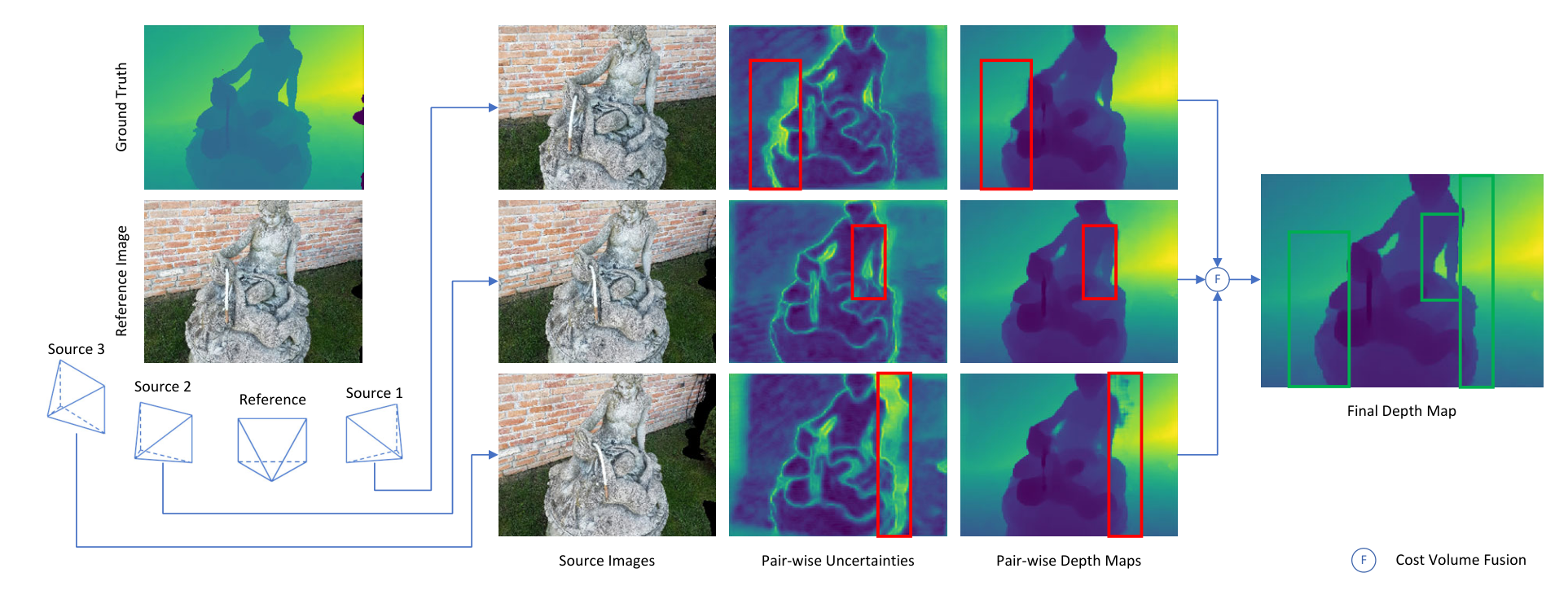
Learning-based multi-view stereo (MVS) methods have demonstrated promising results. However, very few existing networks explicitly take the pixel-wise visibility into consideration, resulting in erroneous cost aggregation from occluded pixels. In this paper, we explicitly infer and integrate the pixel-wise occlusion information in the MVS network via the matching uncertainty estimation. The pair-wise uncertainty map is jointly inferred with the pair-wise depth map, which is further used as weighting guidance during the multi-view cost volume fusion. As such, the adverse influence of occluded pixels is suppressed in the cost fusion. The proposed framework Vis-MVSNet significantly improves depth accuracies in reconstruction scenes with severe occlusion. Extensive experiments are performed on DTU, BlendedMVS, and Tanks and Temples datasets to justify the effectiveness of the proposed framework.
Hong Kong SAR, China ††affiliation: Everest Innovation Technology
Hong Kong SAR, China
1 Introduction
Multi-view Stereo (MVS) is one of the core problems in computer vision, which is essential to a variety of applications including image-based 3D modeling, city-scale survey and autonomous driving. While the problem is mainly solved by classical methods [Campbell et al.(2008)Campbell, Vogiatzis, Hernández, and Cipolla, Furukawa and Ponce(2009), Tola et al.(2012)Tola, Strecha, and Fua, Galliani et al.(2015)Galliani, Lasinger, and Schindler, Schönberger et al.(2016)Schönberger, Zheng, Frahm, and Pollefeys], recent learning-based methods [Yao et al.(2018)Yao, Luo, Li, Fang, and Quan, Yao et al.(2019)Yao, Luo, Li, Shen, Fang, and Quan, Gu et al.(2020)Gu, Fan, Zhu, Dai, Tan, and Tan] have also shown competitive results compared to previous state-of-the-arts. Learning-based methods usually extract deep image features from input images, which implicitly introduces global semantic such as specularity and reflection priors during the reconstruction process. Moreover, MVS networks usually apply 3D convolution neural networks (CNNs) for the cost volume regularization, which is more powerful than engineered cost regularization in classical methods.
One critical factor in MVS is the pixel-wise visibility: whether a 3D point is visible in given images. However, such visibility information is unknown before the 3D model is densely recovered, which implies a chicken-and-egg problem. In traditional MVS algorithms, the visibility issue is well understood: some approaches simply reject patch pairs according to pre-determined criteria, and then update the cost aggregation with only the inlier patch pairs [Furukawa and Ponce(2009), Tola et al.(2012)Tola, Strecha, and Fua, Xu and Tao(2019)]. More advanced approaches, such as COLMAP [Zheng et al.(2014)Zheng, Dunn, Jojic, and Frahm, Schönberger et al.(2016)Schönberger, Zheng, Frahm, and Pollefeys], compute the visibility information and aggregate the pair-wise matching cost based on a probabilistic framework, where visibility and depth are alternatively updated in E-step and M-step.
However, for current learning-based MVS methods, very few of them have acknowledged this problem and have explicitly handled the visibility issue. For example, MVSNet and its following works [Yao et al.(2018)Yao, Luo, Li, Fang, and Quan, Yao et al.(2019)Yao, Luo, Li, Shen, Fang, and Quan, Chen et al.(2019)Chen, Han, Xu, and Su, Gu et al.(2020)Gu, Fan, Zhu, Dai, Tan, and Tan, Cheng et al.(2020)Cheng, Xu, Zhu, Li, Li, Ramamoorthi, and Su, Yang et al.(2020)Yang, Mao, Alvarez, and Liu] feed multi-view features from all views into a variance-based cost metric regardless of the visibility of the pixel. Other methods apply either averaging [Hartmann et al.(2017)Hartmann, Galliani, Havlena, Van Gool, and Schindler] or max pooling [Huang et al.(2018)Huang, Matzen, Kopf, Ahuja, and Huang] to aggregate the matching cost. While it is possible that the network could implicitly learn how to discard the invisible views for each pixel, the unsolved visibility problem may inevitably deteriorate the final reconstruction.
In this work, we present an end-to-end network architecture that takes pixel-wise visibility information into account. The depth map is estimated from multi-view images in a two-step manner. First, matching is performed for each reference-source image pair and a latent volume representing the pair-wise matching quality is obtained. This volume further regresses to an intermediate estimation of a depth map and an uncertainty map, where the uncertainty is transformed from the depth-wise entropy of the probability volume. Second, to attenuate unmatchable pixels, we fuse all pair-wise latent volumes to one multi-view cost volume by using pair-wise matching uncertainties as weighting guidance. The fused volume is regularized and regresses to the final depth estimation. We also integrate several practical components from recent MVS networks, including group-wise correlation and [Guo et al.(2019)Guo, Yang, Yang, Wang, and Li] coarse-to-fine strategy [Gu et al.(2020)Gu, Fan, Zhu, Dai, Tan, and Tan] to further boost the overall reconstruction quality. Our network is end-to-end trainable and the uncertainty part is trained in an unsupervised manner. In this case, we can directly utilize existing MVS datasets with only ground truth depth maps to train the visibility-aware MVS network.
The proposed Vis-MVSNet is evaluated on DTU [Jensen et al.(2014)Jensen, Dahl, Vogiatzis, Tola, and Aanæs] and BlendedMVS [Yao et al.(2020)Yao, Luo, Li, Zhang, Ren, Zhou, Fang, and Quan] datasets and is benchmarked on Tanks and Temples [Knapitsch et al.(2017)Knapitsch, Park, Zhou, and Koltun] dataset. Our method ranks among all submissions in the Tanks and Temples online benchmark (until May 1, 2020). Comparisons with previous methods and ablation studies in the experiment section demonstrate the significant improvement bought by our approach, especially when the occlusion problem is severe in input images.
2 Related Work
Learning-based MVS
Learning-based methods have shown great potentials to replace each step in traditional MVS reconstructions. The learnable multi-view cost metric [Hartmann et al.(2017)Hartmann, Galliani, Havlena, Van Gool, and Schindler] is first proposed to measure the multi-view photo-consistency between image patches. Later, SurfaceNet [Ji et al.(2017)Ji, Gall, Zheng, Liu, and Fang] is proposed to learn the cost volume regularization from geometry ground truth. The authors of LSM [Kar et al.(2017)Kar, Häne, and Malik] apply the differentiable projection in the network and propose the first end-to-end learnable network for low-resolution MVS reconstruction. DeepMVS [Huang et al.(2018)Huang, Matzen, Kopf, Ahuja, and Huang] reprojects images to 3D plane-sweeping volumes, performs intra-volume aggregation, and applies inter-volume aggregation to fuse the volumes and generate the depth map output. RayNet [Paschalidou et al.(2018)Paschalidou, Ulusoy, Schmitt, Van Gool, and Geiger] encodes the camera projection to the network, and utilizes the Markov Random Field to predict the surface label.
Another recent popular network for MVS reconstruction is MVSNet [Yao et al.(2018)Yao, Luo, Li, Fang, and Quan]. MVSNet first extracts deep image features and then warps these features into the reference camera frustum to build a cost volume via differentiable homographies. To reduce the memory consumption during the network inference, the follow-up R-MVSNet [Yao et al.(2019)Yao, Luo, Li, Shen, Fang, and Quan] replaces the 3D CNNs regularization module with a 2D GRU recurrent network. Point-MVSNet [Chen et al.(2019)Chen, Han, Xu, and Su] proposes a point-based depth map refinement network to improve the output accuracy and MVS-CRF [Xue et al.(2019)Xue, Chen, Wan, Huang, Yu, Li, and Bao] introduces the conditional random field optimization during the depth map estimation. More recently, CasMVSNet [Gu et al.(2020)Gu, Fan, Zhu, Dai, Tan, and Tan], CVP-MVSNet [Yang et al.(2020)Yang, Mao, Alvarez, and Liu] and UCSNet [Cheng et al.(2020)Cheng, Xu, Zhu, Li, Li, Ramamoorthi, and Su] integrate the coarse-to-fine strategy to the learning-based MVS reconstruction. These works preserve an image feature pyramid and generate an initial depth estimation with large depth interval at a low resolution. In following stages, cost volumes are constructed with a narrow depth range centering at the depth estimation from previous stages. The coarse-to-fine architecture successfully reduces memory consumption so that they support deeper backbone networks and higher resolution outputs. However, these methods all apply a variance-based cost metric, which is under the assumption that a given pixel is visible in all input images. As a result, an increasing number of input images would lead to even a worse depth map estimation quality.
Visibility Estimation
Visibility estimation is a well-acknowledged problem in classic MVS reconstructions. Previous works include heuristic cost thresholding methods [Furukawa and Ponce(2009), Tola et al.(2012)Tola, Strecha, and Fua, Xu and Tao(2019)] and more complicated joint depth-visibility estimation methods [Zheng et al.(2014)Zheng, Dunn, Jojic, and Frahm, Schönberger et al.(2016)Schönberger, Zheng, Frahm, and Pollefeys]. For latter approaches, the per-pixel visibility is usually jointly recovered during the depth map estimation process through an EM-based method. However, these methods apply a probabilistic framework which is hard to be directly integrated with deep neural networks. To handle the visibility issue in the learning-based frameworks, we should consider other alternatives for joint depth map and visibility estimation.
Current deep learning methods take visibility into account in an implicit manner. MVSNet [Yao et al.(2018)Yao, Luo, Li, Fang, and Quan] reduces the feature volumes from different source views by variance metric which considers each view equally and claims that information from invisible pixels can be filtered out in the regularization. Such implicit method heavily relies on the regularization of the neural network. Besides, DeepMVS [Huang et al.(2018)Huang, Matzen, Kopf, Ahuja, and Huang] applies max pooling of multiple feature volumes to select the best latent representation, which is expected to be generated from a matchable pair. However, the fused volume is only related to the information from the best view, which loses the advantage of MVS that a more robust prediction can be produced by multiple observation. Instead, we start from pair-wise cost volumes to identify the pair-wise matching quality, and fuse the pair-wise volumes by weighted sum where weights of unmatchable pairs are reduced.
Uncertainty Estimation
In our approach, visibility is indicated by the matching uncertainty of the pair-wise depth map. Uncertainty (or confidence) estimation for two-view depth or disparity estimation has been widely studied for classic methods by Hu and Mordohai [Hu and Mordohai(2012)]. The majority of such methods examine the properties of the probability distribution over all the depth or disparity hypotheses. End-to-end deep neural networks [Poggi and Mattoccia(2016), Kim et al.(2018)Kim, Min, Kim, and Sohn, Tosi et al.(2018)Tosi, Poggi, Benincasa, and Mattoccia, Kim et al.(2019)Kim, Kim, Min, and Sohn] are also applied to estimate the uncertainty map for two-view stereo. Recently, Kendall and Gal [Kendall and Gal(2017)] propose to jointly estimate the network output and its uncertainty based on the Bayesian neural network. However, this method cannot be directly adopted in our framework because they operate on 2D outputs, while we believe that it is more reasonable to estimate uncertainty from the 3D probability volume. Therefore we follow [Zhang et al.(2020)Zhang, Yao, Luo, Li, Shen, Fang, and Quan] to use the depth-wise entropy of the probability volume to explicitly measure the pair-wise matching uncertainty.
3 Method
3.1 Overview
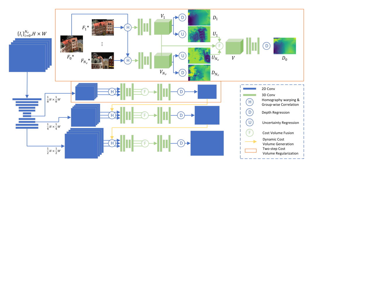
The outline of the framework is illustrated in Fig. 2. Given a reference image and a set of neighboring source images , the framework predicts a reference depth map aligned with . In our network, we apply the coarse-to-fine depth estimation strategy as recent networks [Gu et al.(2020)Gu, Fan, Zhu, Dai, Tan, and Tan]. First, all images are fed into a 2D UNet [Ronneberger et al.(2015)Ronneberger, Fischer, and Brox] which extracts the multi-scale image features. The extracted features at the last three scales in the decoder part are preserved and will be used to construct cost volumes at three different resolutions. For the reconstruction at the -th stage, the cost volume will be regularized and produce a depth map with the same resolution to the input feature map. Intermediate depth maps from previous stages will be used for the cost volume construction at next stages and will be served as the final output of the system.
The network details within the -th stage are described as follows. First, pair-wise cost volumes are constructed for each reference-source pairs. For the -th pair, by assuming that the reference image has depth , we can obtain a reprojected feature map from the source view. The groupwise correlation [Guo et al.(2019)Guo, Yang, Yang, Wang, and Li] between the reference and the warped source feature map is calculated as the cost map. Then the cost maps for all the depth hypothesis are stacked together as the cost volume. The resulting cost volume of the -th image pair in the -th stage is of size , where is the depth hypothesis number in the -th stage and is the group number of the group-wise correlation operation. The set of the hypotheses is predetermined for the first stage, and is dynamically determined for the second and third stages according to the depth map output of the previous stage. The calculation of the dynamic depth range will be explained in Sec. 3.4.
The regularization of the cost volume consists of two steps. First, every pair-wise cost volume is regularized to a latent volume separately. Then, all latent volumes are fused to which is further regularized to probability volume and regresses to the final depth map of the current stage via soft-argmax [Kendall et al.(2017)Kendall, Martirosyan, Dasgupta, Henry, Kennedy, Bachrach, and Bry] operation. The fusion of the latent volumes is visibility-awared. First, we measure the visibility by jointly inferring pair-wise depth and uncertainty. Each latent volume is transformed to a probability volume through additional 3D CNNs and the softmax operation. The depth map and the uncertainty map are jointly inferred via soft-argmax and entropy operation, which will be explained in Sec. 3.2. Then the uncertainty maps join the volume fusion as the weighting guidance, which is further described in Sec. 3.3.
3.2 Uncertainty Estimation
In current learning-based MVS, the depth map is usually regressed from probability volume via the soft-argmax operation. For simplicity, the stage number is omitted below. We denote the probability distribution over all the depth hypotheses as . The soft-argmax operation is equivalent to computing the expectation of this distribution and is computed as:
| (1) |
To jointly regress the depth estimation and its uncertainty, we assume that the depth estimation follows the Laplacian distribution [Kendall and Gal(2017)]. In this case, the estimated depth and the uncertainty maximize the likelihood of the observed ground truth: . Notice that the probability distribution also reflects the matching quality. We thus apply the entropy map of to measure the depth estimation quality. And the uncertainty map is transformed from by a function , which is presented as a shallow 2D CNN in the network.
| (2) |
The reason of adopting the entropy is that the randomness of the distribution is negatively related to the uni-modal distribution. And the uni-modality is an indicator of high confidence.
To jointly learn the depth map estimation and its uncertainty , we minimize the negative log likelihood described above.
| (3) |
Constants are omitted in the formula. For numerical stability, in practice we infer instead of directly. The log uncertainty map is also transformed from the entropy map by a shallow 2D CNN.
The loss can also be interpreted as applying attenuation to the loss between the estimation and the ground truth with a regularization term. The intuition is that the interference from the erroneous samples should be reduced.
3.3 Volume Fusion
In this section we introduce the visibility-aware volume fusion. For simplicity, the stage number is omitted. Given the pair-wise latent cost volumes , a single volume is fused from the volumes by weighted sum, where the weight is negatively related to the estimated pair-wise uncertainty.
| (4) |
The pixels with large uncertainty are more likely to be located in the occluded regions, and thus the values in the latent volume should be attenuated. The attenuation scale is chosen to be identical with the one in the joint loss (Eq. 3).
An alternative to the weighted sum is applying threshold for and perform a hard visibility selection for each pixel. However, lacking an interpretation of the value , we can only have an empirical threshold that may not be universal. Instead, the volumes are summed with normalized weight, which considers in a relative manner.
3.4 Coarse-to-fine Architecture
Our coarse-to-fine architecture mainly follows the recent Cas-MVSNet [Gu et al.(2020)Gu, Fan, Zhu, Dai, Tan, and Tan]. In all the stages, depth hypothesis are uniformly sampled from a depth range. The first stage takes image features at low resolution and constructs cost volume with the predetermined depth range but larger depth interval, while the following stages use high spatial resolution, narrower depth range and smaller depth interval.
For the first stage, the depth range is and the depth number is , where , and is predetermined. For the -th stage (), the depth range, sample number and interval are reduced. And the ranges are centered at the depth estimation from the previous stage, which are different for each pixels. The depth range for pixel is and the depth number is , where and are the predefined scaling factors, and is the final depth estimation of pixel from the last stage .
3.5 Training Loss
For each stage, the loss is the combination of the pair-wise loss, the pair-wise joint loss and the loss of the final depth map. And the total loss is the weighted sum of the loss from three stages. For all the losses derived from the absolute difference between the estimation and the ground truth, the per-pixel differences are divided by the depth interval of the final stage.
| (5) |
The pair-wise losses are included because the uncertainty loss tends to over-relax the pair-wise depth and uncertainty estimation. The pair-wise losses here could guarantee a qualified pair-wise depth map estimation.
 |
 |
 |
 |
| Family | Panther | Horse | Playground |
 |
 |
 |
 |
| Francis | Train | Lighthouse | M60 |
4 Experiment
4.1 Implementation
Training
Our network is trained on BlendedMVS [Yao et al.(2020)Yao, Luo, Li, Zhang, Ren, Zhou, Fang, and Quan] training set for most experiments (Sec. 4.2 and 4.4) and is trained on DTU training set [Jensen et al.(2014)Jensen, Dahl, Vogiatzis, Tola, and Aanæs] for DTU benchmarking (Sec. 4.3). For both training sets, we use the input image size of and output depth map size of . Source images for the given reference are selected as previous methods [Yao et al.(2018)Yao, Luo, Li, Fang, and Quan, Yao et al.(2019)Yao, Luo, Li, Shen, Fang, and Quan] and we set the number of source views to during training. For depth samples at different stages, we set the depth hypothesis numbers to , and depth range scaling factors respectively. The loss weights for each stage . The network is trained for 160k iterations with a batch size of 2 by an Adam [Kingma and Ba(2014)] optimizer. The initial learning rate is 0.001 and is halved at the 100k, 120k and 140k steps. All experiments are performed using one Nvidia GTX 1080Ti card.
Point cloud generation
Similar to previous works, we apply depth map filter and fusion approaches to merge all depth maps into a unified point cloud output. Both photometric and geometric consistencies are considered in our depth map filter and fusion step. For the photometric consistency, we follow [Yao et al.(2018)Yao, Luo, Li, Fang, and Quan] and generate probability maps to filter out unreliable pixels. The summation of probabilities of depth hypothesis within range are calculated as the probability map of a given depth map output. Moreover, in our coarse-to-fine architecture, we consider all probability maps at different stages, and the filtering criterion is that a pixel in a reference view will be preserved if and only if all probability maps from all three stages are higher than the corresponding thresholds . For geometric consistency, we preserve pixels whose depth estimation is consistent with the reprojected depth from at least views [Yao et al.(2018)Yao, Luo, Li, Fang, and Quan]. Finally, the median depth map fusion is applied to refine all depth maps. The 3D point cloud is obtained by projecting all refined depth maps into the 3D space.
| Tanks and Temples | DTU (mm) | |||||||||||
|---|---|---|---|---|---|---|---|---|---|---|---|---|
| Mean | Family | Francis | Horse | Lighthouse | M60 | Panther | Playground | Train | Acc. | Comp. | Overall | |
| COLMAP [Schönberger et al.(2016)Schönberger, Zheng, Frahm, and Pollefeys] | 42.14 | 50.41 | 22.25 | 25.63 | 56.43 | 44.83 | 46.97 | 48.53 | 42.04 | 0.400 | 0.664 | 0.532 |
| MVSNet [Yao et al.(2018)Yao, Luo, Li, Fang, and Quan] | 43.48 | 55.99 | 28.55 | 25.07 | 50.79 | 53.96 | 50.86 | 47.90 | 34.69 | 0.396 | 0.527 | 0.462 |
| Point-MVSNet [Chen et al.(2019)Chen, Han, Xu, and Su] | 48.27 | 61.79 | 41.15 | 34.20 | 50.79 | 51.97 | 50.85 | 52.38 | 43.06 | 0.342 | 0.411 | 0.376 |
| CVP-MVSNet [Yang et al.(2020)Yang, Mao, Alvarez, and Liu] | 54.03 | 76.50 | 47.74 | 36.34 | 55.12 | 57.28 | 54.28 | 57.43 | 47.54 | 0.296 | 0.406 | 0.351 |
| UCSNet [Cheng et al.(2020)Cheng, Xu, Zhu, Li, Li, Ramamoorthi, and Su] | 54.83 | 76.09 | 53.16 | 43.03 | 54.00 | 55.60 | 51.49 | 57.38 | 47.89 | 0.338 | 0.349 | 0.344 |
| CasMVSNet [Gu et al.(2020)Gu, Fan, Zhu, Dai, Tan, and Tan] | 56.84 | 76.37 | 58.45 | 46.26 | 55.81 | 56.11 | 54.06 | 58.18 | 49.51 | 0.325 | 0.385 | 0.355 |
| ACMM [Xu and Tao(2019)] | 57.27 | 69.24 | 51.45 | 46.97 | 63.20 | 55.07 | 57.64 | 60.08 | 54.48 | - | - | - |
| Vis-MVSNet | 60.03 | 77.40 | 60.23 | 47.07 | 63.44 | 62.21 | 57.28 | 60.54 | 52.07 | 0.369 | 0.361 | 0.365 |
4.2 Benchmarking on Tanks and Temples Dataset
We first evaluate our method on the intermediate set of Tanks and Temples dataset [Knapitsch et al.(2017)Knapitsch, Park, Zhou, and Koltun]. As mentioned in Sec. 4.1, we use the BlendedMVS training set [Yao et al.(2020)Yao, Luo, Li, Zhang, Ren, Zhou, Fang, and Quan] to train the network. BlendedMVS is a recent MVS dataset containing 113 indoor and outdoor scenes with 16904 MVS training samples in total. The dataset is split into 106 training scenes and 7 validation scenes. The trained model is directly applied to the Tanks and Temples benchmarking without fine-tuning.
We use an input image size of for reconstructions on the Tanks and Temples dataset. The source image number is set to for network inference and we choose , for depth map filter and fusion. Quantitative results are shown in Tab. 1 and corresponding point cloud reconstructions are illustrated in Fig. 3. Our Vis-MVSNet achieves a mean F-score of 60.03 and ranks among all the methods in the benchmark (until May 1, 2020), which outperforms all classical MVS methods [Schönberger et al.(2016)Schönberger, Zheng, Frahm, and Pollefeys, Xu and Tao(2019)] and recent learning-based approaches [Yao et al.(2018)Yao, Luo, Li, Fang, and Quan, Chen et al.(2019)Chen, Han, Xu, and Su, Yang et al.(2020)Yang, Mao, Alvarez, and Liu, Cheng et al.(2020)Cheng, Xu, Zhu, Li, Li, Ramamoorthi, and Su, Gu et al.(2020)Gu, Fan, Zhu, Dai, Tan, and Tan].
4.3 Benchmarking on DTU Dataset
The proposed method is also benchmarked on the DTU evaluation set [Jensen et al.(2014)Jensen, Dahl, Vogiatzis, Tola, and Aanæs]. DTU dataset contains 128 scans under fixed camera trajectories and 7 sets of lighting configuration. Every scan has 49 views with given camera parameters. As suggested by previous methods[Ji et al.(2017)Ji, Gall, Zheng, Liu, and Fang, Yao et al.(2018)Yao, Luo, Li, Fang, and Quan], DTU dataset is split into training set, validation set and evaluation set. Our model is trained on the DTU training set, which is mentioned in Sec. 4.1
For the depth map estimation, we use an input image size of and a fixed depth range of for all input images. The source image number is set to . We choose and for the depth map filter and fusion step. Quantitative results are shown in Tab. 1 and our method achieves a overall score of 0.365, which is comparable with other state-of-the-art methods.
| Setting | Fusion Method | Loss | ¡1 (%) | ¡3 (%) |
|---|---|---|---|---|
| base-var | Variance | 1.50 | 79.31 | 92.25 |
| base-ave | Average | 0.999 | 83.03 | 94.95 |
| base-max | Max Pooling | 0.956 | 84.71 | 95.19 |
| base-vis | Proposed | 0.908 | 85.35 | 95.48 |
| proposed | + Coarse-to-fine | 0.759 | 90.86 | 96.05 |
4.4 Ablation Study
In this section, we discuss other alternative volume fusion methods with implicit or explicit visibility awareness. To keep the simplicity of the network and clear demonstrate the effectiveness of the proposed component, we remove the coarse-to-fine architecture and directly use a MVSNet-like network as our baseline. The ablation study is performed on the BlendedMVS validation set and three types of evaluation metrics are considered: 1) the average L1 loss between the inferred depth map and the ground truth depth map; 2) the percentage of pixels with L1 error smaller than 1 depth-wise pixel ( percentage); and 3) the ¡3 percentage. Quantitative results are shown in Tab. 2 and Fig. 2
Baseline
In this setting (base-var), we directly use the variance metric to fuse the feature volumes into one cost volume. The base-var setting is widely adopted by MVSNet and its following works [Yao et al.(2018)Yao, Luo, Li, Fang, and Quan, Chen et al.(2019)Chen, Han, Xu, and Su, Yang et al.(2020)Yang, Mao, Alvarez, and Liu, Cheng et al.(2020)Cheng, Xu, Zhu, Li, Li, Ramamoorthi, and Su, Gu et al.(2020)Gu, Fan, Zhu, Dai, Tan, and Tan]. However, the variance operation is under the assumption that all pixels in the reference should be visible from all views. As a result, the increasing input image number would lead to even worse evaluation metrics (see Fig. 2)
Averaging
In this setting (base-ave), pair-wise cost volumes are fused to one multi-view volume by direct element-wise averaging. To fairly compare this setting with the proposed setting, we also apply the two step regularization as in the proposed framework. As is shown in Fig. 2, the ¡1 percentage accuracy of the base-ave is consistently increasing with the input image number. We believe the visibility information is implicitly encoded in the latent space and is dealt with by the two-step regularization. However, such implicit visibility awareness is apparently inferior to the proposed visibility fusion approach (see base-vis in Tab. 2 and Fig. 2).
Max Pooling
In this setting (base-max), the fused volume is obtained by finding the element-wise maximum of all the pair-wise volumes. This setting follows the fusion strategy of only considering the best matching pair among all reference-source image pairs. Similarly, all pair-wise losses are not counted toward the final loss. As is shown in Tab. 2 and Fig. 2, base-max outperforms base-ave but is still inferior to the proposed base-vis.
Weighted Averaging
This setting (base-vis) is the proposed Vis-MVSNet without the coarse-to-fine architecture. Compared with base-ave and base-max, this setting utilizes the intermediate uncertainty as the weighting guidance for the pair-wise volume fusion. As the result, the significance of invisible pixels will be explicitly reduced in the volume fusion step.
The quantitative comparison is shown in Tab. 2 and Fig. 2. A significant improvement can be observed after introducing the two step regularization to the baseline (base-ave and base-max v.s. base-var). In addition, the proposed fusion further improves the result (base-vis v.s. base-ave and base-max). Finally, the full model with coarse-to-fine architecture outperforms others by a significant margin (proposed v.s. others).
5 Conclusion
We have presented a visibility-aware depth inference framework for multi-view stereo reconstruction. We have proposed the two-step cost volume regularization, the joint inference of the pair-wise depth and the uncertainty, and the weighted average fusion of pair-wise volumes according to the uncertainty maps. The proposed method has been extensively evaluated on several datasets, demonstrating the effectiveness of the proposed visibility-aware depth inference framework.
6 Acknowledgments
This work is supported by Hong Kong RGC GRF 16206819 & 16203518 and T22-603/15N.
References
- [Campbell et al.(2008)Campbell, Vogiatzis, Hernández, and Cipolla] Neill DF Campbell, George Vogiatzis, Carlos Hernández, and Roberto Cipolla. Using multiple hypotheses to improve depth-maps for multi-view stereo. In European Conference on Computer Vision (ECCV), 2008.
- [Chen et al.(2019)Chen, Han, Xu, and Su] Rui Chen, Songfang Han, Jing Xu, and Hao Su. Point-based multi-view stereo network. In International Conference on Computer Vision (ICCV), 2019.
- [Cheng et al.(2020)Cheng, Xu, Zhu, Li, Li, Ramamoorthi, and Su] Shuo Cheng, Zexiang Xu, Shilin Zhu, Zhuwen Li, Li Erran Li, Ravi Ramamoorthi, and Hao Su. Deep stereo using adaptive thin volume representation with uncertainty awareness. In Computer Vision and Pattern Recognition (CVPR), 2020.
- [Furukawa and Ponce(2009)] Yasutaka Furukawa and Jean Ponce. Accurate, dense, and robust multiview stereopsis. IEEE transactions on pattern analysis and machine intelligence, 32(8):1362–1376, 2009.
- [Galliani et al.(2015)Galliani, Lasinger, and Schindler] Silvano Galliani, Katrin Lasinger, and Konrad Schindler. Massively parallel multiview stereopsis by surface normal diffusion. In International Conference on Computer Vision (ICCV), 2015.
- [Gu et al.(2020)Gu, Fan, Zhu, Dai, Tan, and Tan] Xiaodong Gu, Zhiwen Fan, Siyu Zhu, Zuozhuo Dai, Feitong Tan, and Ping Tan. Cascade cost volume for high-resolution multi-view stereo and stereo matching. In Computer Vision and Pattern Recognition (CVPR), 2020.
- [Guo et al.(2019)Guo, Yang, Yang, Wang, and Li] Xiaoyang Guo, Kai Yang, Wukui Yang, Xiaogang Wang, and Hongsheng Li. Group-wise correlation stereo network. In Computer Vision and Pattern Recognition (CVPR), 2019.
- [Hartmann et al.(2017)Hartmann, Galliani, Havlena, Van Gool, and Schindler] Wilfried Hartmann, Silvano Galliani, Michal Havlena, Luc Van Gool, and Konrad Schindler. Learned multi-patch similarity. In International Conference on Computer Vision (ICCV), 2017.
- [Hu and Mordohai(2012)] Xiaoyan Hu and Philippos Mordohai. A quantitative evaluation of confidence measures for stereo vision. IEEE transactions on pattern analysis and machine intelligence, 34(11):2121–2133, 2012.
- [Huang et al.(2018)Huang, Matzen, Kopf, Ahuja, and Huang] Po-Han Huang, Kevin Matzen, Johannes Kopf, Narendra Ahuja, and Jia-Bin Huang. Deepmvs: Learning multi-view stereopsis. In Computer Vision and Pattern Recognition (CVPR), 2018.
- [Jensen et al.(2014)Jensen, Dahl, Vogiatzis, Tola, and Aanæs] Rasmus Jensen, Anders Dahl, George Vogiatzis, Engil Tola, and Henrik Aanæs. Large scale multi-view stereopsis evaluation. In Computer Vision and Pattern Recognition (CVPR), 2014.
- [Ji et al.(2017)Ji, Gall, Zheng, Liu, and Fang] Mengqi Ji, Juergen Gall, Haitian Zheng, Yebin Liu, and Lu Fang. Surfacenet: An end-to-end 3d neural network for multiview stereopsis. In International Conference on Computer Vision (ICCV), 2017.
- [Kar et al.(2017)Kar, Häne, and Malik] Abhishek Kar, Christian Häne, and Jitendra Malik. Learning a multi-view stereo machine. In Advances in neural information processing systems, 2017.
- [Kendall and Gal(2017)] Alex Kendall and Yarin Gal. What uncertainties do we need in bayesian deep learning for computer vision? In Advances in neural information processing systems, 2017.
- [Kendall et al.(2017)Kendall, Martirosyan, Dasgupta, Henry, Kennedy, Bachrach, and Bry] Alex Kendall, Hayk Martirosyan, Saumitro Dasgupta, Peter Henry, Ryan Kennedy, Abraham Bachrach, and Adam Bry. End-to-end learning of geometry and context for deep stereo regression. In International Conference on Computer Vision (ICCV), 2017.
- [Kim et al.(2018)Kim, Min, Kim, and Sohn] Sunok Kim, Dongbo Min, Seungryong Kim, and Kwanghoon Sohn. Unified confidence estimation networks for robust stereo matching. IEEE Transactions on Image Processing, 28(3):1299–1313, 2018.
- [Kim et al.(2019)Kim, Kim, Min, and Sohn] Sunok Kim, Seungryong Kim, Dongbo Min, and Kwanghoon Sohn. Laf-net: Locally adaptive fusion networks for stereo confidence estimation. In Computer Vision and Pattern Recognition (CVPR), 2019.
- [Kingma and Ba(2014)] Diederik P Kingma and Jimmy Ba. Adam: A method for stochastic optimization. arXiv preprint arXiv:1412.6980, 2014.
- [Knapitsch et al.(2017)Knapitsch, Park, Zhou, and Koltun] Arno Knapitsch, Jaesik Park, Qian-Yi Zhou, and Vladlen Koltun. Tanks and temples: Benchmarking large-scale scene reconstruction. ACM Transactions on Graphics (ToG), 36(4):78, 2017.
- [Paschalidou et al.(2018)Paschalidou, Ulusoy, Schmitt, Van Gool, and Geiger] Despoina Paschalidou, Osman Ulusoy, Carolin Schmitt, Luc Van Gool, and Andreas Geiger. Raynet: Learning volumetric 3d reconstruction with ray potentials. In Computer Vision and Pattern Recognition (CVPR), 2018.
- [Poggi and Mattoccia(2016)] Matteo Poggi and Stefano Mattoccia. Learning from scratch a confidence measure. In British Machine Vision Conference (BMVC), 2016.
- [Ronneberger et al.(2015)Ronneberger, Fischer, and Brox] Olaf Ronneberger, Philipp Fischer, and Thomas Brox. U-net: Convolutional networks for biomedical image segmentation. In Medical image computing and computer-assisted intervention, 2015.
- [Schönberger et al.(2016)Schönberger, Zheng, Frahm, and Pollefeys] Johannes L Schönberger, Enliang Zheng, Jan-Michael Frahm, and Marc Pollefeys. Pixelwise view selection for unstructured multi-view stereo. In European Conference on Computer Vision (ECCV), 2016.
- [Tola et al.(2012)Tola, Strecha, and Fua] Engin Tola, Christoph Strecha, and Pascal Fua. Efficient large-scale multi-view stereo for ultra high-resolution image sets. Machine Vision and Applications, 23(5):903–920, 2012.
- [Tosi et al.(2018)Tosi, Poggi, Benincasa, and Mattoccia] Fabio Tosi, Matteo Poggi, Antonio Benincasa, and Stefano Mattoccia. Beyond local reasoning for stereo confidence estimation with deep learning. In European Conference on Computer Vision (ECCV), 2018.
- [Xu and Tao(2019)] Qingshan Xu and Wenbing Tao. Multi-scale geometric consistency guided multi-view stereo. In Computer Vision and Pattern Recognition (CVPR), 2019.
- [Xue et al.(2019)Xue, Chen, Wan, Huang, Yu, Li, and Bao] Youze Xue, Jiansheng Chen, Weitao Wan, Yiqing Huang, Cheng Yu, Tianpeng Li, and Jiayu Bao. Mvscrf: Learning multi-view stereo with conditional random fields. In International Conference on Computer Vision (ICCV), 2019.
- [Yang et al.(2020)Yang, Mao, Alvarez, and Liu] Jiayu Yang, Wei Mao, Jose M Alvarez, and Miaomiao Liu. Cost volume pyramid based depth inference for multi-view stereo. In Computer Vision and Pattern Recognition (CVPR), 2020.
- [Yao et al.(2018)Yao, Luo, Li, Fang, and Quan] Yao Yao, Zixin Luo, Shiwei Li, Tian Fang, and Long Quan. Mvsnet: Depth inference for unstructured multi-view stereo. In European Conference on Computer Vision (ECCV), 2018.
- [Yao et al.(2019)Yao, Luo, Li, Shen, Fang, and Quan] Yao Yao, Zixin Luo, Shiwei Li, Tianwei Shen, Tian Fang, and Long Quan. Recurrent mvsnet for high-resolution multi-view stereo depth inference. In Computer Vision and Pattern Recognition (CVPR), 2019.
- [Yao et al.(2020)Yao, Luo, Li, Zhang, Ren, Zhou, Fang, and Quan] Yao Yao, Zixin Luo, Shiwei Li, Jingyang Zhang, Yufan Ren, Lei Zhou, Tian Fang, and Long Quan. Blendedmvs: A large-scale dataset for generalized multi-view stereo networks. In Computer Vision and Pattern Recognition (CVPR), 2020.
- [Zhang et al.(2020)Zhang, Yao, Luo, Li, Shen, Fang, and Quan] Jingyang Zhang, Yao Yao, Zixin Luo, Shiwei Li, Tianwei Shen, Tian Fang, and Long Quan. Learning stereo matchability in disparity regression networks. arXiv preprint arXiv:2008.04800, 2020.
- [Zheng et al.(2014)Zheng, Dunn, Jojic, and Frahm] Enliang Zheng, Enrique Dunn, Vladimir Jojic, and Jan-Michael Frahm. Patchmatch based joint view selection and depthmap estimation. In Computer Vision and Pattern Recognition (CVPR), 2014.