Lax Connection and Conserved Quantities of Quadratic Mean Field Games

The integrability of quadratic MFG can be traced back to the Schrödinger representation Guéant 2012; Ullmo et al. 2019 of Eqs. (2)

$$\left\{\begin{aligned} &-\mu\sigma^{2}\partial_{t}\Phi=\frac{\mu\sigma^{4}}{2}\partial_{xx}\Phi+gm\Phi\\ &+\mu\sigma^{2}\partial_{t}\Gamma=\frac{\mu\sigma^{4}}{2}\partial_{xx}\Gamma+gm\Gamma\end{aligned}\right.\;,$$

(3)

obtained by performing a Cole-Hopf like transform

$$\left\{\begin{aligned} u(t,x)&=-\mu\sigma^{2}\log\Phi(t,x)\\ m(t,x)&=\Gamma(t,x)\Phi(t,x)\end{aligned}\right.\;.$$

(4)

NLS being integrable in the absence of external potential, we may expect that its MFG counterpart, equations (3), has the same property.

One of the most powerful methods when it comes to exploiting the integrability of MFG equation was first introduced by V. Zakharov and A. Shabat in their seminal paper of 1972 Shabat and Zakharov 1972. It presents what would later be known as the inverse scattering transform (IST) and constitutes the basis of soliton theory Novikov et al. 1984. This paper represents a first step in adapting this method, in its modern formulation, to MFG and relies heavily on the book by L. Faddeev and L. Takhtajan Faddeev and Takhtajan 2007. It presents the IST formalism and how it can be applied to MFG, but does not provide a solution to the system of equations (3). Instead it examines intermediate results, such as a way to generate first integrals of motion, and discusses some of the issues appearing in the context of MFG that will need to be addressed for further developments.

One of the more immediate benefits of this alternative representation is that it enables, in a fairly direct fashion, the introduction of various methods and notions originally developed to study and characterise problems of physics. Most notably, it brings forward the concepts of action and energy to the context of MFG. The system of Eqs. (3) can be obtained as stationarity conditions for an action functionnal $S$ defined as

$$S[\Gamma,\Phi]\equiv\int_{0}^{T}dt\int_{\mathbb{R}}dx\left[\frac{\mu\sigma^{2}}{2}(\Gamma\partial_{t}\Phi-\Phi\partial_{t}\Gamma)-\frac{\mu\sigma^{4}}{2}\partial_{x}\Gamma\partial_{x}\Phi+\frac{g}{2}(\Gamma\Phi)^{2}\right]\;,$$

(5)

so that

$$\mbox{ Eq.\penalty\ \eqref{intNLS}}\quad\Leftrightarrow\quad\left\{\begin{aligned} \frac{\delta S}{\delta\Phi}&=0\\ \frac{\delta S}{\delta\Gamma}&=0\end{aligned}\right.\;.$$

(6)

Existence of the action $S$ already implies, through Noether theorem, that conserved quantities are associated with the explicit symmetries of the problem, the most notable example being an Energy

$$\begin{aligned} E&=\int_{\mathbb{R}}dx\left[-\frac{\mu\sigma^{4}}{2}\partial_{x}\Gamma\partial_{x}\Phi+\frac{g}{2}\left(\Gamma\Phi\right)^{2}\right]\\ &=\int_{\mathbb{R}}dx\left[\frac{\sigma^{2}}{2}\left(\partial_{x}m\partial_{x}u+m\frac{(\partial_{x}u)^{2}}{\mu\sigma^{2}}\right)+\frac{g}{2}m^{2}\right]\end{aligned}\;,$$

(7)

which derives from the invariance of the action under a time translation:

$$m(x,t)\rightarrow m(x,t+t^{\prime})\quad\quad u(x,t)\rightarrow u(x,t+t^{\prime})\;.$$

(8)

Two other relevant conserved quantities with a clear physical meaning are the (normalized) number of players

$$N=\int_{\mathbb{R}}mdx=\int_{\mathbb{R}}\Phi\Gamma dx=1\;,$$

(9)

corresponding to $S$-invariance through a shift of the value function $u$ by a constant

$$u(x,t)\rightarrow u(x,t)+u^{\prime}\;,$$

(10)

and the momentum

$$P=\frac{1}{2}\int_{\mathbb{R}}(\Gamma\partial_{x}\Phi-\Phi\partial_{x}\Gamma)dx=-\frac{1}{2}\int_{\mathbb{R}}\left[\partial_{x}m+\frac{2m}{\mu\sigma^{2}}\partial_{x}u\right]dx\;,$$

(11)

associated with invariance under a space translation

$$m(x,t)\rightarrow m(x+x^{\prime},t)\quad\quad u(x,t)\rightarrow u(x+x^{\prime},t)\;,$$

(12)

under which the action $S$ is also invariant. The other conserved quantities exhibit more complicated expressions and their signification is usually more abstract. Relying on Noether theorem to find those is impractical, and we need a more systematic way of generating conserved quantities.

A technical discussion on the derivation of explicit expressions for the conserved quantities can be found in Section IV, using tools introduced in Section III. Hereafter, we provide a simple prescription for their construction, without demonstration.

For the sake of simplicity, we consider Mean Field Games with fields $\Phi$ and $\Gamma$ decreasing sufficiently fast at infinity

$$\left\{\begin{aligned} &\lim_{x\rightarrow{\pm}\infty}\Phi(x,t)=0\\ &\lim_{x\rightarrow{\pm}\infty}\Gamma(x,t)=0\end{aligned}\right.\quad\Rightarrow\quad\left\{\begin{aligned} &\lim_{x\rightarrow{\pm}\infty}u(x,t)=+\infty\\ &\lim_{x\rightarrow{\pm}\infty}m(x,t)=0\end{aligned}\right.\;.$$

(13)

As we shall show later, under this assumption every first integral of motion, denoted $Q_{n}$, can be written in the form

$$Q_{n}=\int_{\mathbb{R}}w_{n}\Phi dx=\int_{\mathbb{R}}\tilde{w}_{n}\Gamma dx\;,$$

(14)

where $\{w_{n}\}_{n\geq 0}$ and $\{\tilde{w}_{n}\}_{n\geq 0}$ are two families of polynomials in $\Phi$, $\Gamma$, and their derivatives, with first elements $w_{0}=\Gamma$ and $\tilde{w}_{0}=\Phi$, respectively, so that

$$Q_{0}=\int_{\mathbb{R}}\Gamma\Phi dx=N\;.$$

(15)

For every $n\geq 0$, the elements at order $n+1$ are defined recursively in terms of lower order ones

$$\left\{\begin{aligned} &w_{n+1}=\frac{\mu\sigma^{4}}{|g|}\left(-\partial_{x}w_{n}+\epsilon\,\Phi\,\sum_{k=0}^{n-1}w_{k}w_{n-k-1}\right)\\ &\tilde{w}_{n+1}=\frac{\mu\sigma^{4}}{|g|}\left(\partial_{x}\tilde{w}_{n}+\epsilon\,\Gamma\,\sum_{k=0}^{n-1}\tilde{w}_{k}\tilde{w}_{n-k-1}\right)\end{aligned}\right.\;.$$

(16)

where $\epsilon={\rm sgn}(g)$. It is easy to check that the first integrals of motion this procedure yields are the momentum $P$ (Eq. (11)) and the Energy $E$ (Eq. (7)) already obtained through Noether theorem

$$Q_{1}=\frac{1}{2}\int_{\mathbb{R}}(w_{1}\Phi+\tilde{w}_{1}\Gamma)dx=\frac{1}{2}\frac{\mu\sigma^{4}}{|g|}\int_{\mathbb{R}}(\Gamma\partial_{x}\Phi-\Phi\partial_{x}\Gamma)dx\;=\frac{\mu\sigma^{4}}{|g|}P\;,$$

(17)

and

$$Q_{2}=\frac{1}{2}\int_{\mathbb{R}}(w_{2}\Phi+\tilde{w}_{2}\Gamma)dx=\frac{\mu^{2}\sigma^{8}}{g^{2}}\int_{\mathbb{R}}dx\left[-\partial_{x}\Gamma\,\partial_{x}\Phi+\frac{g}{\mu\sigma^{4}}\,\left(\Gamma\Phi\right)^{2}\right]\;=2\frac{\mu\sigma^{4}}{g^{2}}E\;.$$

(18)

Next iterations allow to compute new, less obvious, conserved quantities such as

	$\displaystyle Q_{3}$	$\displaystyle=\frac{1}{2}\int_{\mathbb{R}}(w_{3}\Phi+\tilde{w}_{3}\Gamma)dx$		(19)
		$\displaystyle=\frac{1}{2}\frac{\mu^{3}\sigma^{12}}{|g|^{3}}\int_{\mathbb{R}}dx\left[\left(\Gamma\partial_{xxx}\Phi-\Phi\partial_{xxx}\Gamma\right)+3\,\frac{g}{\mu\sigma^{4}}\,\left(\Gamma^{2}(\partial_{x}\Phi)^{2}-\Phi^{2}(\partial_{x}\Gamma)^{2}\right)\right]\;,$

This new integral of motion is reminiscent of the generator of the modified KdV operator, which could be expected since mKdV and NLS are both part of the same AKNS hierarchy Ablowitz and Segur 1981. We may also compute easily the next integral

	$\displaystyle Q_{4}$	$\displaystyle=\frac{1}{2}\int_{\mathbb{R}}(w_{4}\Phi+\tilde{w}_{4}\Gamma)dx$		(20)
		$\displaystyle=\frac{\mu^{4}\sigma^{16}}{g^{4}}\int_{\mathbb{R}}dx\left[\partial_{xx}\Phi\partial_{xx}\Gamma-\frac{g}{\mu\sigma^{4}}\left(2\partial_{x}\Phi^{2}\partial_{x}\Gamma^{2}+\Phi^{2}(\partial_{x}\Gamma)^{2}+\Gamma^{2}(\partial_{x}\Phi)^{2}\right)+2\frac{g^{2}}{\mu^{2}\sigma^{8}}(\Phi\Gamma)^{3}\right]\;.$

As is often the case when dealing with non-linear PDEs, it will prove convenient to parametrize the system of equations (3) using dimensionless units.

In analogy with Bose-Einstein condensates, we introduced elsewhere Bonnemain et al. 2020b the healing length $\nu=\mu\sigma^{4}/\left|g\right|$ as a typical length scale of the problem. In a similar fashion, we can also define $\tau={2\mu^{2}\sigma^{6}}/{g^{2}}$ as a typical time scale. Denoting both $t^{\prime}={t}/{\tau}$ and $x^{\prime}={x}/{\nu}$ we can then write Eqs. (3) in a simpler form using dimensionless coordinates

$$\left\{\begin{aligned} &-\partial_{t^{\prime}}\Phi=+\partial_{x^{\prime}x^{\prime}}\Phi+2\,\epsilon\,\nu\,m\,\Phi\\ &+\partial_{t^{\prime}}\Gamma=+\partial_{x^{\prime}x^{\prime}}\Gamma+2\,\epsilon\,\nu\,m\,\Gamma\end{aligned}\right.\;,$$

(21)

where the value of $\epsilon=\pm 1$ is given by the sign of the interaction constant $g$. In this form, the healing length $\nu$ appears as the only relevant parameter.

The above representation (Eqs. (21) with all "primes" dropped) will be used for the rest of the paper. It will be especially useful when dealing with the several transformations required by the IST method.

The foundation of the IST method lies in the fact that Eqs. (21) can be seen as compatibility conditions for an auxiliary, overdetermined, linear system. Let $F=(f_{1},f_{2})$ be a vector function of $(x,t)$ defined by

$$\left\{\begin{aligned} &\partial_{x}F=U(x,t,\lambda)F\\ &\partial_{t}F=V(x,t,\lambda)F\\ \end{aligned}\right.\;,$$

(22)

where $U$ and $V$ are $2\times 2$ matrix functions depending on the space and time variables $x$ and $t$, but also on a spectral parameter $\lambda$, the importance of which will be made clear later. By Schwartz’s theorem, the two cross derivatives of $F$ have to be equal, which leads to the compatibility condition:

$$\partial_{t}U-\partial_{x}V+[U,V]=0\;,$$

(23)

and this relation has to hold no matter the value taken by $\lambda$. If we assume that

$$U=\kappa_{\epsilon}\begin{pmatrix}0&\Phi\\ \Gamma&0\end{pmatrix}+\begin{pmatrix}\frac{\lambda}{2}&0\\ 0&-\frac{\lambda}{2}\end{pmatrix}\;,$$

(24)

with $\epsilon=\pm 1$ as in (21) and, respectively, $\kappa_{-}=\sqrt{\nu}$ and $\kappa_{+}=i\sqrt{\nu}$, and

$$V=\kappa_{\epsilon}\begin{pmatrix}\kappa_{\epsilon}\Phi\Gamma&-\partial_{x}\Phi\\ \partial_{x}\Gamma&-\kappa_{\epsilon}\Phi\Gamma\end{pmatrix}-\lambda U\;,$$

(25)

then, under the constraints Eqs. (13), Eqs. (21) are equivalent to the compatibility condition (23). More general boundary conditions can be accounted for by modifying $V$ (see for instance the chapter The case of finite density in Faddeev and Takhtajan 2007). What this representation brings is a fairly natural geometric interpretation. The matrices $U$ and $V$ can be seen as the $x$ and $t$ components of a connection (or gauge field) in the vector bundle $\mathbb{R}^{2}\times\mathbb{R}^{+2}$, while the left hand side of compatibility condition (23) can be seen as the curvature (or strength field) of this connection according to the Ambrose-Singer theorem Ambrose and Singer 1953. Hence the name zero-curvature representation. In the field of classical integrable systems this is known as Lax connection and the compatibility equation (23) is equivalent to Lax equation in the limit of an infinite number of degrees of freedom Babelon et al. 2003.

A reasonable progression, once we interpret $(U,V)$ as a connection, is to consider the parallel transport it induces. Let $\gamma$ be a curve in $\mathbb{R}^{2}$ and $\gamma_{1}...\gamma_{N}$ a partition into $N$ adjacent segments. We define the parallel transport along $\gamma$ as

$$\Omega_{\gamma}=\lim_{N\rightarrow\infty}\left[\mathcal{P}\prod_{n=1}^{N}\left(\mathbb{1}+\int_{\gamma_{n}}(Udx+Vdt)\right)\right]\;,$$

(26)

where $\mathcal{P}$ denotes path ordering and $\mathbb{1}$ the $2\times 2$ identity matrix. A more compact notation for this expression would be

$$\Omega_{\gamma}=\mathcal{P}\exp\int_{\gamma}(Udx+Vdt)\;.$$

(27)

This last expression is also particularly convenient for two reasons. The first one is that it makes it clear that if $\gamma$ represents a path from some point $(x,s)$ to some other point $(y,t)$, and given the initial data $F(x,s)$, the solution of equations (22) can be written as a covariantly constant vector field

$$F(y,t)=\Omega_{\gamma}F(x,s)\;.$$

(28)

The second, and maybe more important, reason is that it shows clearly that parallel transport over any closed curve $\gamma_{0}$ (holonomy of the connection) is trivial by way of the non-Abelian Stokes theorem (cf appendix A). Indeed, thanks to the vanishing of the curvature,

$$\Omega_{\gamma_{0}}=\mathbb{1}\;.$$

(29)

This property is akin to that of Lagrangian manifolds in Hamiltonian mechanics and will prove to play a fundamental role in the computations of integrals of motion.

The main characteristics of the problem are the two monodromy matrices defined respectively as the propagators in the space and time directions

$$\left\{\begin{aligned} &T(x,y,\lambda;\tau)=\mathcal{P}\exp\int_{x}^{y}U(z,\tau,\lambda)dz\\ &S(s,t,\lambda;z)=\mathcal{P}\exp\int_{s}^{t}V(z,\tau,\lambda)d\tau\end{aligned}\right.\;.$$

(30)

These "global" objects will turn out to be easier to manipulate than their local counterparts $U$ and $V$, notably thanks to the non-Abelian Stokes theorem. To illustrate this, we shall consider a closed rectangular loop $\gamma_{R}$ as represented Figure (1).

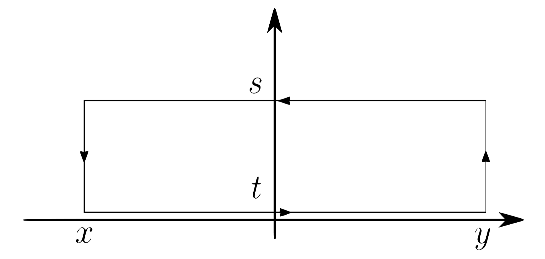
Because of its geometry, parallel transport along $\gamma_{R}$ can be readily expressed in terms of the monodromy matrices

$$\begin{aligned} \Omega_{\gamma_{R}}&=S(t,s,\lambda;x)T(y,x,\lambda;t)S(s,t,\lambda;y)T(x,y,\lambda;s)=\mathbb{1}\end{aligned}\;.$$

(31)

As a particular case, we get the following inversion property

$$\left\{\begin{aligned} &T(y,x,\lambda;\tau)=T^{-1}(x,y,\lambda;\tau)\\ &S(t,s,\lambda;z)=S^{-1}(s,t,\lambda;z)\end{aligned}\right.\;,$$

(32)

which in turn can be used to write Eq. (31) as

$$T(x,y,\lambda;t)=S(s,t,\lambda;y)\;T(x,y,\lambda;s)\;S^{-1}(s,t,\lambda;x)$$

(33)

This expression is particularly useful whenever the two points $x$ and $y$ are such that for all values of $\lambda$ and all times $\tau\in[s,t]$, one has:

$$V(x,\tau,\lambda)=V(y,\tau,\lambda)\;,$$

(34)

In such a case, $S(s,t,\lambda;x)=S(s,t,\lambda;y)$ and equation (33) implies that the time evolution of the monodromy matrix $T(x,y,\lambda)$ just amounts to a gauge transformation. In particular, we get that the trace of the monodromy matrix $\mathrm{Tr}\left[T(x,y,\lambda)\right]$ is constant in time for all $\lambda$

	$\displaystyle\mathrm{Tr}\left[T(x,y,\lambda;t)\right]$	$\displaystyle=\mathrm{Tr}\left[S(s,t,\lambda;y)\;T(x,y,\lambda;s)\;S^{-1}(s,t,\lambda;x)\right]$		(35)
		$\displaystyle=\mathrm{Tr}\left[T(x,y,\lambda;s)\right]\;$

In what follows, we will use this property to build a generating function for the constants of motion.

In order to compute all the conserved quantities one first needs to write the monodromy matrix as a Poincaré expansion in $\lambda$ Faddeev and Takhtajan 2007.

We first introduce the monodromy matrix $E(y-x,\lambda)$ associated with Eqs. (21) for the trivial constant solution $\Phi(x,t)=0$, $\Gamma(x,t)=0$

	$\displaystyle E(y-x,\lambda)$	$\displaystyle=\lim_{\Phi\to 0}\lim_{\Gamma\to 0}\left[\mathcal{P}\exp\int_{x}^{y}U(z,t,\lambda)dz\right]$		(36)
		$\displaystyle=\exp\left[\frac{\lambda}{2}(y-x)\sigma_{3}\right]\;,$

where

$$\sigma_{3}=\begin{pmatrix}1&0\\ 0&-1\end{pmatrix}\;.$$

(37)

The monodromy matrix can then be written as an expansion in inverse powers of $\lambda$

	$\displaystyle T(x,y,\lambda;t)$	$\displaystyle=E(y-x,\lambda)+\sum_{n=0}^{\infty}\frac{T_{n}(x,y;t)E(y-x,\lambda)}{\lambda^{n+1}}$		(38)
		$\displaystyle+\sum_{n=0}^{\infty}\frac{\tilde{T}_{n}(x,y;t)E(x-y,\lambda)}{\lambda^{n+1}}\;.$

To each order in this expansion we will show that there is an associated conserved quantity.

To achieve this we look for an expression for the monodromy matrix in the form

$$T(x,y,\lambda;t)=\left(\mathbb{1}+W(y,\lambda;t)\right)\exp Z(x,y,\lambda;t)\left(\mathbb{1}+W(x,\lambda;t)\right)^{-1}\;,$$

(39)

where $W$ and $Z$ are respectively an off-diagonal and a diagonal matrix, with the following Poincaré expansions Faddeev and Takhtajan 2007

$$W(y,\lambda;t)=\sum_{n=0}^{\infty}\frac{W_{n}(y;t)}{\lambda^{n+1}}\;,$$

(40)

and

$$Z(x,y,\lambda;t)=E(y-x,\lambda)+\sum_{n=0}^{\infty}\frac{Z_{n}(x,y;t)}{\lambda^{n+1}}\;.$$

(41)

Starting from the first order differential equation fulfilled by the monodromy matrix $T$:

$$\partial_{y}T(x,y,\lambda;t)=U(y,t,\lambda)T(x,y,\lambda;t)\;,$$

(42)

with initial condition

$$T(x,y,\lambda;t)|_{x=y}=\mathbb{1}\;,$$

(43)

we solve recursively this equation using the representation (39), proving in turn its validity.

Inserting the expression (39) in equation (42), and separating diagonal and off-diagonal parts, one obtains

$$\left\{\begin{aligned} &\partial_{y}Z(x,y,\lambda;t)=\frac{\lambda}{2}\sigma_{3}+U_{0}(y,t)W(y,\lambda;t)\\ &\partial_{y}W(y,\lambda;t)+W(y,\lambda;t)\partial_{y}Z(x,y\lambda;t)=U_{0}(y,t)+\frac{\lambda}{2}\sigma_{3}W(y,\lambda;t)\end{aligned}\right.\;,$$

(44)

where we have used the shorthand notation $U_{0}(x,y)\equiv U(y,t,0)$. Eliminating $Z(x,y,\lambda;t)$ between the two equations (44) on gets that $W(y,\lambda;t)$ is solution of a Riccati equation

$$\partial_{y}W-\lambda\sigma_{3}W+WU_{0}W-U_{0}=0\;.$$

(45)

Using expansion (40) one gets a solution of (45) as a recursion relation:

$$W_{n+1}=\sigma_{3}\left[\partial_{y}W_{n}+\sum_{k=0}^{n-1}W_{k}U_{0}W_{n-k}\right]\;,$$

(46)

with

$$W_{0}=-\sigma_{3}U_{0}\;.$$

(47)

More explicitly, if we write

$$W=\kappa_{\epsilon}\begin{pmatrix}0&\displaystyle{-\sum_{n=0}^{\infty}\frac{1}{\lambda^{n+1}}\,\tilde{w}_{n}}\\ \displaystyle{\sum_{n=0}^{\infty}\frac{1}{\lambda^{n+1}}\,w_{n}}&0\end{pmatrix}\;,$$

(48)

the recursion relation (46) becomes

$$\left\{\begin{aligned} &w_{n+1}=-\partial_{y}w_{n}+\epsilon\,\nu\,\Phi\sum_{k=0}^{n-1}w_{k}w_{n-k-1}\\ &\tilde{w}_{n+1}=\partial_{y}\tilde{w}_{n}+\epsilon\,\nu\,\Gamma\sum_{k=0}^{n-1}\tilde{w}_{k}\tilde{w}_{n-k-1}\\ \end{aligned}\right.\;,$$

(49)

with

$$\left\{\begin{aligned} &w_{0}=\Gamma\\ &\tilde{w}_{0}=\Phi\\ \end{aligned}\right.\;.$$

(50)

Now, the first equation in (44) can be readily integrated as

$$Z(x,y,\lambda;t)=\frac{\lambda(y-x)}{2}\,\sigma_{3}+\int_{x}^{y}U_{0}(z,t)W(z,\lambda;t)dz\;.$$

(51)

Using expansion (49) this last expression becomes

$$\begin{aligned} Z(x,y,\lambda;t)&=\frac{\lambda(y-x)}{2}\begin{pmatrix}1&0\\ 0&-1\end{pmatrix}\\ &+\kappa_{\epsilon}\,\begin{pmatrix}\displaystyle{\sum_{n=0}^{\infty}\frac{1}{\lambda^{n+1}}\int_{x}^{y}w_{n}\Phi dz}&0\\ 0&\displaystyle{-\sum_{n=0}^{\infty}\frac{1}{\lambda^{n+1}}\int_{x}^{y}\tilde{w}_{n}\Gamma dz}\end{pmatrix}\end{aligned}\;$$

(52)

By way of equations (49) and (50), it is easy to check that for all $n$

$$\int_{x}^{y}w_{n}(z,t)\Phi(z,t)dz=\int_{x}^{y}\tilde{w}_{n}(z,t)\Gamma(z,t)dz\;$$

(53)

Thus we have

$$Z(x,y,\lambda;t)=\left[\frac{1}{2}\lambda(y-x)+\kappa_{\epsilon}^{2}\,\sum_{n=0}^{\infty}\frac{1}{\lambda^{n+1}}\int_{x}^{y}w_{n}(z,t)\,\Phi(z,t)\,dz\right]\sigma_{3}$$

(54)

and we obtain from equation (39)

$$\begin{aligned} \mathrm{Tr}\left[T\right]&=\mathrm{Tr}\left[\exp Z\right]\\ &=2\mathrm{ch}\left[\lambda(y-x)-\epsilon\nu\sum_{n=0}^{\infty}\frac{1}{\lambda^{n+1}}\int_{x}^{y}w_{n}(z,t)\Phi(z,t)dz\right]\end{aligned}\;,$$

(55)

meaning that for all $n$ the integral (53) has to be constant in time. Integrals of motion are obtained by computing the monodromy matrix over the whole space, letting the interval $]x,y[\rightarrow\mathbb{R}$. In this limit, the first term inside the right hand side of Eq. (55) diverges but this can be dealt with using a standard renormalisation procedure (cf Appendix B). Up to a $\nu^{-1}$ factor due to rescaling of lengths (21), one finds the same conserved quantities obtained through (14). Indeed the first three quantities read

$$\begin{aligned} &Q_{0}=\int_{\mathbb{R}}w_{0}\Phi dx=\int_{\mathbb{R}}\Gamma\Phi dx\,=\,\frac{1}{\nu}\,N\\ &Q_{1}=\int_{\mathbb{R}}w_{1}\Phi dx=\frac{1}{2}\int_{\mathbb{R}}(\Gamma\partial_{x}\Phi-\Phi\partial_{x}\Gamma)dx\,=\,\,P\\ &Q_{2}=\int_{\mathbb{R}}w_{2}\Phi dx=\int_{\mathbb{R}}(-\partial_{x}\Phi\partial_{x}\Gamma+\epsilon\,\nu\,\Phi^{2}\,\Gamma^{2})dx\,=\,\frac{2}{|g|}\,E\end{aligned}\qquad,$$

(56)

and one can check that these are indeed equivalent to the conserved quantities $N$, $P$ and $E$ introduced in section II.2. Higher order terms correspond to more abstract quantities we will not discuss but are still, by construction, invariant.

For the MFG equations (2) to be completely integrable in the Liouville sense, the (infinite number of) conserved quantities generated in section IV.1 need to be in involution. Here, we introduce a Poisson structure in the context of integrable MFGs and use it to show the Poisson commutativity of the aforementioned conserved quantities. Here again this amounts to adapting a standard procedure Babelon et al. 2003, presented in the present context for the sake of completeness.

References

- Lasry and Lions (2006a) J.-M. Lasry and P.-L. Lions, Comptes Rendus Mathematique 343, 619 (2006a).
- Lasry and Lions (2006b) J.-M. Lasry and P.-L. Lions, Comptes Rendus Mathematique 343, 679 (2006b).
- Lasry and Lions (2007) J.-M. Lasry and P.-L. Lions, Japanese Journal of Mathematics 2, 229 (2007).
- Huang et al. (2006) M. Huang, R. P. Malhamé, P. E. Caines, and others, Communications in Information & Systems 6, 221 (2006).
- Lachapelle et al. (2009) A. Lachapelle, J. Salomon, and G. Turinici, Les Cahiers de la Chaire (Finance Développement Durable) 16 (2009).
- Cardaliaguet and Lehalle (2017) P. Cardaliaguet and C.-A. Lehalle, Math Finan Econ 12, 335 (2017).
- Carmona et al. (2013) R. Carmona, F. Delarue, and A. Lachapelle, Mathematics and Financial Economics 7, 131 (2013).
- Achdou et al. (2016) Y. Achdou, P.-N. Giraud, J.-M. Lasry, and P.-L. Lions, Appl. Math. Optim. 74, 579–618 (2016).
- Achdou et al. (2014) Y. Achdou, F. J. Buera, J.-M. Lasry, P.-L. Lions, and B. Moll, Phil. Trans. R. Soc. A 2014, 372, (2014).
- Guéant et al. (2011) O. Guéant, J.-M. Lasry, and P.-L. Lions, in Paris-Princeton Lectures on Mathematical Finance 2010 (Springer, 2011).
- Kizilkale and Malhame (2016) A. C. Kizilkale and R. P. Malhame, in Control of Complex Systems (Elsevier, 2016) pp. 559–584.
- Kizilkale et al. (2019) A. C. Kizilkale, R. Salhab, and R. P. Malhamé, Automatica 100, 312 (2019).
- Mériaux et al. (2012) F. Mériaux, V. Varma, and S. Lasaulce, in 2012 conference record of the forty sixth Asilomar conference on signals, systems and computers (ASILOMAR) (IEEE, 2012) pp. 671–675.
- Ullmo et al. (2019) D. Ullmo, I. Swiecicki, and T. Gobron, Physics Reports 799, 1 (2019).
- Bonnemain et al. (2020a) T. Bonnemain, D. Ullmo, and T. Gobron, to be published in SciPost Physics , arXiv:2006.01221 (2020a).
- Bonnemain et al. (2020b) T. Bonnemain, T. Gobron, and D. Ullmo, Physics Letters A 384, 126608 (2020b).
- Swiecicki (2016) I. Swiecicki, Étude de quelques modèles issus de la théorie des jeux en champs moyens. (PhD thesis, Université Cergy-Pontoise, 2016).
- Swiecicki et al. (2016) I. Swiecicki, T. Gobron, and D. Ullmo, Phys. Rev. Lett. 116, 128701 (2016).
- Liouville (1855) J. Liouville, Journal de Mathématiques pures et appliquées , 137 (1855).
- Arnol’d (2013) V. I. Arnol’d, Mathematical methods of classical mechanics, Vol. 60 (Springer Science & Business Media, 2013).
- Guéant (2012) O. Guéant, Math. Models Methods Appl. Sci. 22, 1250022 (2012).
- Shabat and Zakharov (1972) A. Shabat and V. Zakharov, Soviet physics JETP 34, 62 (1972).
- Novikov et al. (1984) S. Novikov, S. Manakov, L. Pitaevskii, and V. E. Zakharov, Theory of solitons: the inverse scattering method (Springer Science & Business Media, 1984).
- Faddeev and Takhtajan (2007) L. Faddeev and L. Takhtajan, Hamiltonian methods in the theory of solitons (Springer Science & Business Media, 2007).
- Ablowitz and Segur (1981) M. J. Ablowitz and H. Segur, Solitons and the inverse scattering transform (SIAM, 1981).
- Ambrose and Singer (1953) W. Ambrose and I. M. Singer, Trans. Amer. Math. Soc 75, 428 (1953).
- Babelon et al. (2003) O. Babelon, D. Bernard, M. Talon, C. U. Press, P. Landshoff, D. Nelson, D. Sciama, and S. Weinberg, Introduction to Classical Integrable Systems, Cambridge Monographs on Mathematical Physics (Cambridge University Press, 2003).
- (28) By analogy with finite-dimensional coordinates, x may be thought of a coordinate label.
- (29) This can naturally be generalized to matrices, but we restrict the discussion to matrices of the size of .
- Bonnemain (2020) T. Bonnemain, Quadratic Mean Field Games with Negative Coordination, Theses, Université Cergy Pontoise (2020).
- Ablowitz et al. (1974) M. J. Ablowitz, D. J. Kaup, A. C. Newell, and H. Segur, Studies in Applied Mathematics 53, 249 (1974).
- Avan and Caudrelier (2017) J. Avan and V. Caudrelier, Journal of Geometry and Physics 120, 106 (2017).
- Broda (2001) B. Broda, Advances in Chemical Physics 119, 429 (2001).