Equivalent Classification Mapping for Weakly Supervised Temporal Action Localization
Abstract
Weakly supervised temporal action localization is a newly emerging yet widely studied topic in recent years. The existing methods can be categorized into two localization-by-classification pipelines, i.e., the pre-classification pipeline and the post-classification pipeline. The pre-classification pipeline first performs classification on each video snippet and then aggregate the snippet-level classification scores to obtain the video-level classification score. In contrast, the post-classification pipeline aggregates the snippet-level features first and then predicts the video-level classification score based on the aggregated feature. Although the classifiers in these two pipelines are used in different ways, the role they play is exactly the same—to classify the given features to identify the corresponding action categories. To this end, an ideal classifier can make both pipelines work. This inspires us to simultaneously learn these two pipelines in a unified framework to obtain an effective classifier. Specifically, in the proposed learning framework, we implement two parallel network streams to model the two localization-by-classification pipelines simultaneously and make the two network streams share the same classifier. This achieves the novel Equivalent Classification Mapping (ECM) mechanism. Moreover, we discover that an ideal classifier may possess two characteristics: 1) The frame-level classification scores obtained from the pre-classification stream and the feature aggregation weights in the post-classification stream should be consistent; 2) The classification results of these two streams should be identical. Based on these two characteristics, we further introduce a weight-transition module and an equivalent training strategy into the proposed learning framework, which assists to thoroughly mine the equivalence mechanism. Comprehensive experiments are conducted on three benchmarks and ECM achieves accurate action localization results.
Index Terms:
Equivalent mechanism, temporal action localization, post-classification pipeline, pre-classification pipeline.I Introduction
Temporal action localization aims to localize action instances from the given untrimmed video by determining the start temporal points, end temporal points, and the corresponding action categories. In the studied weakly supervised setting, the action localizers are learned directly from video-level labels, without requiring fine segment-level annotations.

Consequently, weakly supervised temporal action localization can alleviate the burdensome and expensive human annotation. Moreover, it is potential to further realize the learning process on web-scale unlabeled videos and achieve breakthroughs.
In order to eliminate the ambiguity brought by the weak supervision, most previous works adopt the localization-by-classification pipelines to estimate the video-level classification score, which can be categorized into two main pipelines, i.e., the pre-classification pipeline (see Figure 1(a)) and the post-classification pipeline (see Figure 1(b)). Among the existing methods, UntrimmedNet [1] makes the pioneering exploration for the pre-classification pipeline. It first performs classification at each temporal point to obtain the class activation sequence, which is then aggregated to predict the video-level classification score. Based on this work, CMCS [2] proposes a diversity loss to model the completeness of actions. Meanwhile, 3C-Net [3] introduces action count cues to distinguish adjacent action sequences. In aforementioned pre-classification pipelines, the classification mapping functions are learned based on each temporal point and its corresponding local neighbors. Such a mechanism would be beneficial to capturing local contrast information but tends to be less effective in perceiving long-term connections within each given video.
Apart from pre-classification pipelines, there are also works, such as [4, 5, 6], which adopt the post-classification pipelines. These works first aggregate features from all temporal points to form the video-level feature representation, then they predict the video-level classification scores by classifying the aggregated feature representation. The advantage of these methods is that the aggregated feature can represent long-term relationships. However, when performing classification at each temporal point in the evaluation phase, the class activation sequences generated by these methods show insufficient discriminability to localize actions that belong to different categories.
From above discussions, we can observe that both the pre-classification pipeline and the post-classification pipeline aim at learning the effective classification mapping functions to predict the classification scores from the input features. The difference is that the pre-classification pipeline uses the classifier to perform classification on feature of each temporal point, while the post-classification pipeline uses the classifier to perform classification on the aggregated feature of the whole video sequence. Note that the post-classification pipeline uses weighted sum to aggregate snippet features. By such a linear operation, the aggregated feature remains in the same feature space with point-level features. When an ideal classification mapping function is given, both pipelines would obtain accurate classification results. This inspires us to simultaneously learn these two pipelines under a newly proposed Equivalent Classification Mapping (ECM) mechanism to obtain the desired classifier. After this, the learned classifier can be used to identify the presence of actions on each temporal point.
The framework of ECM is shown in Figure 2. Compiling the basic equivalent classification mapping spirit, ECM adopts two parallel network streams to model the pre-classification pipeline and the post-classification pipeline, respectively, and makes these two network streams share the same classifier. This simple and direct implementation of the equivalent classification mapping mechanism brings adequate performance gains over both the pre-classification baseline and the post-classification baseline. However, there are still non-negligible performance gaps when compared with state-of-the-art methods, indicating that adequately mining the equivalence mechanism is critical for good results.
We propose two equivalence-based components to thoroughly explore the equivalence mechanism: the module and the equivalent training strategy. The weight-transition module is designed to learn precise attention weights for the post-classification stream. Specifically, ECM transits the frame-level classification scores obtained from the pre-classification stream to generate the feature aggregation weights for the post-classification pipeline. This is different from traditional post-classification pipelines [4, 5, 6], where the feature aggregation weights are inferred in self-attention-like manners. Moreover, apart from the basic classification losses of each network stream, we introduce a novel equivalent training strategy, which contains a classification-to-classification consistency loss and an aggregation-to-classification consistency loss. The former is designed to penalize the inconsistency of the classification scores from two network streams, while the latter is designed to penalize the inconsistency of the classification score and the aggregation weights. In summary, the weight-transition module and the equivalent training strategy assist to adequately mine the equivalence mechanism between the pre-classification stream and the post-classification stream. This improves the performance of ECM and results in accurate action localization results.
The contribution of this work can be summarized as follows:
- •
ECM reveals the equivalence mechanism, indicating that both the classification for snippet features in the pre-classification pipeline and the classification for aggregated features in the post-classification pipeline pursue the same ideal classifier. Although conceptually simple, the equivalence mechanism is overlooked by previous methods, but plays an essential role in localizing actions under weak supervision.
- •
We propose two equivalence-based components, i.e., the weight-transition module and the equivalent training strategy, to adequately mine the equivalence mechanism. A simple and direct implementation of the equivalence mechanism shows improvements over baselines, which can be further promoted by these two equivalence-based components.
- •
Empirically, ECM starts from two simple and widely used baselines (with performance and ), employs equivalence-based components, explores the equivalence mechanism, and achieves accurate localization performance ( on THUMOS14) without bells and whistles. Considering its simplicity, ECM can serve as a solid baseline for future studies.
II Related Work
II-A Action recognition
Action recognition is a fundamental task for video analysis and understanding. With the development of deep learning, many effective algorithms have emerged. An early classic work is [7], which adopts a two-stream ConvNet architecture, to incorporate single frame RGB image and multi-frame optical flow. Then, C3D [8] uses 3D ConvNets for spatiotemporal feature learning. Next, I3D [9] proposes a new Two-Stream Inflated 3D ConvNet and P3D ResNet [10] fully exploits ResNet by simulating 3D CNN. Recently, Feichtenhofer et al. propose SlowFast [11] networks for video recognition. However, all these methods learn from trimmed videos, but real applications usually encounter untrimmed videos.

II-B Supervised action localization
Supervised action localization task learns from precisely annotated action instances and can deal with untrimmed videos which contain a large percentage of backgrounds. Early explorations adopt a detection-by-classification pipeline. S-CNN [12] classifies sliding-window proposals to localize action instances. CDC [13] and Lin et al. [14] predict the actionness score for each temporal point. Meanwhile, advances in object detection bring inspiration to action localization. Some methods follow Faster R-CNN [15] and perform two-stage action localization, e.g., R-C3D [16] and TAL [17]. Similarly, some methods follow one-stage object detection methods [18] and perform action localization, e.g., SSAD [19] and GTAN [20]. In addition, the recurrent memory module is used to capture long-term dependencies, such as SS-TAD [21], SST [22]. Apart from the above explorations, some noticeable works also include modeling temporal structure [23], modeling context [17, 24], modeling relationships among action proposals [25], localizing action instances from a part of videos [26], etc. Recently, Yang et al. propose A2Net [27] which adopts a novel anchor-free action localization module to tackle extremely short action instances or extremely long ones. G-TAD [28] presents a graph convolutional network model to exploit video context and cast temporal action localization as a sub-graph detection problem. Zhao et al. [29] introduce two regularization terms to alleviate the problem of incorrect or inconsistent predictions. In summary, supervised methods can explicitly learn from segment-level annotations and achieve accurate localizations. However, they are limited by the expensive annotations as well, which can be alleviated by the studied weakly supervised method.
II-C Weakly supervised action localization
Weakly supervised action localization task only requires video-level category information in the training phase. The previous methods can be divided into two categories, i.e., the pre-classification pipeline and the post-classification pipeline. In the pre-classification pipeline, UntrimmedNets [1] performs classification at each video snippet, then aggregates snippet scores at temporal dimension to obtain video-level classification scores. Later, W-TALC [30] considers the co-activity similarity to model inter-video similarities and differences. Furthermore, CMCS [2] proposes to jointly learn multiple classification networks and require them to generate diverse responses. Focused on the quality of the class activation sequence, there are some other promising works. CleanNet [31] learns regression to adjust the action segments. TSM [32] models the action structure via a multi-phase process. 3C-Net [3] introduces multi-label center loss to obtain discriminative feature representation. BaSNet [33] tries to suppress the background response by giving different background labels on two branches. Recently, Gong et al. [34] propose to learn class-specific and class-agnostic attention simultaneously. A2CL-PT [35] adopts an adversarial approach to obtain more complete action instances. TSCN [36] presents two-stream consensus network to eliminate false positive action proposals and improve localization boundaries. EM-MIL [37] explicitly models latent variables and adopts an expectation-maximization framework to better model the background information. In general, the foundation of pre-classification methods is the class activation sequence, generated by the classification mapping function.
Apart from the above methods, there is another pipeline, namely the post-classification pipeline. Inspired by the success of CAM [38], STPN [4] proposes to first aggregate video features then perform classification. Later, Nguyen et al. [5] extend STPN [4] by introducing background modeling and top-down class-guided attention. Meanwhile, MAAN [6] develops the post-classification pipeline with a marginalized average aggregation module. Recently, Shi et al. [39] use conditional variational auto-encoder to model the frame-wise representation conditioned for tackling action-context confusion issue. In general, the post-classification pipeline is aware of the complete video features, but its response to each temporal point may be not discriminative enough.
III Method

Given a dataset containing action categories, each video in the dataset has the classification label , where indicates whether there is an action instance belonging to category . Each video is firstly divided into snippets and then a feature extractor is used to extract the feature representation from each video snippet. Under the weakly supervised learning scenario, ECM learns the classifier from the video-level classification label , is the specific sub-classifier for category , aiming at discovering the temporal locations of the desired action instances for each video.
III-A The body network
As shown in Figure 2, the body network consists of two streams: the pre-classification stream and the post-classification stream. They share the same classification mapping function but make predictions in different manners.
We start the elaboration of ECM from a concise mathematical proof that the point-level features in the pre-classification branch and aggregated video-level features in the post-classification branch lie in the same feature space, and they require an identical ideal classifier. Suppose the ideal classifier for pre-classification stream and post-classification stream is and , respectively. Given snippet features , we adopt weighted sum operation to aggregate features and obtain , i.e., , where is the weight for . Because weighted sum is a linear operation, is in the same feature space with . Moreover, as for feature space , there exists one optimal classifier that can precisely classify most number of features. Because , the two streams aim to learn an identical ideal classifier.
To endow the classifier with the helpful temporal reception field, we use three temporal convolutional layers to build it (see Figure 2), where the kernel sizes of the first two layers are while it of the last layer is . Here, the classifier is used to predict the classification scores for each temporal point, i.e., each video snippet. Specifically, in the pre-classification stream, original video features are directly passed through the classifier. Then, the network obtains classification scores along temporal points and generates class activation sequences for the whole video. After that, we adopt the top- mean strategy to aggregate the classification scores for each category and obtain the video-level classification score .
In the post-classification stream, the inputs consist of both the video features and the category-specific aggregation weights. Here, we explore both action weights and background weights to generate the category-specific action features and category-specific background features , where .
In detail, the category-specific feature for either action or background is obtained by weighted sum operation over the video features :
| (1) |
| (2) |
where and are elements in and , respectively. Then, each sub-classifier is applied to the corresponding category-specific action feature to obtain the final classification score , where , denotes the network forward operation.
The classifier is shared between the pre-classification stream and the post-classification stream, where the first layer adopts temporal convolution with kernel size . Consequently, the post-classification stream requires the temporal length of the aggregated feature to be . Given video features and class-specific aggregation weights, a direct weighted sum would generate one aggregated feature. In order to aggregate features for each category, we propose a specific feature aggregation strategy, as shown in Figure 3. First of all, we evenly divide video features as well as the corresponding aggregation weights into three folds by sampling every three snippets. Then, we perform feature aggregation and generate features for each category. After that, feature vectors belonging to the same category are re-organized together. Finally, category-specific features are sent to the corresponding sub-classifier to predict video-level classification scores. Comparing to the strategy that directly extracting the whole video features in one fold, the aggregated video-level features extracted by our strategy can better fit the input structure of the classifier, thus facilitating a more effective equivalent learning scheme.

III-B Equivalent weight-transition module
The post-classification stream requires category-specific aggregation weights and to aggregate features. Considering that the class activation sequence obtained from the pre-classification stream can reveal the probability that a temporal point belongs to an action instance, we propose to obtain the aggregation weights by transiting the class activation sequence, as shown in Figure 4. We use a convolutional layer with kernel size to predict the importance values for each temporal point. After that, we apply the sigmoid activation and obtain the action aggregation weights , while the background aggregation weights can be obtained via . Compared with the conventional methods [4, 5, 6, 33], the proposed equivalent weight-transition module shows two characteristics. Firstly, existing works adopt an extra network to predict the aggregation weights, while the proposed module can directly obtain aggregation weights from the pre-classification stream. Besides, existing methods predict category-agnostic weights and use them to obtain one aggregated feature to represent the input video. In contrast, we learn category-specific weights and use them to obtain aggregated features for each different action categories. Such category-specific features would bring richer representation and assist ECM to clearly distinguish different action categories, as verified in Section IV-C.
III-C Classification-to-classification consistency
The equivalent training strategy consists of a classification-to-classification consistency loss and an aggregation-to-classification consistency loss . Given an input video, the pre-classification stream predicts the classification score , while the post-classification stream predicts the classification score with action aggregation weights . Based on the intuition that the classification scores predicted by the two network streams should be identical for the same input video, we introduce the classification-to-classification consistency loss to the learning process:
| (3) |
The classification-to-classification consistency term plays a role in making one stream perceive the predictions from the other stream. Despite the simplicity, it obviously facilitates the learning of the classification mapping function, as shown in Section IV-C.
III-D Aggregation-to-classification consistency
Besides classification-to-classification consistency, we further explore the aggregation-to-classification consistency loss. The motivation is that the video-level classification score should be consistent with the aggregation weights. Specifically, the proposed aggregation-to-classification loss not only requires the action attention weights to highlight snippets within an action, but also requires the background attentions to exclude all action snippets. It assists the learning of the attention weights with considerations about both action presence and action absence. This training strategy is different from conventional classification loss, where the attention weights may only highlight the most discriminative snippets within an action but still can correctly predict video-level classification label.
Considering a video with classification label , the post-classification stream can predict the action presence score with action weights . Meanwhile, it can predict the action absence score with background weights . Similar to the action presence score , the action absence score is obtained by . Then, for an input video that contains action categories, we select classification scores for presenting action categories from and according to classification label . After that, we define , which corresponds to positive labels and negative labels. Finally, the aggregation-to-classification consistency loss can be calculated as follows:
| (4) |
The proposed aggregation-to-classification consistency training strategy can guide ECM to better distinguish action segments and backgrounds. Besides, the existing background modeling strategy [5] and background suppression strategy [33] can be regarded as the specific cases of this strategy, where they only consider the background category when adjusting attention weights.
III-E Training and inference
| Sup. | Method | Pub. | feature | 0.50 | 0.55 | 0.60 | 0.65 | 0.70 | 0.75 | 0.80 | 0.85 | 0.90 | 0.95 | avg (0.50:0.95) | |
| Full | SSN [23] | ICCV 17 | TS | 41.3 | - | - | - | - | 27.0 | - | - | - | 6.1 | 26.6 | |
| Weak | Pre-Cls | AutoLoc [40] | ECCV 18 | UNT | 27.3 | 24.9 | 22.5 | 19.9 | 17.5 | 15.1 | 13.0 | 10.0 | 6.8 | 3.3 | 16.0 |
| TSM [32] | ICCV 19 | I3D | 28.3 | 26.0 | 23.6 | 21.2 | 18.9 | 17.0 | 14.0 | 11.1 | 7.5 | 3.5 | 17.1 | ||
| W-TALC [30] | ECCV 18 | I3D | 37.0 | - | - | - | 14.6 | - | - | - | - | - | 18.0 | ||
| EM-MIL [37] | ECCV 20 | I3D | 37.4 | - | - | - | 23.1 | - | - | - | 2.0 | - | 20.3 | ||
| CleanNet [31] | ICCV 19 | I3D | 37.1 | 33.4 | 29.9 | 26.7 | 23.4 | 20.3 | 17.2 | 13.9 | 9.2 | 5.0 | 21.6 | ||
| 3C-Net [3] | ICCV 19 | I3D | 37.2 | - | - | - | 23.7 | - | - | - | 9.2 | - | 21.7 | ||
| CMCS [2] | CVPR 19 | I3D | 36.8 | - | - | - | - | 22.0 | - | - | - | 5.6 | 22.4 | ||
| BaSNet [33] | AAAI 20 | I3D | 38.5 | - | - | - | - | 24.2 | - | - | - | 5.6 | 24.3 | ||
| ACL [34] | CVPR 20 | I3D | 40.0 | - | - | - | - | 25.0 | - | - | - | 4.6 | 24.6 | ||
| Post-Cls | DGAM [39] | CVPR 20 | I3D | 41.0 | 37.5 | 33.5 | 30.1 | 26.9 | 23.5 | 19.8 | 15.5 | 10.8 | 5.3 | 22.4 | |
| TSCN [36] | ECCV 20 | I3D | 37.6 | - | - | - | - | 23.7 | - | - | - | 5.7 | 23.6 | ||
| Equ. | ECM | I3D | 41.0 | 37.7 | 34.2 | 31.5 | 28.5 | 24.9 | 21.2 | 17.0 | 12.1 | 6.5 | 25.5 | ||
In training, we calculate the classification loss and for the pre-classification stream and the post-classification stream, respectively. Formally, the classification problem can be formulated as a multi-label classification problem. We perform normalization on the original classification label and calculate the cross-entropy loss. Besides, the classification-to-classification consistency loss and the aggregation-to-classification consistency loss are also calculated to guide the mining of the equivalence mechanism. Thus, the complete loss function can be calculated as:
| (5) |
where and are trade-off coefficients to balance the effect of different losses.
When the training process is complete, we forward each input video through the learned classifier and obtain the class activation sequences. Then, following BaSNet [33], we discard categories whose classification scores are smaller than a threshold . After that, the remaining class activation sequences are min-max normalized along the temporal dimension, which is followed by the temporal actionness grouping operation [23] to localize action instances. Finally, redundant action instances are filtered out via NMS.
IV Experiments
IV-A Experimental setups
Dataset. We perform experiments on three benchmarks: THUMOS14 [41], ActivityNet v1.2 [42] and ActivityNet v1.3 [42]. THUMOS14 consists of action categories, including videos for training and videos for testing. ActivityNet v1.2 consists of action categories, videos. The video number ratio among training, validation and testing sets is ::. ActivityNet v1.3 is an extension of ActivityNet v1.2, with categories and videos.
Metric. The evaluation is performed under the official metric of each dataset, i.e., mean Average Precision (mAP). THUMOS14 focuses on mAP under threshold , while ActivityNet focuses on the average mAP under thresholds [::]. Following previous works [4, 5, 33], we adopt official evaluation tools of the ActivityNet dataset to perform evaluations.
Feature extraction. To extract features, each video is evenly divided into snippets and we uniformly sample frames from each snippet, similar to previous works [4, 5]. The optical flow is calculated via the TV-L1 [43] algorithm. I3D model [9] pre-trained on the Kinetics-400 dataset is used to extract video features, without finetuning on THUMOS14 [41] or ActivityNet v1.3 [42]. We extract both the appearance features and the motion features, which are concatenated together to represent the video sequence. The concatenated feature dimension is . Finally, the snippet number for THUMOS14, ActivityNet v1.2 and ActivityNet v1.3 are , and , respectively.
Training and evaluation details. ECM is implemented using PyTorch [44]. Adam [45] solver is used to optimize the network. For all experiments, we set batch size to , the learning rate to and the weight decay to . We train ECM with epochs, epochs and epochs for THUMOS14, ActivityNet v1.2 and ActivityNet v1.3, respectively. The parameters are empirically determined via gird search. Specifically, we set for the top- mean aggregation. The balance coefficients are and . In evaluation, the threshold to reject absent categories is .
IV-B Comparison with state-of-the-arts
Experiments on ActivityNet v1.2. Table I reports the performance on ActivityNet v1.2 dataset. Most methods adopt the I3D feature, while there are also UntrimmedNet features (UNT) [1]. The weakly supervised WTAL is developed by both the pre-classification pipeline and the post-classification pipeline. AutoLoc [40] firstly builds the foundation performance of . At the same time, W-TALC [30] achieves via exploring co-activity relationship. Later, CleanNet [31] proposes to learn regression. 3C-Net [3] strives to lean discriminative features via constraining centerness and action counts. CMCS [2] simultaneously learns multiple complementary class activation sequences. These above methods gradually improve the performance to [2].
| Sup. | Method | Pub. | Fea. | 0.5 | 0.75 | 0.95 | 0.50:0.95 | |
| Full | TCN [24] | ICCV 17 | TS | 36.4 | 21.2 | 3.9 | - | |
| TAL [17] | CVPR 18 | I3D | 38.2 | 18.3 | 1.3 | 20.2 | ||
| CDC [13] | CVPR 17 | - | 45.3 | 26.0 | 0.2 | 23.8 | ||
| TSA-Net [29] | ECCV 20 | I3D | 43.5 | 33.9 | 9.2 | 30.1 | ||
| PGCN [25] | ICCV 19 | I3D | 48.3 | 33.2 | 3.3 | 31.1 | ||
| BMN [14] | ICCV 19 | TS | 50.1 | 34.8 | 8.3 | 33.9 | ||
| G-TAD [28] | CVPR 20 | I3D | 50.4 | 34.6 | 9.0 | 34.1 | ||
| GTAN [20] | CVPR 19 | P3D | 52.6 | 34.1 | 8.9 | 34.3 | ||
| Weak | pre | TSM [32] | ICCV 19 | I3D | 30.0 | 19.0 | 4.5 | - |
| CMCS [2] | CVPR 19 | I3D | 34.0 | 20.9 | 5.7 | 21.2 | ||
| BaSNet [33] | AAAI 20 | I3D | 34.5 | 22.5 | 4.9 | 22.2 | ||
| ACL [34] | ECCV 20 | I3D | 36.8 | 22.0 | 5.2 | 22.5 | ||
| post | STPN [4] | CVPR 18 | I3D | 29.3 | 16.9 | 2.6 | - | |
| LTSR [46] | AAAI 19 | Res | 33.1 | 18.7 | 3.3 | 21.8 | ||
| MAAN [6] | ICLR 19 | I3D | 33.7 | 21.9 | 5.5 | - | ||
| TSCN [36] | ECCV 20 | I3D | 35.3 | 21.4 | 5.3 | 21.7 | ||
| WSBM [5] | ICCV 19 | I3D | 36.4 | 19.2 | 2.9 | - | ||
| ECM | I3D | 36.7 | 23.6 | 5.9 | 23.5 | |||
Recently, BaSNet [33] proposes to suppress the response of backgrounds. They simultaneously learns two streams, i.e., the base stream and the suppression stream, which share network weights but dispose of different input data and pursue different classification target for the background category. Although BaSNet [33] maintains two streams and share weights between them, both two streams essentially adopt the pre-classification pipeline. Experimentally, there are performance gaps between BaSNet [33] and ECM. This demonstrates the equivalence mechanism is more applicable than the individual pre-classification mechanism for learning a powerful classifier. Beyond, ACL [34] achieves and shows high performance. Based on the pre-classification pipeline, ACL [34] aggregates features from all temporal points, constructs triplet features and calculates cluster-based loss, so as to enhance discriminability. However, ACL [34] only relies on the pre-classification pipeline to learn the classifier and ignores the post-classification pipeline. In contrast, ECM not only aggregates features to form a global representation, but also reveals the equivalence mechanism. Learning the same classifier from both pre-classification pipeline and post-classification pipeline, ECM exceeds ACL [34] and builds new state-of-the-art performance.
Apart from pre-classification pipeline, DGAM [39] and TSCN [36] are two recently developed post-classification methods. DGAM [39] starts from WSBM [5] and optimizes attention weights via alternatively learning the generative attention module and the discriminative attention module. TSCN [36] adopts the pseudo ground truth to guide the learning of the attention weights and perform iterative refinement. Nevertheless, both DGAM [39] and TSCN [36] only explore the post-classification pipeline to learn the classifier. In contrast, ECM demonstrates obvious superiority by exploring the equivalence mechanism between the pre-classification pipeline and the post-classification pipeline.
In addition to weakly supervised methods, ActivityNet is also explored by fully supervised method, e.g., structured segment network [23]. SSN [23] proposes a pyramid network to model temporal structures of action instances. It is encouraging that ECM only mines video-level classification labels but achieves competitive performance with SSN [23]. This further demonstrates the efficiency of the proposed equivalence classification mapping mechanism.
Experiments on ActivityNet v1.3. The comparison experiments on ActivityNet v1.3 dataset is shown in Table II. Temporal action localization on ActivityNet v1.3 is thoroughly studied in recent years, where there are multiple fully supervised and weakly supervised methods. Pioneering fully supervised methods [24, 13] adopt the detection-by-classification strategy and achieve average mAP [13]. Later, two-stage methods [17, 29, 14] improve the performance to step-by-step. Besides, GTAN [20] is a representative one-stage method with high performance of . Recently, the graph-convolution method [25, 28] exhibits superiority on temporal action localization, and achieves the performance of [28].
As for weakly supervised methods, for one thing, BaSNet [33] and ACL [34] are representative pre-classification methods, achieving the performance of and , respectively. For another thing, STPN [4] makes an early exploration and proposes the post-classification pipeline. This is further developed by subsequent works, e.g., LTSR [46] achieves the performance of and TSCN [36] achieves the performance of .
In contrast to existing weakly supervised methods, ECM achieves average mAP and exhibits obvious performance gains over existing strong competitors. In detail, ECM reaches the performance of and under threshold and , respectively, showing high performance. Compared with fully supervised methods, on the one hand, ECM only learns from video-level classification labels but exceeds TCN [24] and TAL [17] which learn from instance-level annotations. On the other hand, there is obvious performance gap between ECM and state-of-the-art supervised methods (e.g., G-TAD [28], GTAN [20]), indicating the weakly supervised algorithm should be continuously developed.
| Sup. | Method | Pub. | Fea. | 0.1 | 0.2 | 0.3 | 0.4 | 0.5 | 0.6 | 0.7 | |
| Full | One Stage | CDC [13] | CVPR 17 | - | - | - | 40.1 | 29.4 | 23.3 | 13.1 | 7.9 |
| GTAN [20] | CVPR 19 | P3D | 69.1 | 63.7 | 57.8 | 47.2 | 38.8 | - | - | ||
| Two Stage | R-C3D [16] | ICCV 17 | - | 54.5 | 51.5 | 44.8 | 35.6 | 28.9 | - | - | |
| TSA-Net [29] | ECCV 20 | I3D | - | - | 53.9 | 50.7 | 45.4 | 38.0 | 28.5 | ||
| TAL [17] | CVPR 18 | I3D | 59.8 | 57.1 | 53.2 | 48.5 | 42.8 | 33.8 | 20.8 | ||
| Graph Based | G-TAD [28] | CVPR 20 | TS | - | - | 54.5 | 47.6 | 40.2 | 30.8 | 23.4 | |
| PGCN [25] | ICCV 19 | I3D | 69.5 | 67.8 | 63.6 | 57.8 | 49.1 | - | - | ||
| Weak | Pre-Classification | UntrimmedNet [1] | CVPR 17 | UNT | 44.4 | 37.7 | 28.2 | 21.1 | 13.7 | - | - |
| AutoLoc [40] | ECCV 18 | UNT | - | - | 35.8 | 29.0 | 21.2 | 13.4 | 5.8 | ||
| W-TALC [30] | ECCV 18 | I3D | 55.2 | 49.6 | 40.1 | 31.1 | 22.8 | - | - | ||
| CMCS [2] | CVPR 19 | I3D | 57.4 | 50.8 | 41.2 | 32.1 | 23.1 | 15.0 | 7.0 | ||
| CleanNet [31] | ICCV 19 | I3D | - | - | 37.0 | 30.9 | 23.9 | 13.9 | 7.1 | ||
| TSM [32] | ICCV 19 | I3D | - | - | 39.5 | 31.9 | 24.5 | 13.8 | 7.1 | ||
| BaSNet [33] | AAAI 19 | I3D | 58.2 | 52.3 | 44.6 | 36.0 | 27.0 | 18.6 | 10.4 | ||
| Post-Classification | STPN [4] | CVPR 18 | I3D | 52.0 | 44.7 | 35.5 | 25.8 | 16.9 | 9.9 | 4.3 | |
| MAAN [6] | ICLR 19 | I3D | 59.8 | 50.8 | 41.1 | 30.6 | 20.3 | 12.0 | 6.9 | ||
| WSBM [5] | ICCV 19 | I3D | 64.2 | 59.5 | 49.1 | 38.4 | 27.5 | 17.3 | 8.6 | ||
| TSCN [36] | ECCV 20 | I3D | 63.4 | 57.6 | 47.8 | 37.7 | 28.7 | 19.4 | 10.2 | ||
| DGAM [39] | CVPR 20 | I3D | 60.0 | 54.2 | 46.8 | 38.2 | 28.8 | 19.8 | 11.4 | ||
| Equivalent | ECM | I3D | 62.6 | 55.1 | 46.5 | 38.2 | 29.1 | 19.5 | 10.9 | ||
Experiments on THUMOS14. In Table III, we compare ECM with recent state-of-the-art temporal action localization methods, including both the weakly supervised methods and the supervised ones on THUMOS14 dataset.
The weakly supervised methods consist of pre-classification methods and post-classification methods, both of which are widely explored. The first baseline of pre-classification methods is built by UntrimmedNet [1]. It learns video recognition model from video-level classification labels of untrimmed videos, which additionally discovers action instances via thresholding class activation sequences and achieves mAP@=. After this, AutoLoc [40] proposes the outer-inner-contrastive loss to precisely determine boundaries for actions and reaches . The outer-inner-contrastive strategy is widely used for the evaluation process in subsequent works. Because the class activation sequence may only discover the most discriminative action parts, subsequent works aim at improving the quality of class activation sequences, via mining co-activity loss [30], learning multiple complementary class activation sequences CMCS [2], mining temporal structure [32]. Recently, BaSNet [33] achieves precise localization performance, i.e., mAP@=. Although above methods are able to improve the quality of class activation sequence to some extent, they essentially follow the pre-classification pipeline. Specifically, only local features of each point are used to learn the classifier, while lacking consideration to the global video features. As a result, ECM exceeds these methods with at least performance gains, under the guidance of the equivalence mechanism. Apart from above methods, we note that some recent methods [34, 35, 37, 47] achieve high performance on THUMOS14 dataset. It should be noticed that these methods are somewhat complicated. For example, ActionBytes [47] is designed to generate action proposals, which are then combined with W-TALC [30] to localize action instances. EM-MIL [37] requires UntrimmedNet [1] or W-TALC [30] to classify action proposals. In contrast, ECM adopts a unified framework and a simple method, but achieves competitive performance. This demonstrates the efficiency of the equivalence classification mapping mechanism.
As for post-classification methods, STPN [4] is an early and extensively used baseline with performance mAP@=. Because attention weights have essential influence on aggregated video-level features, learning accurate attention weights becomes a research focus for subsequent works [6, 5, 36, 39]. Specifically, MAAN [6] proposes marginalized average aggregation, and WSBM [5] optimizes background attention weights. Recently, TSCN [36] and DGAM [39] build similar high performance under the metric mAP@, reaching and , respectively.
Compared with existing pre-classification methods and post-classification methods, ECM delves into both local features at each point and global features for the complete video to learn the classification network. Under the metric mAP@, ECM starts from simple pre-classification and post-classification baselines, and shows performance improvements over BaSNet [33], performance improvement over the strong competitor DGAM [39], without bells and whistles. This demonstrates the efficiency and superiority of the revealing equivalence mechanism.
Compared with fully supervised methods, on the one hand, ECM already exceeds some early methods, e.g., the one-stage method CDC [13] and the two-stage method R-C3D [16]. This demonstrates the efficiency of ECM for discovering action instances. On the other hand, the latest fully supervised methods achieve precise localization performance, e.g., PGCN [25] achieves under metric mAP@. This reminds us that the weakly supervised methods require further studies.
| Pre-Cls | ✓ | ✓ | ✓ | ☑ | ✓ | |
|---|---|---|---|---|---|---|
| Post-Cls | ✓ | ✓ | ✓ | ☑ | ✓ | |
| ✓ | ✓ | ✓ | ||||
| ✓ | ✓ | |||||
| mAP | 19.6 | 17.1 | 22.8 | 24.2 | 23.4 | 29.1 |
IV-C Ablation studies
Ablation studies about the equivalence mechanism. We perform ablation studies on the THUMOS14 dataset and report the results in Table IV. Under threshold , the pre-classification stream and the post-classification stream can achieve and , respectively. On this basis, we share the classifier between the pre-classification stream and the post-classification stream, transit the aggregation weights from the class activation sequence in the pre-classification stream. This direct and simple implementation of the equivalence mechanism reaches the performance of . Based on this, the proposed aggregation-to-classification consistency training strategy can lift the performance to . This supports our claim that constraining the consistency between aggregation weights and action presences. The aggregation-to-classification loss guides the classifier to perceive both action presence and action absence, so as to precisely localize the starting time and ending time of action instances. Moreover, the complete ECM achieves , under the cooperation of sharing the classifier, aggregation-to-classification loss and classification-to-classification loss . Furthermore, to clearly verify the efficiency of the equivalence classification mapping mechanism, we remove classifier sharing from ECM and keep all other components unchanged. Under this setting, the variant model obtains , which shows points inferior to the performance of ECM. This experiment demonstrates that classifier sharing (i.e., the equivalence mechanism) is the foundation of ECM, which effectively empowers the proposed equivalence-based components, i.e., the weight-transaction module, and the equivalent training strategy ( and ). Beyond this, we verify the effectiveness of class-specific feature representation. We follow existing methods [4, 5, 6] and learn class-agnostic aggregation weights for the post-classification stream, such a variant achieves the performance of . In contrast, the performance improvements of ECM owes to rich feature representations from the class-specific attention weights.
Differences with model ensemble. In implementation, ECM maintains two streams with weight sharing, which practice the equivalence classification mapping mechanism. ECM is essentially different from model ensemble methods. Specifically, ensemble methods usually train multiple models in parallel, generate multiple heterogeneous results, and fuse results to get improvements. In contrast, ECM learns one classifier from a unified learning framework (with a
| TH | Pre-Cls | Post-Cls | Merge | Weighted sum | |||
|---|---|---|---|---|---|---|---|
| 0.2 | 0.4 | 0.6 | 0.8 | ||||
| 0.1 | 46.1 | 42.3 | 45.5 | 43.5 | 44.2 | 44.9 | 45.1 |
| 0.2 | 38.8 | 35.8 | 39.2 | 36.6 | 37.4 | 38.2 | 38.4 |
| 0.3 | 32.1 | 29.1 | 33.0 | 30.7 | 31.2 | 31.9 | 32.1 |
| 0.4 | 25.3 | 23.1 | 26.5 | 24.9 | 25.5 | 26.0 | 26.3 |
| 0.5 | 19.6 | 17.1 | 21.4 | 20.2 | 20.3 | 20.5 | 20.8 |
| 0.6 | 12.7 | 11.0 | 13.8 | 13.4 | 13.9 | 14.3 | 14.4 |
| 0.7 | 7.2 | 6.2 | 7.9 | 8.2 | 8.2 | 8.3 | 8.4 |

two-stream architecture). In inference, ECM uses one model to predict one result rather than fusing results that are predicted by multiple models. Empirically, we perform ablation studies and report the results in Table V. If we independently train the pre-classification network and the post-classification network, the performance is and , respectively. There are two kinds of strategies to perform ensemble. The first one is action instances from two class activation sequences and merge the localization results. This strategy achieves under the metric mAP@. The
| Pre-Classification | Post-Classification | ECM | |
| Frame Accuracy | 42.7% | 39.0% | 54.3% |
second strategy is to fuse two class activation sequences and localize action instances from the fused sequence. Specifically, for class activation sequences from the pre-classification stream and the post-classification stream, we apply weight and , respectively. We carry out experiments with different , i.e., , , , and report the performance. The best performance is when . In general, the highest performance that model ensemble strategy can achieve is . In Table IV, a direct and simple implementation of the equivalence mechanism achieves , and the proposed equivalence-based components (i.e., the weight-transaction module and equivalent training strategy) can further mine the equivalence classification mapping mechanism and improve the performance to . The performance gap between model ensemble and ECM demonstrates the efficiency of the proposed equivalence mechanism, as well as the significant differences between ECM and model ensemble.
Frame Accuracy. In inference, the pre-classification method, the post-classification method and the proposed ECM method, all directly learn classifiers to predict the classification score for each temporal point. Following the frame accuracy metric adopted by the action segment researches [48], we measure the frame accuracy of the generated class activation sequences to validate the quality of the point-level classification. Similar to previous works [48], we do not consider the background points in order to prevent the case that a method predicts all frames as background but still achieves high performance.
Given the obtained class activation sequences, we first predict the video-level classification scores and reject categories whose classification scores are lower than threshold . Then, for the remaining responses, we perform max pooling and obtain the point-wise classification predictions. Finally, the frame-wise classification accuracy is reported in Table VI. It can be found that the pre-classification method performs somewhat better than the post-classification method, with a margin of . The proposed ECM brings obvious improvements, with a margin of . The results demonstrate that the proposed equivalent classification mapping mechanism can learn a high-quality classifier and can accurately discover action snippets in the untrimmed videos.
IV-D Qualitative Results
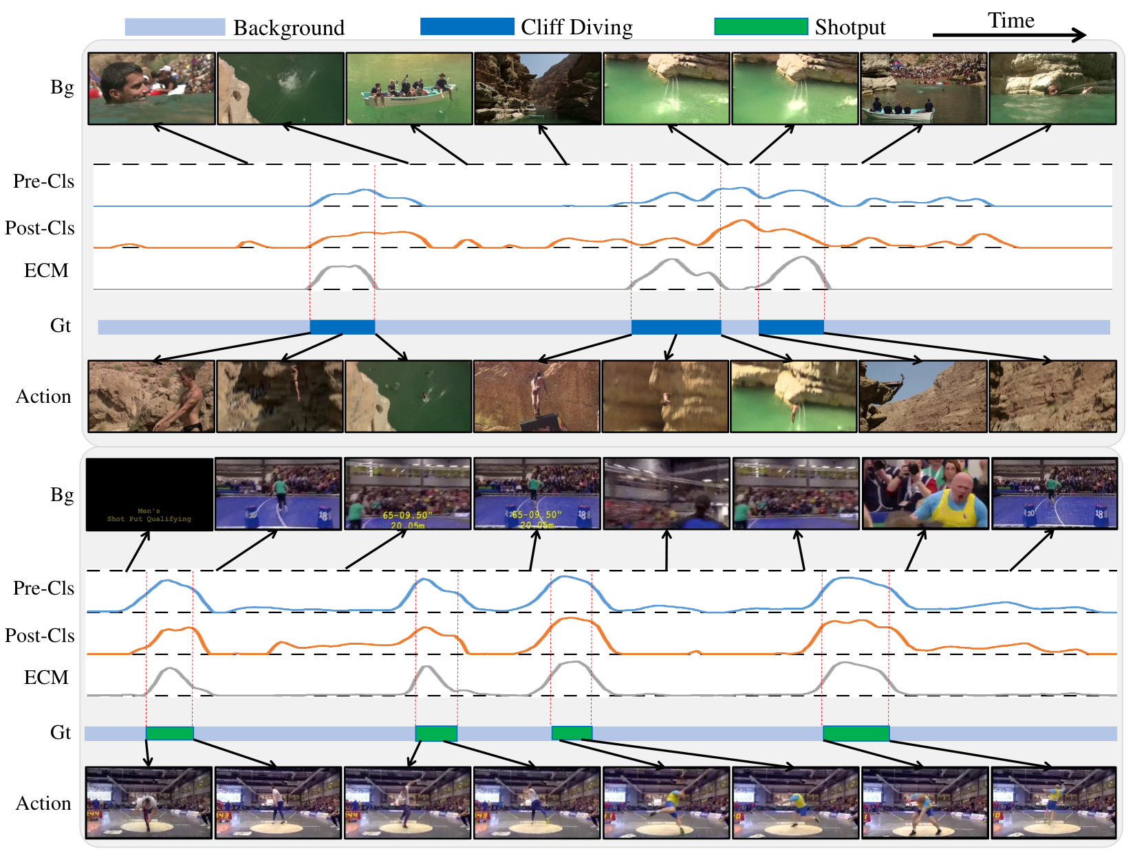
Visualization of action localizations. We qualitatively visualize the class activation sequences in Figure 5. When only using the pre-classification stream or the post-classification stream, the generated class activation sequences cannot distinguish two adjacent action instances (see the first case), or shows high responses for a part of background points (see the second case). This may lead to confusing localization results. In contrast, the proposed ECM method precisely shows high responses for action instances and confidently suppresses the response of backgrounds, leading to accurate localization results.
Visualization of feature distribution. At the beginning of Section III-A, it is proven that the aggregated video-level features lie in the same feature space with point-level features. In Figure 6, we use t-SNE [49] to visualize the feature distribution for point features and aggregated features. It is clear that action features and background features lie in different mainfolds. Besides, the aggregated video-level features lie in the same mainfold with the action features. This visualization supports our claim that the aggregated video-level features possess similar property with action features. This builds a solid foundation for the equivalence classification mapping mechanism.
V Conclusion
In this paper, we propose the equivalent classification mapping mechanism to weakly supervised temporal action localization task. Specifically, ECM starts from both the pre-classification stream and the post-classification stream to simultaneously learn one classification mapping function. Assisted with the weight-transition module and equivalent training strategy, ECM achieves accurate action localization performance on three benchmarks. Considering ECM is simple to implement and achieves good performance without bells and whistles, it can serve as a solid baseline for subsequent researches. Furthermore, it is a promising direction that applying the inspiration of ECM to similar research areas, e.g., weakly supervised object localization [38], segmentation [50], detection [51, 52, 53] .
References
- [1] L. Wang, Y. Xiong, D. Lin, and L. Van Gool, “Untrimmednets for weakly supervised action recognition and detection,” in Proceedings of the IEEE Conference on Computer Vision and Pattern Recognition, 2017, pp. 4325–4334.
- [2] D. Liu, T. Jiang, and Y. Wang, “Completeness modeling and context separation for weakly supervised temporal action localization,” in Proceedings of the IEEE Conference on Computer Vision and Pattern Recognition, 2019, pp. 1298–1307.
- [3] S. Narayan, H. Cholakkal, F. S. Khan, and L. Shao, “3c-net: Category count and center loss for weakly-supervised action localization,” in Proceedings of the IEEE International Conference on Computer Vision, 2019, pp. 8679–8687.
- [4] P. Nguyen, T. Liu, G. Prasad, and B. Han, “Weakly supervised action localization by sparse temporal pooling network,” in Proceedings of the IEEE Conference on Computer Vision and Pattern Recognition, 2018, pp. 6752–6761.
- [5] P. X. Nguyen, D. Ramanan, and C. C. Fowlkes, “Weakly-supervised action localization with background modeling,” in Proceedings of the IEEE International Conference on Computer Vision, 2019, pp. 5502–5511.
- [6] Y. Yuan, Y. Lyu, X. Shen, I. W. Tsang, and D.-Y. Yeung, “Marginalized average attentional network for weakly-supervised learning,” in International Conference on Learning Representations, 2019.
- [7] K. Simonyan and A. Zisserman, “Two-stream convolutional networks for action recognition in videos,” in Advances in Neural Information Processing Systems, 2014, pp. 568–576.
- [8] D. Tran, L. Bourdev, R. Fergus, L. Torresani, and M. Paluri, “Learning spatiotemporal features with 3d convolutional networks,” in Proceedings of the IEEE International Conference on Computer Vision, 2015, pp. 4489–4497.
- [9] J. Carreira and A. Zisserman, “Quo vadis, action recognition? a new model and the kinetics dataset,” in Proceedings of the IEEE Conference on Computer Vision and Pattern Recognition, 2017, pp. 6299–6308.
- [10] Z. Qiu, T. Yao, and T. Mei, “Learning spatio-temporal representation with pseudo-3d residual networks,” in Proceedings of the IEEE International Conference on Computer Vision, 2017, pp. 5533–5541.
- [11] C. Feichtenhofer, H. Fan, J. Malik, and K. He, “Slowfast networks for video recognition,” in Proceedings of the IEEE International Conference on Computer Vision, 2019, pp. 6202–6211.
- [12] Z. Shou, D. Wang, and S.-F. Chang, “Temporal action localization in untrimmed videos via multi-stage cnns,” in Proceedings of the IEEE Conference on Computer Vision and Pattern Recognition, 2016, pp. 1049–1058.
- [13] Z. Shou, J. Chan, A. Zareian, K. Miyazawa, and S.-F. Chang, “Cdc: Convolutional-de-convolutional networks for precise temporal action localization in untrimmed videos,” in Proceedings of the IEEE Conference on Computer Vision and Pattern Recognition, 2017, pp. 5734–5743.
- [14] T. Lin, X. Liu, X. Li, E. Ding, and S. Wen, “Bmn: Boundary-matching network for temporal action proposal generation,” in Proceedings of the IEEE International Conference on Computer Vision, 2019, pp. 3889–3898.
- [15] S. Ren, K. He, R. Girshick, and J. Sun, “Faster r-cnn: Towards real-time object detection with region proposal networks,” IEEE Transactions on Pattern Analysis and Machine Intelligence, no. 6, pp. 1137–1149, 2017.
- [16] H. Xu, A. Das, and K. Saenko, “R-c3d: Region convolutional 3d network for temporal activity detection,” in Proceedings of the IEEE International Conference on Computer Vision, 2017, pp. 5783–5792.
- [17] Y.-W. Chao, S. Vijayanarasimhan, B. Seybold, D. A. Ross, J. Deng, and R. Sukthankar, “Rethinking the faster r-cnn architecture for temporal action localization,” in Proceedings of the IEEE Conference on Computer Vision and Pattern Recognition, 2018, pp. 1130–1139.
- [18] W. Liu, D. Anguelov, D. Erhan, C. Szegedy, S. Reed, C.-Y. Fu, and A. C. Berg, “Ssd: Single shot multibox detector,” in Proceedings of the European Conference on Computer Vision. Springer, 2016, pp. 21–37.
- [19] T. Lin, X. Zhao, and Z. Shou, “Single shot temporal action detection,” in Proceedings of the 25th ACM international conference on Multimedia, 2017, pp. 988–996.
- [20] F. Long, T. Yao, Z. Qiu, X. Tian, J. Luo, and T. Mei, “Gaussian temporal awareness networks for action localization,” in Proceedings of the IEEE Conference on Computer Vision and Pattern Recognition, 2019, pp. 344–353.
- [21] S. Buch, V. Escorcia, B. Ghanem, L. Fei-Fei, and J. C. Niebles, “End-to-end, single-stream temporal action detection in untrimmed videos,” in British Machine Vision Association, vol. 2, 2017, p. 7.
- [22] S. Buch, V. Escorcia, C. Shen, B. Ghanem, and J. Carlos Niebles, “Sst: Single-stream temporal action proposals,” in Proceedings of the IEEE Conference on Computer Vision and Pattern Recognition, 2017, pp. 2911–2920.
- [23] Y. Zhao, Y. Xiong, L. Wang, Z. Wu, X. Tang, and D. Lin, “Temporal action detection with structured segment networks,” in Proceedings of the IEEE International Conference on Computer Vision, 2017, pp. 2914–2923.
- [24] X. Dai, B. Singh, G. Zhang, L. S. Davis, and Y. Qiu Chen, “Temporal context network for activity localization in videos,” in Proceedings of the IEEE International Conference on Computer Vision, 2017, pp. 5793–5802.
- [25] R. Zeng, W. Huang, M. Tan, Y. Rong, P. Zhao, J. Huang, and C. Gan, “Graph convolutional networks for temporal action localization,” in Proceedings of the IEEE International Conference on Computer Vision, 2019, pp. 7094–7103.
- [26] H. Alwassel, F. Caba Heilbron, and B. Ghanem, “Action search: Spotting actions in videos and its application to temporal action localization,” in Proceedings of the European Conference on Computer Vision, 2018, pp. 251–266.
- [27] L. Yang, H. Peng, D. Zhang, J. Fu, and J. Han, “Revisiting anchor mechanisms for temporal action localization,” IEEE Transactions on Image Processing, vol. 29, pp. 8535–8548, 2020.
- [28] M. Xu, C. Zhao, D. S. Rojas, A. Thabet, and B. Ghanem, “G-tad: Sub-graph localization for temporal action detection,” in Proceedings of the IEEE/CVF Conference on Computer Vision and Pattern Recognition, 2020, pp. 10 156–10 165.
- [29] P. Zhao, L. Xie, C. Ju, Y. Zhang, Y. Wang, and Q. Tian, “Bottom-up temporal action localization with mutual regularization,” in Proceedings of the European Conference on Computer Vision, 2020.
- [30] S. Paul, S. Roy, and A. K. Roy-Chowdhury, “W-talc: Weakly-supervised temporal activity localization and classification,” in Proceedings of the European Conference on Computer Vision, 2018, pp. 563–579.
- [31] Z. Liu, L. Wang, Q. Zhang, Z. Gao, Z. Niu, N. Zheng, and G. Hua, “Weakly supervised temporal action localization through contrast based evaluation networks,” in Proceedings of the IEEE International Conference on Computer Vision, 2019, pp. 3899–3908.
- [32] T. Yu, Z. Ren, Y. Li, E. Yan, N. Xu, and J. Yuan, “Temporal structure mining for weakly supervised action detection,” in Proceedings of the IEEE International Conference on Computer Vision, 2019, pp. 5522–5531.
- [33] P. Lee, Y. Uh, and H. Byun, “Background suppression network for weakly-supervised temporal action localization,” in Proceedings of the AAAI Conference on Artificial Intelligence, 2020.
- [34] G. Gong, X. Wang, Y. Mu, and Q. Tian, “Learning temporal co-attention models for unsupervised video action localization,” in Proceedings of the IEEE/CVF Conference on Computer Vision and Pattern Recognition, 2020, pp. 9819–9828.
- [35] K. Min and J. J. Corso, “Adversarial background-aware loss for weakly-supervised temporal activity localization,” in Proceedings of the European Conference on Computer Vision, 2020.
- [36] Y. Zhai, L. Wang, W. Tang, Q. Zhang, J. Yuan, and G. Hua, “Two-stream consensus network for weakly-supervised temporal action localization: Supplementary material,” in Proceedings of the European Conference on Computer Vision, 2020.
- [37] Z. Luo, D. Guillory, B. Shi, W. Ke, F. Wan, T. Darrell, and H. Xu, “Weakly-supervised action localization with expectation-maximization multi-instance learning,” in Proceedings of the European Conference on Computer Vision, 2020.
- [38] B. Zhou, A. Khosla, A. Lapedriza, A. Oliva, and A. Torralba, “Learning deep features for discriminative localization,” in Proceedings of the IEEE Conference on Computer Vision and Pattern Recognition, 2016, pp. 2921–2929.
- [39] B. Shi, Q. Dai, Y. Mu, and J. Wang, “Weakly-supervised action localization by generative attention modeling,” in Proceedings of the IEEE/CVF Conference on Computer Vision and Pattern Recognition, 2020, pp. 1009–1019.
- [40] Z. Shou, H. Gao, L. Zhang, K. Miyazawa, and S.-F. Chang, “Autoloc: Weakly-supervised temporal action localization in untrimmed videos,” in Proceedings of the European Conference on Computer Vision, 2018, pp. 154–171.
- [41] Y.-G. Jiang, J. Liu, A. Roshan Zamir, G. Toderici, I. Laptev, M. Shah, and R. Sukthankar, “THUMOS challenge: Action recognition with a large number of classes,” http://crcv.ucf.edu/THUMOS14/, 2014.
- [42] B. G. Fabian Caba Heilbron, Victor Escorcia and J. C. Niebles, “Activitynet: A large-scale video benchmark for human activity understanding,” in Proceedings of the IEEE Conference on Computer Vision and Pattern Recognition, 2015, pp. 961–970.
- [43] C. Zach, T. Pock, and H. Bischof, “A duality based approach for realtime tv-l 1 optical flow,” in Joint pattern recognition symposium. Springer, 2007, pp. 214–223.
- [44] A. Paszke, S. Gross, F. Massa, A. Lerer, J. Bradbury, G. Chanan, T. Killeen, Z. Lin, N. Gimelshein, L. Antiga et al., “Pytorch: An imperative style, high-performance deep learning library,” in Advances in Neural Information Processing Systems, 2019, pp. 8024–8035.
- [45] D. P. Kingma and J. Ba, “Adam: A method for stochastic optimization,” in International Conference on Learning Representations, 2015.
- [46] X.-Y. Zhang, H. Shi, C. Li, K. Zheng, X. Zhu, and L. Duan, “Learning transferable self-attentive representations for action recognition in untrimmed videos with weak supervision,” in Proceedings of the AAAI Conference on Artificial Intelligence, vol. 33, 2019, pp. 9227–9234.
- [47] M. Jain, A. Ghodrati, and C. G. Snoek, “Actionbytes: Learning from trimmed videos to localize actions,” in Proceedings of the IEEE/CVF Conference on Computer Vision and Pattern Recognition, 2020, pp. 1171–1180.
- [48] C.-Y. Chang, D.-A. Huang, Y. Sui, L. Fei-Fei, and J. C. Niebles, “D3tw: Discriminative differentiable dynamic time warping for weakly supervised action alignment and segmentation,” in Proceedings of the IEEE Conference on Computer Vision and Pattern Recognition, 2019, pp. 3546–3555.
- [49] L. v. d. Maaten and G. Hinton, “Visualizing data using t-sne,” Journal of machine learning research, vol. 9, no. Nov, pp. 2579–2605, 2008.
- [50] D. Zhang, J. Han, L. Yang, and D. Xu, “Spftn: a joint learning framework for localizing and segmenting objects in weakly labeled videos,” IEEE Transactions on Pattern Analysis and Machine Intelligence, 2018.
- [51] D. Zhang, J. Han, G. Guo, and L. Zhao, “Learning object detectors with semi-annotated weak labels,” IEEE Transactions on Circuits and Systems for Video Technology, vol. 29, no. 12, pp. 3622–3635, 2018.
- [52] D. Zhang, J. Han, L. Zhao, and D. Meng, “Leveraging prior-knowledge for weakly supervised object detection under a collaborative self-paced curriculum learning framework,” International Journal of Computer Vision, vol. 127, no. 4, pp. 363–380, 2019.
- [53] D. Zhang, J. Han, L. Zhao, and T. Zhao, “From discriminant to complete: Reinforcement searching-agent learning for weakly supervised object detection,” IEEE Transactions on Neural Networks and Learning Systems, 2020.
![[Uncaptioned image]](2008.07728v2/figure/Tao_Zhao.png) |
Tao Zhao received his M.S. degree from Northwestern Polytechnical University, Xi’an, China, in 2018. He is currently a Ph.D. candidate in the School of Automation at Northwestern Polytechnical University. His research interests include video temporal action localization and weakly supervised learning. |
![[Uncaptioned image]](2008.07728v2/figure/Junwei_Han.png) |
Junwei Han is currently a Professor in the School of Automation, Northwestern Polytechnical University. His research interests include computer vision, pattern recognition, remote sensing image analysis, and brain imaging analysis. He has published more than 70 papers in top journals such as IEEE TPAMI, TNNLS, IJCV, and more than 30 papers in top conferences such as CVPR, ICCV, MICCAI, and IJCAI. He is an Associate Editor for several journals such as IEEE TNNLS and IEEE TMM. |
![[Uncaptioned image]](2008.07728v2/figure/Le_Yang.png) |
Le Yang received his B.E. degree from Northwestern Polytechnical University, Xi’an, China, in 2016. He is currently a Ph.D. candidate in the School of Automation at Northwestern Polytechnical University. His research interests include video action localization and video object segmentation. |
![[Uncaptioned image]](2008.07728v2/figure/Dingwen_Zhang.png) |
Dingwen Zhang received his Ph.D. degree from the Northwestern Polytechnical University, Xi’an, China, in 2018. He is currently an associate professor in the School of Machine-Electronical Engineering, Xidian University. From 2015 to 2017, he was a visiting scholar at the Robotic Institute, Carnegie Mellon University. His research interests include computer vision and multimedia processing, especially on saliency detection, video object segmentation, and weakly supervised learning. |