Adversarial Attack and Defense Strategies for Deep Speaker Recognition Systems
Abstract
Robust speaker recognition, including in the presence of malicious attacks, is becoming increasingly important and essential, especially due to the proliferation of several smart speakers and personal agents that interact with an individual’s voice commands to perform diverse, and even sensitive tasks. Adversarial attack is a recently revived domain which is shown to be effective in breaking deep neural network-based classifiers, specifically, by forcing them to change their posterior distribution by only perturbing the input samples by a very small amount. Although, significant progress in this realm has been made in the computer vision domain, advances within speaker recognition is still limited. The present expository paper considers several state-of-the-art adversarial attacks to a deep speaker recognition system, employing strong defense methods as countermeasures, and reporting on several ablation studies to obtain a comprehensive understanding of the problem. The experiments show that the speaker recognition systems are vulnerable to adversarial attacks, and the strongest attacks can reduce the accuracy of the system from 94% to even 0%. The study also compares the performances of the employed defense methods in detail, and finds adversarial training based on Projected Gradient Descent (PGD) to be the best defense method in our setting. We hope that the experiments presented in this paper provide baselines that can be useful for the research community interested in further studying adversarial robustness of speaker recognition systems.
Keywords Adversarial attack Deep neural network Speaker recognition
1 Introduction
Deep learning models are recently found to be vulnerable to adversarial attacks [1, 2] where the attacker potentially discovers blind spots in the model, and crafts adversarial samples that are only slightly different from the original samples, rendering the trained model fail to correctly classify them or even to perform any other inference task on them. Over the last few years, several researchers have devoted significant effort in devising novel adversarial attack algorithms [3, 4, 5, 6], proposing defensive countermeasures to gain robustness [3, 4], and demonstrating exploratory analyses [6, 7, 8].
Adversarial attack on speech processing systems.
With the rapid increase in the incorporation of Deep Neural Networks (DNN) within speech processing applications like Automatic Speech Recognition (ASR) [9, 10], speaker recognition [11, 12, 13, 14], and speech emotion and behavior studies [15, 16], it is becoming essential to study the probable weaknesses of the employed models in the presence of adversarial attacks. In [17], the authors have shown that it is possible to achieve even success rate in attacking deep ASR systems. In [18] the authors have successfully generated imperceptible (to humans) adversarial audio samples while retaining high attack success rate. These studies highlight the vulnerability of deep ASR models against adversarial attacks.
Adversarial attack on speaker recognition systems.
Speaker recognition models are being widely employed in several applications including smart speakers and personal digital assistants [19, 11], bio-metric systems [20], and forensics [21]. Therefore, having robust speaker recognition models that are not susceptible to adversarial perturbation is an important requirement. However, speaker recognition models have not been investigated extensively in the presence of adversarial attacks. Some initial work can be found in the literature (please refer to Section 3), but a detailed analysis of white box attacks (will be discussed in Section 2.2) with state-of-the art attack algorithms is difficult to find. Moreover, to the best of our knowledge, effective defensive countermeasures for those attacks have not been proposed. The present work aims to address these issues in particular.
Contributions.
This paper focuses on adversarial attacks and possible countermeasures for deep speaker recognition systems, with the following contributions.
- •
In contrast to previous works in this field (discussed in Section 3), we perform adversarial attack directly on the time domain speech signal (and not on the spectrogram), which is more realistic in real-life scenarios.
- •
We provide an extensive analysis of the effect of multiple state-of-the-art white box adversarial attacks on a DNN-based speaker recognition model.
- •
We propose multiple defensive countermeasures for the deep speaker recognition system, and analyze their performance.
- •
We perform transferability analysis [8] to investigate how adversarial speech crafted with a particular model can also be harmful to a different model.
- •
We present various ablation studies (e.g., varying the strength of the attack, measuring signal-to-noise ratio (SNR) and perceptibility of the adversarial speech samples etc.) that might be helpful to gain a comprehensive understanding of the problem.
- •
We share ready-to-run software implementation11 1 Source codes are available at https://github.com/usc-sail/gard-adversarial-speaker-id of the present work toward supporting reproducibility and further research.
We aim to set baselines in the present exposition study, and hope it can help the community interested to continue further research in this domain.
Paper outline.
The rest of the paper is organized as follows. In Section 2, we provide preliminaries about speaker recognition and adversarial attack. In Section 3, we highlight the related work. The adversarial attack algorithms and defense strategies are introduced in Section 4. Experimental setting and results are described in Section 5 and Section 6, respectively. Finally, conclusions and future directions are provided in Section 7.
2 Preliminary
2.1 Speaker recognition systems
Speaker recognition systems can be developed either for identification or verification [11] of individuals from their speech. In a closed set speaker identification scenario [11, 14], we are provided with train and test utterances from a set of unique speakers. The task is to train a model that, given a test utterance, can classify it to one of the training speakers. Speaker verification [13, 12], on the other hand, is an open set problem. The task is to verify whether a test utterance claiming a particular speaker’s identity is actually spoken by that speaker (whose enrolment utterance is available beforehand). The training data in the latter case, is generally utterances from a mutually exclusive set of speakers.
Although, speaker verification differs from speaker identification during the testing phase, most of the recent state-of-the-art speaker verification systems [13, 22, 12, 23] are trained with the objective of learning to classify the set of training speakers. In other words, these models are trained with a cross-entropy objective over the unique set of training speakers (i.e., similar to a speaker identification scenario).
Formally, if denotes a time domain audio sample with speaker label , then learning a speaker identifier model is generally done through Empirical Risk Minimization (ERM) [4]:
| (1) |
where, is the cross-entropy objective, and denotes the set of trainable parameters of the DNN.
An intermediate representation of the trained DNN model might be subsequently extracted as a speaker embedding [13] which is expected to carry speaker-specific information. The speaker embeddings are then utilized for verification purposes. Because of this widespread use, in this study, we work with a closed set speaker identification (or classification) model. The findings of this study can motivate future research on open set speaker verification task (see Section 7 for future directions).
2.2 Adversarial attack
Given an audio sample , an adversarial attack generates a perturbed signal given by
| (2) |
with the goal of forcing the classifier to produce erroneous output for . In other words, if has a true label , then the attacker forces the classifier to produce for the perturbed sample . In this paper, we will focus on and norms which are most widely employed in the literature.
2.2.1 Threat model
We explore white-box [8] attack in this study. This assumes that the attacker has complete knowledge of the model architecture, parameters, loss functions, and gradients. We adopt this stronger form of attack (compared to black-box attack [8]) because it does not assume that any part of the model can be kept hidden from the attacker, and it is the most frequently employed threat model in the adversarial attack literature [3, 4, 5, 6].
Adversarial attack can be targeted or untargeted [8]. An untargeted attack only forces the model to generate erroneous outputs, whereas, a targeted attack forces the model to predict a target class which is different from the true class. We perform untargeted attacks in this study, and leave the targeted attack for future study (see Section 7).
2.2.2 Transferability
Although most of the experiments in this paper are with white box attacks, we study the transferability of adversarial samples in Section 6.6, which gives us a notion of performance during a black box attack as well. The transferability test [8, 24] evaluates the vulnerability of a target model against the adversarial samples generated with a source model. The attacker has full knowledge about the source model, but no or limited knowledge about the target model (for example, knowledge about the fact that both source and target have convolutional layers). The goal of the attacker is to generate adversarial samples (with the source model) in such a way that they “transfer well” to the target model, i.e., those samples also make the target model vulnerable.
3 Related Work
This section describes key previous work on adversarial attack and defense methods proposed for speaker recognition systems.
- •
Li et al. [25] showed that an i-vector [26] based speaker verification system is susceptible to adversarial attacks, and the adversarial samples generated with the i-vector system also transfer well to a DNN-based x-vector [13] system22 2 i-vectors have been the state-of-the-art in speaker verification for a decade until DNN-based x-vectors were shown to outperform them [23, 13].. The attack was performed on the feature space (and not directly on the time domain speech signal), and with only the Fast Gradient Sign Method (FGSM) [3] (will be further discussed in Section 4) was investigated for that purpose. Moreover, no defense method was proposed.
- •
Kreuk et al. [27] demonstrated the vulnerability of an end-to-end DNN-based speaker verification system to FGSM attack. The attack was done on the feature space, and the authors discovered cross-feature transferability of the adversarial samples. No defense method was proposed in the paper.
- •
Chen et al. [28] proposed the Natural Evolution Strategy (NES) based adversarial sample generation procedure, and successfully attacked a GMM-UBM system33 3 GMM-UBM stands for Gaussian Mixture Model-Universal Background Model, a classical model in speaker recognition [29]. and i-vector based speaker recognition systems. They found impressive attack success rate with their proposed method. However, the authors did not attack more recent DNN-based speaker recognition frameworks which are shown to have state-of-the-art performances. Moreover, the test set involved in their experiments only included speakers (TABLE I of [28]), and thus, an extensive study with a much higher number of test speakers is still needed.
- •
Wang et al. [30] proposed adversarial regularization based defense methods using FGSM and Local Distributional Smoothness (LDS) [31] techniques. The proposed method was shown to improve the performance of a speaker verification system, but only FGSM was employed as the attack algorithm, and similar to most of the above methods, the attack was performed on the feature space and not on the time domain audio.
In summary, although these studies represent important initial efforts on adversarial attacks on speaker recognition system, many technical questions still remain to be addressed. Limitations include consideration of primarily feature space attacks [25, 27, 30] (and not time domain), limited number of attack algorithms [25, 27, 28, 30], limited number of speakers in the test set [28], and no or limited number of defense methods [25, 27, 28]. The present exposition study aims to address some of these limitations by reporting extensive experimental analysis, ablation studies, and by proposing and evaluating various defense methods.
4 Attack and Defense Algorithms
4.1 Attack algorithms
A group of gradient-based attack algorithms tries to maximize the loss function by finding a suitable perturbation which lies inside the -ball around . Formally,
| (3) |
A different group of algorithms aims at decreasing the posterior of the true output class, and increasing the posterior of the most confusing wrong class. Here we present the attack algorithms we employ in our study.
Fast Gradient Sign Method (FGSM).
Goodfellow et al. [3] proposed this computationally efficient one-step attack to generate adversarial samples by only using the sign of the gradient function, and moving in the direction of gradient to increase the loss:
| (4) |
Projected Gradient Descent (PGD).
Madry et al. [4] proposed a more generalized version with iterative gradient based attack:
| (5) |
where, is the step size of the gradient descent update, is the set of allowed perturbations i.e., the -ball around , and denotes the constrained projection operation in a standard PGD optimization algorithm. PGD is run for a fixed number of maximum iterations, . Throughout the text, we will denote PGD run for iterations by “PGD-”.
Carlini and Wagner attack (Carlini and Carlini ).
Carlini and Wagner [6] defined the general methodology of their attack by
| (6) | ||||
Here, defines the objective function given by
| (7) |
where, is the output vector containing posterior probabilities for all the classes, denotes the output node corresponding to the true class , is the confidence margin parameter, and denotes the function. Intuitively, the attack tries to maximize the posterior probability of a class that is not the true class of , but has the highest posterior among all the wrong classes. The norm can be either or . For Carlini attack, the minimization of is not straightforward due to non-differentiability, and an iterative procedure is employed in [6]44 4 We suggest the readers to refer to [6] for detailed information about the iterative workaround for attack, and also for choosing the values for the weight parameter, ..
4.2 Defense algorithms
Adversarial training.
The intuition here is to train the model on adversarial samples generated by a certain adversarial attack. The adversarial samples are generated online using the training data and the current model parameters. Madry et al. [4] introduced the generalized notion of adversarial training by a mini-max optimization given by:
| (8) |
The inner maximization task is addressed by the attack algorithm utilized during adversarial training, and the outer minimization is the standard ERM (Equation (1)) employed to train the model parameterized with . We separately apply both one-step FGSM (Equation (4)), and -step PGD (Equation (5)) algorithms to solve the inner maximization problem. Throughout the remaining text, we refer to these as “FGSM adversarial training” and “PGD- adversarial training” respectively.
Notably, the overall training is done on clean as well as adversarial samples. The overall loss function is given by:
| (9) |
where is the weight of the adversarial training.
Adversarial Lipschitz Regularization (ALR).
This approach of gaining robustness is based on learning a function that is not much sensitive to a small change in the input. In other words, if we can learn a relatively smooth function, then the posterior distribution should not vary abruptly if the input perturbation is within the maximum allowed limit. We propose a training strategy equipped with the recently invented adversarial Lipschitz regularization technique [32]. Similar to the regularization based on local distribution smoothness in Virtual Adversarial Training (VAT) [31], ALR imposes a regularization term defined using Lipschitz smoothness:
| (10) |
where the function of interest (implemented by the neural network) that maps the input metric space to output metric space . In our case of speaker classification, we chose as the final log-posterior output of the network, i.e., , norm as , and norm as . The adversarial perturbation in is approximated by the power iterations:
| (11) |
where, is randomly initialized, and is another hyperparameter (see Section 5.5). The regularization term added to training is
| (12) |
where is the desired Lipschitz constant we wish to impose.
5 Experimental Setting
We implement the core of most of our attack and defense algorithms (except ALR) through the Adversarial Robustness Toolbox [33]. For ALR, we follow the original implementation of [32]. The rest of the experimental details are described below.
5.1 Dataset
We employ Librispeech [34] (the “train-clean-100” subset) dataset for all the experiments. It contains hours of clean speech from unique speakers ( females). We utilize all the speakers for our experiment. For every speaker, we employ of the utterances for training the classifier, and the remaining utterances for testing. The train-test split is deterministic, and it is kept fixed throughout all the experiments.
5.2 Model architectures
We implemented our classifier, , by combining a Convolutional Neural Network (CNN) with a digital signal processing (DSP) front-end which is differentiable. The non-trainable DSP front-end extracts log Mel-spectrogram which is viewed as a temporal signal of channels, where is the number of Mel frequency bins. The back-end is either of the two DNN models described below. As both modules are differentiable, the adversarial attack schemes introduced in Section 4 can be applied to create time-domain perturbation directly.
5.2.1 1D CNN
The model consists of 8 stacks of convolutional layers that transforms the Mel-spectrogram into the label space . ReLU nonlinearity and batch normalization are used after every convolutional layer. Maxpool is employed after every alternate layer. The penultimate layer has a dimension of 32. The model has total of 219k trainable parameters. We perform most of our analysis with this model, and utilize the following TDNN model for transferability experiments.
5.2.2 TDNN
The Time Delay Neural Network (TDNN) [23, 13] is one of the current state-of-the-art models for speaker recognition. We adopt the model architecture proposed in [13] for the experiments related to transferability analysis (Section 6.6). The model consists of time-dilated convolutional layers along with a statistics pooling module, and it has million trainable parameters, and hence, is much larger than the 1D CNN model.
5.3 Training parameters
We employ the Adam optimizer [35] with a learning rate of , , and . We train with a minibatch size of , and train all models (except ALR) for epochs, since the training accuracy reaches almost and saturates within that. The ALR training converges much slowly, and thus, all ALR-based experiments are run for epochs. The training accuracy tends to saturate after that.
5.4 Attack parameters
Our main results (Section 6.3) are obtained from the experiment with attack strength for attacks, and confidence margin for Carlini attack. The choice of is due a reasonably strong SNR ( for FGSM/PGD) of the adversarial samples (see Section 6.1). Furthermore, we vary the strength of different attacks, and the results are shown in Section 6.4. The PGD attack is for iterations with a step size .
5.5 Defense parameters
In ALR method, we set the number of power iterations , and the hyperparameter , as recommended in [32]. The FGSM- and PGD-based adversarial training algorithms are run with . Hence, the main results (Section 6.3) employ the same value in both the attack and the adversarial training based defense. The ablation study in Section 6.4 is particularly designed to investigate the effect of using different values of during the attack. Specifically, the study varies above and below the vicinity of (set during defense training), and analyzes the effectiveness of the defense method. The PGD adversarial training uses iterations (i.e., PGD-10 as introduced in Section 4.2)55 5 PGD adversarial training is slow, and we could not afford to run it for more than iterations., although we evaluated it against PGD attack with higher number of iterations (Section 6.3 and 6.5). During adversarial training, we create minibatches containing equal number of clean and adversarial samples, i.e., in Equation (9), we set .
6 Results and Discussion
6.1 Attack strength vs. SNR
To have a substantial understanding about the strength of different attack algorithms, we computed the mean Signal-to-Noise Ratio (SNR) of all the test adversarial samples for every level of attack strength. For attacks, varies between , and for Carlini attack the confidence margin varies between . The curves for attacks are shown in Figure 1(a). There are two important observations. First, the average level of SNR is dB higher for Carlini than FGSM and PGD. Second, the SNR level tends to decrease faster with increase in for PGD and FGSM as compared to Carlini . The reason might be attributed to the optimization algorithms that various attack methods use for generating the adversarial samples. For example, the Carlini method enforces minimum perturbation required to change the output prediction, while PGD enforces perturbation projected inside the -ball of size around . We have also computed mean SNR for Carlini attack for different values of the confidence margin . The SNR level tends to stay around dB, and does not vary much with increasing . A visualization of the adversarial spectrograms is shown in Appendix A for a more detailed analysis of the attack algorithms.
6.2 Attack strength vs. perceptibility
We measure the perceptibility of the generated adversarial samples by employing Perceptual Evaluation of Speech Quality (PESQ) [36, 37]. While subjective measure with multiple human annotators can be more accurate, it is time-consuming and costly. The objective PESQ measure has been the ITU-T standard for measuring telephonic transmission quality. It gives a mean opinion score by comparing the degraded speech signal with the original speech recording. The PESQ score is between to , and a higher value indicates better quality. Figure 1(b) depicts the average PESQ scores of all the test adversarial samples generated via different attack methods at various strengths. We can see the gradual degradation of audio quality with the increase of attack strength. Similar to the findings in the SNR analysis (Section 6.1), Carlini attack produces more perceptible adversarial audio samples than PGD-100 and FGSM. The degradation is also slower for Carlini attack. It is noteworthy that at the attack algorithms are able to achieve high audio quality (PESQ score ), but force the classifier to produce erroneous outputs (Section 6.4). We have also computed the average PESQ score for Carlini attack. The PESQ score is , and does not vary much with change in the confidence margin .
6.3 Main results
Table 1 presents the test performance of standard training (without any defense) and all the employed defense methods for three attacks, and one attack. All the performances are averaged over random runs. The attacks are with , and all the adversarial training methods are run with the same value. As we can see, the accuracy of the standard training method drops from by a significant margin for all the attacks. This shows the vulnerability of the model, and further underscores the need for strong countermeasures. A comparison between the three attacks shows the FGSM is the weakest one ( adversarial accuracy for standard training), and PGD-100 (PGD with 100 iterations) is the strongest one ( adversarial accuracy for standard training).
| Standard training | FGSM adv. training | ALR | PGD-10 adv. training | ||||||
| Norm | Attack | Benign | Adv. | Benign | Adv. | Benign | Adv. | Benign | Adv. |
| FGSM | 0.94 | 0.25 | 0.82 | 0.20 | 0.96 | 0.44 | 0.92 | 0.73 | |
| Carlini | 0.02 | 0.09 | 0.10 | 0.58 | |||||
| PGD-100 | 0.00 | 0.00 | 0.00 | 0.43 | |||||
| Carlini | 0.00 | 0.00 | 0.00 | 0.09 | |||||
Comparing different defense methods, we can see that FGSM-based adversarial training is the weakest defense strategy. The ALR method is better than FGSM adversarial training, although it fails to defend against a PGD-100 attack. The PGD-10 adversarial training is found to perform the best in our experiments. It is interesting to see that PGD adversarial training with iterations is able to defend against a PGD attack with iterations. The proposed PGD-10 adversarial training gives absolute improvements of and over the undefended performance against FGSM, Carlini and PGD-100 attacks, respectively.
As observed in the previous literature, the performance gain achieved by PGD-10 adversarial training against different adversarial attacks generally results in a drop in benign accuracy. Similarly, in our experiment, the accuracy on the clean test samples drops for both FGSM- and PGD-based adversarial training methods, with the FGSM variant getting higher drop in performance. The ALR method, on the other hand, achieves a absolute improvement in benign accuracy compared to the model with standard training, possibly because of lesser overfitting due to the presence of the penalty term shown in Equation (12).
The last row of Table 1 shows the performance of different defense methods against Carlini attack. Standard training, FGSM adversarial training, and ALR algorithms are unable to defend against this attack. Defense with PGD-10 adversarial training also performs poorly for this attack. The reason might be attributed to the adversarial training methodology which is based on perturbation, and thus, probably fails to defend against a strong attack.
A related ablation study is provided in Appendix B which shows the similarity between the misclassified predictions made by the model under different attacks. This could possibly reveal some inherent similarities between different attacks.
6.4 Ablation study 1: Varying attack strength
Figure 2 shows how the performances of different defense methods vary when we vary the strength of the adversarial attacks. Note that the adversarial training-based defense methods still employ the same during training, but of the attack algorithm varies.
We can observe that the general trend of the curves is downward with the increase of the strength of any attack. The only exception is the standard training scenario for FGSM attack. The performance surprisingly increases in the beginning and then saturates.
Comparing different defense methods, we can see the PGD-10 adversarial training continues to outperform all the other defense methods for all attack types, and for all strength levels. The proposed ALR training is found to be the next best defense technique.
Another interesting observation is that the accuracy curves for both the Carlini methods are more flat in nature compared to FGSM and PGD attacks. The reason might be attributed to the relatively less drop in SNR values of the test adversarial samples generated by Carlni method as the attack strength increases, as explained in Section 6.1.
6.5 Ablation study 2: Analyzing the best defense method
Here we analyze the best defense method, i.e., PGD-10 adversarial training, in further detail. Specifically, we investigate its behavior when we attack it with PGD attack with different number of iterations and at different strengths. Figure 3 shows the variation of the adversarial accuracy for PGD-10 defense. Each line denotes attack at a particular strength i.e., a particular value. The horizontal axis denotes the iteration number, varying in the range . A closer inspection reveals that after the first drop in performance for PGD-10 attack to PGD-20 attack, the accuracy value tends to decrease very slowly. For example, at , adversarial accuracy against PGD-10 attack is . Then a absolute drop is observed when we perform a PGD-20 attack, and the adversarial accuracy becomes . The accuracy tends to drop very slowly afterwards, and we see a accuracy against a PGD-100 attack. We hypothesize that this behavior happens because around to iterations might be enough to project the perturbed adversarial samples to the edge of the -ball, and thus much higher number of iterations do not necessarily produce a stronger attack.
6.6 Ablation study 3: Transferability analysis
| Benign accuracy | Adversarial accuracy | Adversarial accuracy | |||||
| Source attack | 1D CNN | TDNN | Source 1D CNN | Target TDNN | Source TDNN | Target 1D CNN | |
| FGSM | 0.002 | 0.98 | 0.87 | 0.19 | 0.40 | 0.03 | 0.16 |
| PGD-100 | 0 | 0.36 | 0 | 0.08 | |||
We perform the transferability analysis between the smaller CNN model, and the larger TDNN model (please see Section 5.2 for model architectures). Table 2 shows the benign accuracies for both the models66 6 The TDNN model has lower benign accuracy possibly because of overfitting, but we do not spend time to fine-tune the TDNN model. Transferability of the adversarial samples is still clear from the table.. We can see that adversarial samples crafted from the “source” model tend to be harmful for the “target” model as well, as evident from the significant drop in the performances. Adversarial samples generated with the larger model (TDNN) tend to be more effective in attacking the smaller model. Further studies are needed to fully understand the observed pattern of transferability.
6.7 Ablation study 4: Effect of noise augmentation
Noise augmentation is a standard technique employed during training a speaker recognition model [13, 38]. Here, we experiment with augmenting the dataset with white Gaussian noise (scaled with a factor equal to the used in the attack) during training the undefended model. The model is trained with both clean and noisy samples. The experimental observations are tabulated in Table 3. As expected, the benign accuracy improves. However, we could not find any improvement in the performance of the model for defending against FGSM and PGD-100 adversarial attacks. The reason might be attributed to the ability of attack algorithms to generate more novel noise samples (compared to simple white Gaussian noise) that force the model posteriors to change.
| Benign accuracy | Adversarial accuracy | ||||
| Attack | No augmentation | Augmentation | No augmentation | Augmentation | |
| FGSM | 0.002 | 0.94 | 0.95 | 0.25 | 0.17 |
| PGD-100 | 0 | 0 | |||
7 Conclusion and Future Directions
The paper presented an extensive exploratory analysis of adversarial attacks on a closed set speaker recognition system. We reported results obtained from experiments with multiple state-of-the-art attack algorithms with varying attack strengths. We also investigated state-of-the-art defense methods, and adopted them for employing as countermeasures for the speaker recognition model. We performed several ablation studies to understand the SNR characteristics and perceptibility of the adversarial speech, analyze the transferability of the adversarial attacks, and the effectiveness of white noise augmentation during training. The main observations are the following:
- •
Speaker recognition system such as the one employed in the current study is vulnerable to white box adversarial attacks. The performance of the undefended model dropped from to with the strongest attack (PGD-100) in our experiment even at dB SNR and PESQ score .
- •
Adversarial samples crafted with the Carlini and Wagner method are found to have the best perceptual quality in terms of the PESQ score.
- •
The adversarial samples generated with a particular source model are found to transfer well to a different target model, and hence, are also harmful for the target model. This is particularly alarming because it can open up chances for black box attacks.
- •
Augmenting training data with white Gaussian noise is not found to be effective.
- •
Experimenting with several defense methods showed that PGD-based adversarial training is the best defense strategy in out setting.
- •
Although, PGD adversarial training is the best defense method, it is not found to be effective against attack in our experiments, probably because of employing norm during training.
We hope the source codes published along with this paper can be helpful to the research community interested in pursuing further work in this domain. Several important future directions can be taken from here.
- •
Extending the work for a speaker verification setting would a good exploratory direction. Specifically, an end-to-end system like [30] can be investigated with the state-of-the-art attacks introduced in this paper, and performances of different defense algorithms can be established.
- •
Metric learning such as triplet training [39] are shown to learn compact and robust embeddings against adversarial attacks for images [40, 41]. Metric learning is also found to be useful for learning robust speaker embeddings in [38]. A natural extension can be to verify the adversarial robustness of speaker embeddings learning via metric learning.
- •
- •
Studying targeted attacks might be another good direction from here, especially, since this could be a potential threat for biometric systems that rely on speaker recognition modules.
- •
References
- [1] Christian Szegedy, Wojciech Zaremba, Ilya Sutskever, Joan Bruna, Dumitru Erhan, Ian Goodfellow, and Rob Fergus. Intriguing properties of neural networks. arXiv preprint arXiv:1312.6199, 2013.
- [2] Battista Biggio, Igino Corona, Davide Maiorca, Blaine Nelson, Nedim Šrndić, Pavel Laskov, Giorgio Giacinto, and Fabio Roli. Evasion attacks against machine learning at test time. In Joint European conference on machine learning and knowledge discovery in databases, pages 387–402. Springer, 2013.
- [3] Ian Goodfellow, Jonathon Shlens, and Christian Szegedy. Explaining and harnessing adversarial examples. In International Conference on Learning Representations, 2015.
- [4] Aleksander Madry, Aleksandar Makelov, Ludwig Schmidt, Dimitris Tsipras, and Adrian Vladu. Towards deep learning models resistant to adversarial attacks. In International Conference on Learning Representations, 2018.
- [5] Nicolas Papernot, Patrick McDaniel, Somesh Jha, Matt Fredrikson, Z Berkay Celik, and Ananthram Swami. The limitations of deep learning in adversarial settings. In 2016 IEEE European symposium on security and privacy (EuroS&P), pages 372–387. IEEE, 2016.
- [6] Nicholas Carlini and David Wagner. Towards evaluating the robustness of neural networks. In 2017 IEEE symposium on security and privacy (sp), pages 39–57. IEEE, 2017.
- [7] Anish Athalye, Nicholas Carlini, and David A. Wagner. Obfuscated gradients give a false sense of security: Circumventing defenses to adversarial examples. In ICML, pages 274–283, 2018.
- [8] Nicholas Carlini, Anish Athalye, Nicolas Papernot, Wieland Brendel, Jonas Rauber, Dimitris Tsipras, Ian Goodfellow, Aleksander Madry, and Alexey Kurakin. On evaluating adversarial robustness. arXiv preprint arXiv:1902.06705, 2019.
- [9] William Chan, Navdeep Jaitly, Quoc Le, and Oriol Vinyals. Listen, attend and spell: A neural network for large vocabulary conversational speech recognition. In 2016 IEEE International Conference on Acoustics, Speech and Signal Processing (ICASSP), pages 4960–4964. IEEE, 2016.
- [10] Kartik Audhkhasi, Bhuvana Ramabhadran, George Saon, Michael Picheny, and David Nahamoo. Direct acoustics-to-word models for english conversational speech recognition. In Proc. Interspeech 2017, pages 959–963, 2017.
- [11] John HL Hansen and Taufiq Hasan. Speaker recognition by machines and humans: A tutorial review. IEEE Signal processing magazine, 32(6):74–99, 2015.
- [12] Joon Son Chung, Arsha Nagrani, and Andrew Zisserman. Voxceleb2: Deep speaker recognition. In Proc. Interspeech 2018, pages 1086–1090, 2018.
- [13] David Snyder, Daniel Garcia-Romero, Gregory Sell, Daniel Povey, and Sanjeev Khudanpur. X-vectors: Robust dnn embeddings for speaker recognition. In 2018 IEEE International Conference on Acoustics, Speech and Signal Processing (ICASSP), pages 5329–5333. IEEE, 2018.
- [14] Arindam Jati and Panayiotis Georgiou. Neural predictive coding using convolutional neural networks toward unsupervised learning of speaker characteristics. IEEE/ACM Transactions on Audio, Speech, and Language Processing, 27(10):1577–1589, 2019.
- [15] Shrikanth Narayanan and Panayiotis G Georgiou. Behavioral signal processing: Deriving human behavioral informatics from speech and language. Proceedings of the IEEE, 101(5):1203–1233, 2013.
- [16] Che-Wei Huang and Shrikanth Narayanan. Deep convolutional recurrent neural network with attention mechanism for robust speech emotion recognition. In 2017 IEEE International Conference on Multimedia and Expo (ICME), pages 583–588. IEEE, 2017.
- [17] Nicholas Carlini and David Wagner. Audio adversarial examples: Targeted attacks on speech-to-text. In 2018 IEEE Security and Privacy Workshops (SPW), pages 1–7. IEEE, 2018.
- [18] Yao Qin, Nicholas Carlini, Garrison Cottrell, Ian Goodfellow, and Colin Raffel. Imperceptible, robust, and targeted adversarial examples for automatic speech recognition. In International Conference on Machine Learning, pages 5231–5240, 2019.
- [19] Li Wan, Quan Wang, Alan Papir, and Ignacio Lopez Moreno. Generalized end-to-end loss for speaker verification. In 2018 IEEE International Conference on Acoustics, Speech and Signal Processing (ICASSP), pages 4879–4883. IEEE, 2018.
- [20] Antonio Nucci and Ram Keralapura. Hierarchical real-time speaker recognition for biometric voip verification and targeting, April 17 2012. US Patent 8,160,877.
- [21] Timo Becker, Michael Jessen, and Catalin Grigoras. Forensic speaker verification using formant features and gaussian mixture models. In Ninth Annual Conference of the International Speech Communication Association, 2008.
- [22] Arsha Nagrani, Joon Son Chung, and Andrew Zisserman. Voxceleb: A large-scale speaker identification dataset. In Proc. Interspeech 2017, pages 2616–2620, 2017.
- [23] David Snyder, Daniel Garcia-Romero, Daniel Povey, and Sanjeev Khudanpur. Deep neural network embeddings for text-independent speaker verification. In Interspeech, pages 999–1003, 2017.
- [24] Nicolas Papernot, Patrick McDaniel, and Ian Goodfellow. Transferability in machine learning: from phenomena to black-box attacks using adversarial samples. arXiv preprint arXiv:1605.07277, 2016.
- [25] Xu Li, Jinghua Zhong, Xixin Wu, Jianwei Yu, Xunying Liu, and Helen Meng. Adversarial attacks on gmm i-vector based speaker verification systems. In ICASSP 2020-2020 IEEE International Conference on Acoustics, Speech and Signal Processing (ICASSP), pages 6579–6583. IEEE, 2020.
- [26] Najim Dehak, Patrick J Kenny, Réda Dehak, Pierre Dumouchel, and Pierre Ouellet. Front-end factor analysis for speaker verification. IEEE Transactions on Audio, Speech, and Language Processing, 19(4):788–798, 2010.
- [27] Felix Kreuk, Yossi Adi, Moustapha Cisse, and Joseph Keshet. Fooling end-to-end speaker verification with adversarial examples. In 2018 IEEE International Conference on Acoustics, Speech and Signal Processing (ICASSP), pages 1962–1966. IEEE, 2018.
- [28] Guangke Chen, Sen Chen, Lingling Fan, Xiaoning Du, Zhe Zhao, Fu Song, and Yang Liu. Who is real bob? adversarial attacks on speaker recognition systems. arXiv preprint arXiv:1911.01840, 2019.
- [29] Douglas A Reynolds, Thomas F Quatieri, and Robert B Dunn. Speaker verification using adapted gaussian mixture models. Digital signal processing, 10(1-3):19–41, 2000.
- [30] Qing Wang, Pengcheng Guo, Sining Sun, Lei Xie, and John HL Hansen. Adversarial regularization for end-to-end robust speaker verification. In Interspeech, pages 4010–4014, 2019.
- [31] Takeru Miyato, Shin-ichi Maeda, Masanori Koyama, Ken Nakae, and Shin Ishii. Distributional smoothing with virtual adversarial training. arXiv preprint arXiv:1507.00677, 2015.
- [32] Dávid Terjék. Adversarial lipschitz regularization. In 8th International Conference on Learning Representations, ICLR 2020, Addis Ababa, Ethiopia, April 26-30, 2020. OpenReview.net, 2020.
- [33] Maria-Irina Nicolae, Mathieu Sinn, Minh Ngoc Tran, Beat Buesser, Ambrish Rawat, Martin Wistuba, Valentina Zantedeschi, Nathalie Baracaldo, Bryant Chen, Heiko Ludwig, Ian Molloy, and Ben Edwards. Adversarial robustness toolbox v1.2.0. CoRR, 1807.01069, 2018.
- [34] Vassil Panayotov, Guoguo Chen, Daniel Povey, and Sanjeev Khudanpur. Librispeech: an asr corpus based on public domain audio books. In 2015 IEEE International Conference on Acoustics, Speech and Signal Processing (ICASSP), pages 5206–5210. IEEE, 2015.
- [35] Diederik P Kingma and Jimmy Ba. Adam: A method for stochastic optimization. arXiv preprint arXiv:1412.6980, 2014.
- [36] ITU-T Recommendation. Perceptual evaluation of speech quality (pesq): An objective method for end-to-end speech quality assessment of narrow-band telephone networks and speech codecs. Rec. ITU-T P. 862, 2001.
- [37] Antony W Rix, John G Beerends, Michael P Hollier, and Andries P Hekstra. Perceptual evaluation of speech quality (pesq)-a new method for speech quality assessment of telephone networks and codecs. In 2001 IEEE International Conference on Acoustics, Speech, and Signal Processing. Proceedings (Cat. No. 01CH37221), volume 2, pages 749–752. IEEE, 2001.
- [38] Arindam Jati, Raghuveer Peri, Monisankha Pal, Tae Jin Park, Naveen Kumar, Ruchir Travadi, Panayiotis G Georgiou, and Shrikanth Narayanan. Multi-task discriminative training of hybrid dnn-tvm model for speaker verification with noisy and far-field speech. In INTERSPEECH, pages 2463–2467, 2019.
- [39] Florian Schroff, Dmitry Kalenichenko, and James Philbin. Facenet: A unified embedding for face recognition and clustering. In Proceedings of the IEEE conference on computer vision and pattern recognition, pages 815–823, 2015.
- [40] Chengzhi Mao, Ziyuan Zhong, Junfeng Yang, Carl Vondrick, and Baishakhi Ray. Metric learning for adversarial robustness. In Advances in Neural Information Processing Systems, pages 480–491, 2019.
- [41] Yaoyao Zhong and Weihong Deng. Adversarial learning with margin-based triplet embedding regularization. In Proceedings of the IEEE International Conference on Computer Vision, pages 6549–6558, 2019.
- [42] Florian Tramer, Nicholas Carlini, Wieland Brendel, and Aleksander Madry. On adaptive attacks to adversarial example defenses. arXiv preprint arXiv:2002.08347, 2020.
- [43] Skyler Speakman, Srihari Sridharan, Sekou Remy, Komminist Weldemariam, and Edward McFowland. Subset scanning over neural network activations. arXiv preprint arXiv:1810.08676, 2018.


Appendix A Visualizing spectrograms
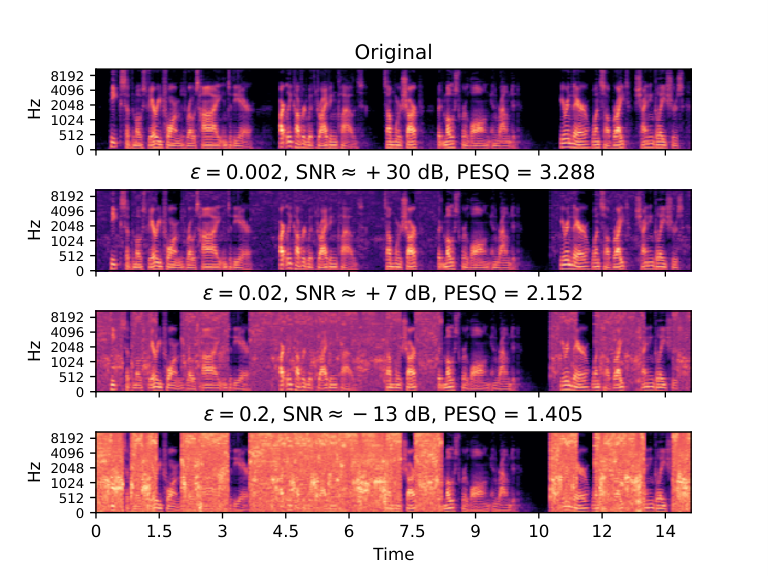
Figure 4 shows the mel-spectrograms of a randomly chosen utterance for different attacks at varying values. Here, for exploratory analysis, we increase beyond the range specified in our experiments described in the main text. We can see that for both FGSM and PGD, the noise is visible in the mel-spectrogram for . The signal becomes extremely noisy for (SNR drops below dB, and PESQ score ). On the other hand, for Carlini attack, the noise is almost invisible at and , as also evident from the high SNR values and PESQ scores. The noise becomes somewhat visible at where the SNR drops to dB, and the PESQ score becomes .
Appendix B Similarity in misclassification for different attacks
We investigate whether different attack algorithms force the model to misclassify a particular input utterance as the same (wrong) speaker. This could possibly reveal similarity between different attack algorithms. Figure 5 shows the fraction of similarity (i.e., average number of matches) between the wrong predictions made by the model for different attacks. As evident, wrong predictions for Carlini and Carlini attacks are very similar ( similarity for all the values), possibly because the inherent strategy of the Carlini attack remains the same in the two variants. The similarity between FGSM and the two Carlini attacks is also noticeable. More interestingly, the similarity scores tend to decrease when increases. We hypothesize that a low constrains the attack algorithm with a smaller space for perturbation, and hence, the model generally tends to wrongly predict the closest class (one that causes the most confusion). On the other hand, a high opens up a lot more allowed space for the perturbation, and hence, the similarity between the wrong predictions tends to decrease.