Stroboscopic two-stroke quantum heat engines

The heat stroke is depicted in Fig. 1(a). The working fluid (henceforth referred to as “the system”) is composed of $N$ sites, each with dimension $d_{i}$ and local Hamiltonians $H_{i}$. The $N$ sites are initially prepared in an arbitrary state $\rho_{S}$, which need not be a product. During the heat stroke, the sites do not interact in any way (although the state $\rho_{S}$ may very well be non-local). Each heat stroke is characterized by the interaction with two baths, $C$ and $H$, at the boundaries. The baths are described by iid ancillas, each with local Hamiltonian $H_{x}$ and prepared in thermal states $\rho_{x}=e^{-H_{x}/T_{x}}/Z_{x}$ (with $x=C,H$) at different temperatures $T_{C}$ and $T_{H}$ (for concreteness, we set $T_{C}<T_{H}$). The interaction Hamiltonian $V_{C}$ of the left bath has support only between $C$ and subsystem $S_{1}$, while $V_{H}$ has support on $S_{N}$ and $H$. This interaction is characterized by the global unitary

where $U_{q}=e^{-iH_{q}\tau_{q}}$, $\tau_{q}$ is the duration of the stroke and $H_{q}=\sum_{i=1}^{N}H_{i}+H_{C}+H_{H}+V_{C}+V_{H}$.

The main advantage of the collisional model approach is the ability to properly account for all changes in energy in both system and baths. We define heat as minus the change in energy of the ancillas,

where $\tilde{\rho}_{x}$ is the reduced state of $C$ or $H$ after the map (1). In general, however, this will not equal the change in energy of the system. The reason is that turning the interactions $V_{x}$ on and off will, in general, have an associated energy cost, called the “on/off work” De Chiara et al. 2018. In fact, energy conservation for each individual stroke implies that

where $\Delta V_{x}=\text{tr}\big\{V_{x}(\tilde{\rho}_{CS\!H}-\rho_{C}\rho_{S}\rho_{H})\big\}$. The on/off work is thus associated with energy that stays “trapped” in the interactions $V_{x}$.

The condition required for the on/off work to be zero is called strict energy conservation and reads

To make the paper more self-contained, we provide a simple proof of this in appendix A. In the language of resource theories, Eq. (5) means that the map (1) is a combination of two thermal operations Horodecki and Oppenheim 2013; Brandão et al. 2013; Brandão et al. 2015, one acting on site 1 and the other on site $N$. When (5) is satisfied, all energy leaving the system must enter the baths and vice-versa. As a consequence, the heat (2) may be equivalently defined as

which can now be computed solely from knowledge of the reduced state of the system.

A popular choice of interactions are those which have the form

where $L_{k}$ is an operator acting only on subsystem $1$ and $A_{k}$ are operators acting on $C$. A similar definition holds for the interaction $V_{H}$ between $H$ and site $N$. The condition (5) can be fulfilled in this case whenever the $\{L_{k}\}$ and $\{A_{k}\}$ are eigenoperators of $H_{1}$ and $H_{C}$; that is, if they satisfy $[H_{S},L_{k}]=-\omega_{k}L_{k}$ and $[H_{E},A_{k}]=-\omega_{k}A_{k}$, for the same set of frequencies $\{\omega_{k}\}$. In this case one usually says that $C$ and $1$ are resonant, meaning that all energy that leaves one enters the other.

We will not assume that the interaction is necessarily of the form (7), but we will from now on assume that strict energy conservation (5) is satisfied. As a consequence $W_{x}^{\text{on/off}}\equiv 0$ and therefore the change in energy of the system during the heat stroke can unambiguously be associated to heat flowing to and from the reservoirs. Finally, we also mention that in the end of the heat stroke, the reservoir ancillas are discarded and never participate again in the dynamics. This is another convenience of collisional models: since they are subsequently discarded, one can make any desired measurements in the ancillas, without having to worry about a possible measurement backaction Santos et al. 2020.

In a similar fashion, we now characterize the work stroke (Fig. 1(b)). The system is now isolated from the rest of the world and its subsystems are put to interact by means of an interaction Hamiltonian $\mathcal{V}_{S}=\sum_{i}V_{i,i+1}$, which is turned on only during the work stroke. The system will therefore evolve according to

where $U_{w}=e^{-iH_{w}\tau_{w}}$, $H_{w}=\sum_{i=1}^{N}H_{i}+\mathcal{V}_{S}$ and $\tau_{w}$ is the duration of the work stroke.

During this stroke, by turning on $\mathcal{V}_{S}$, currents are allowed to flow through the system (which will eventually flow to the reservoirs in the next stroke). The work cost associated to this is simply the on/off work of turning $\mathcal{V}_{S}$ on and off; viz.,

Work is defined as positive when energy leaves the system (i.e. work is extracted), while the heats $\mathcal{Q}_{x}$ in Eq. (6) are positive when energy enters the system.

One can also offer the following alternative justification for Eq. (9) De Chiara et al. 2018; Pereira 2018. Strictly speaking, $\mathcal{W}$ is associated with turning on and off the interaction $\mathcal{V}_{S}$. The system Hamiltonian should thus be taken to be time-dependent, of the form

where $\lambda(t)$ is a boxcar function, taking the value 1 in a window of time $\tau_{w}$. Focusing only on a single stroke, the work can then be defined using the standard statistical mechanics expression

Since the only time-dependence is in the boxcar $\lambda(t)$ (whose derivative is a pair of $\delta$ functions), one then readily finds that $\mathcal{W}$ is given precisely by Eq. (9).

The result of sewing together the two strokes is a cycle with period $\tau=\tau_{q}+\tau_{w}$. We let $\rho_{S}^{n}$ denote the state of the system after the $n$-th cycle. Combining Eqs. (1) and (8) one then finds that $\rho_{S}^{n}$ will evolve stroboscopically according to

for $n\in\mathbb{Z}$. The notation $\tilde{\rho}_{S}^{n}$ is used to denote the intermediate state, in between the two strokes.

The heat and work in each stroke will be denoted by $\mathcal{Q}_{x}^{n}$ and $\mathcal{W}^{n}$. They are readily computed from Eqs. (6) and (9) respectively. The first law for the system thus becomes

where $\Delta E_{n}=\text{tr}\big\{(\sum_{i}H_{i})(\rho_{S}^{n+1}-\rho_{S}^{n})\big\}$ is the change in energy of the system during stroke $n$. Since the energy is a function of state, $\Delta E_{n}$ can simply be written as the difference between the average energies at each stroke; the same, of course, is not true for $\mathcal{Q}_{x}^{n}$ and $\mathcal{W}^{n}$.

Similarly, one may also write down the 2nd law. Entropy is only produced during the heat stroke, so that the 2nd law can be written as Strasberg et al. 2017

where $S(\rho)=-\text{tr}\{\rho\text{ln}\rho\}$ is the von Neumann entropy. The positivity of $\Sigma^{n}$ can be readily proven, for instance, by writing it in terms of the mutual information developed between system and ancilla Esposito et al. 2010; Timpanaro et al. 2020. In this sense, it is also worth mentioning that this result holds even in the presence of on/off work in the heat stroke, provided $\mathcal{Q}_{x}$ is associated with the change in energy of the ancillas Timpanaro et al. 2020.

Repeated application of Eq. (11) will eventually take the system towards a limit cycle $\rho_{S}^{*}$, which is the solution of

The limit cycle is the stroboscopic analog of a non-equilibrium steady-state. Crucially, $\rho_{S}^{*}$ is a fixed point only of the joint map $\mathcal{E}_{w}\circ\mathcal{E}_{q}$, not the individual ones. In the limit cycle the system will therefore keep alternating between $\rho_{S}^{*}$ and $\tilde{\rho}_{S}^{*}=\mathcal{E}_{q}(\rho_{S}^{*})$, as depicted in Fig. 2.

In the limit cycle, the first law (12) simplifies to

meaning that the total heat flux during the heat stroke is converted into a net work at the work stroke. Similarly, the second law (13) becomes

In the standard thermodynamic scenario, the two terms on the RHS are associated with a flow of entropy to each side. Thus, in the limit cycle, all entropy produced in the process flows to the environment (because the entropy of the system itself no longer changes).

A special feature of the limit-cycle in two-stroke engines is that, as illustrated in Fig. 2, the state of the system bounces back and forth between only two states $\rho_{S}^{*}$ and $\tilde{\rho}_{S}^{*}$. The expressions for the heat and work, Eqs. (6) and (9) thus simplify to

But the energy of the internal sites, $i=2,\ldots,N-1$, do not change during the heat stroke. As a consequence,

Thus, when the system reaches the limit cycle, the energies of all internal sites no longer change, neither in the heat nor the work strokes. The thermodynamic output is therefore completely determined by the changes in the internal energies of the boundary sites. This is a rather peculiar feature.

In this section we discuss the connections between our framework and two other scenarios that are frequently studied in the literature. First, our framework can be viewed as a generalization of the SWAP engine introduced in Allahverdyan et al. 2010; Campisi 2014; Uzdin and Kosloff 2014; Campisi et al. 2015; Guarnieri et al. 2019. The engine consists of two non-resonant qubits. The heat stroke is exactly as described above, except that one assumes full thermalization; that is, the map (1) thermalizes 1 to $T_{C}$ and 2 to $T_{H}$. The work stroke is also defined in a similar way, but the unitary is now taken to be a full SWAP between the two qubits; i.e, $U_{\text{SWAP}}=\frac{1}{2}(1+\sigma_{x}^{1}\sigma_{x}^{2}+\sigma_{y}^{1}\sigma_{y}^{2}+\sigma_{z}^{1}\sigma_{z}^{2})$, where $\sigma_{\alpha}^{i}$ are Pauli matrices of the two qubits.

Compared to the SWAP engine Allahverdyan et al. 2010; Campisi 2014; Uzdin and Kosloff 2014; Campisi et al. 2015; Guarnieri et al. 2019, our scenario encompasses arbitrary Hilbert spaces for systems and ancillas, as well as arbitrary unitaries. The use of more general Hilbert spaces allows one to explore quantum chains made up of generic $d$-level sites, as well as more exotic chain geometries. And the use of arbitrary unitaries allows one to consider only partial thermalization and therefore study finite-time engines and transient effects.

Next, we compare our framework to a continuous-time scenario. If the duration of the heat and work strokes are sufficiently small, one may in principle move to a continuous time description by defining $\rho_{S}(t)=(\rho_{S}^{n+1}-\rho_{S}^{n})/\tau$, where $\tau=\tau_{q}+\tau_{w}$ and $t=n\tau$. Provided the changes within the strokes are small, for small $\tau$ the evolution of $\rho_{S}(t)$ will in general become smooth, described in terms of a master equation Strasberg et al. 2017. A detailed comparison, which also includes 4-stroke engines, was done in Ref. Uzdin et al. 2015. In fact, a calculation identical to the one performed in Barra 2015; De Chiara et al. 2018; Pereira 2018, shows that the continuous-time limit of our two-stroke engine is the so-called Local Master Equation (LME) (also called boundary driven master equation), where Lindblad jump operators act only on the end-sites.

The physical interpretation of this continuous-time limit is identical to that used in classical thermodynamics. A car engine, for instance, is stroke based. However, each cycle lasts for a very short period of time so that, in a coarse-grained time scale, one can view it as operating in continuous-time. Similarly, LMEs can be viewed as the continuous-time limit of our two-stroke engine.

A special feature of the SWAP engine Allahverdyan et al. 2010; Campisi 2014; Uzdin and Kosloff 2014; Campisi et al. 2015 is that, despite having only two strokes, its efficiency is always given by the Otto efficiency. It turns out that there is a broader class of problems for which this is also true. In fact, as we now show, this will be the case whenever the internal interaction $\mathcal{V}_{S}$ has the form

where the $L_{i}$ are eigenoperators of each site Hamiltonian $H_{i}$. That is, $[H_{i},L_{i}]=-\omega_{i}L_{i}$. The transition frequency $\omega_{i}$ may in general be different from one site to another. However, it is necessary for (22) to contain only one jump operator for each site. Mixing multiple jump operators doesn’t work. We also notice that the local Hamiltonians $H_{i}$ can still be absolutely general, each with arbitrary dimensions and internal structures.

To prove this claim, we focus on the work stroke. Using Heisenberg’s equation, the evolution of each local site Hamiltonian will be given by

Integrating over the duration $\tau_{w}$ of the work stroke, we find that

where

For simplicity, we assumed the system was already in the limit-cycle. This result holds for all internal sites $i=2,\ldots,N-1$. It can also hold for the boundaries, provided we define $J_{0,1}=J_{N,N+1}=0$.

Because of the limit-cycle property (21), however, one must have

As a consequence, using the definitions of $\mathcal{Q}_{C}^{*}$ and $\mathcal{Q}_{H}^{*}$ in Eqs. (17) and (18), one finds that

On the other hand, if there was no work, from Eqs. (19) and (21) it is clear to note that $\mathcal{Q}_{C}=-\mathcal{Q}_{H}$. Considering nonzero work, Eq. (25) establishes a direct relation between the two heats in the limit-cycle. Because of the 1st law, Eq. (15), this also fixes $\mathcal{W}^{*}$ in terms of $\mathcal{Q}_{H}^{*}$.

The efficiency is defined as

where we also used the 1st law (15). Substituting (25) then finally leads to

which is the Otto efficiency Callen 1985. The engine’s efficiency is therefore completely determined by the transition frequencies of the first and last sites. Note that these frequencies are established by the jump operators $L_{i}$ in Eq. (22): the local Hamiltonians $H_{i}$ will in general have several transition frequencies. But the interaction $\mathcal{V}_{S}$ in (22) selects a specific $\omega_{i}$ for each site. We also call attention to the fact that (27) is independent of the cycle duration $\tau$. As a consequence, one may tune $\tau$ to optimize the output power, without having to bother about a decrease in efficiency.

Eq. (25) also has an important consequence for the 2nd law. Substituting it in Eq. (16), one finds that

Since $\Sigma^{*}\geq 0$ by construction, it follows from this result that $\mathcal{Q}_{H}^{*}$ must have the same sign as the pre-factor. Thus, what determines the direction of heat flow is not the gradient of temperature, but the “gradient of $\omega/T$”. That is, the difference between $\omega_{1}/T_{C}$ and $\omega_{N}/T_{H}$. This is so because there is work involved, so that the standard Clausius statement, saying that heat must flow from hot to cold, does not apply (since it assumes there is no work involved). This result generalizes a discussion in De Chiara et al. 2018 about possible violations of the 2nd law in LMEs Levy and Kosloff 2014. Refs. De Chiara et al. 2018; Levy and Kosloff 2014 dealt with bosonic chains (fermionic chains are mathematically equivalent). In that case, what mattered for the heat flow direction was the difference in the Bose-Einstein (Fermi-Dirac) occupations. Eq. (28) shows that this is more general. All it requires is an eigenoperator-type interaction of the form (22). As an interesting sanity check, we may verify what happens when the Otto efficiency coincides with the Carnot efficiency. That is, when the frequencies are chosen so that $\omega_{1}/\omega_{N}=T_{C}/T_{H}$. In this case we see from Eq. (28) that $\Sigma^{*}=0$, which agrees with the idea of the Carnot cycle being reversible. In the SWAP engine, the output power is also identically zero in this limit, so that even though the engine operates reversibly, nothing is extracted from it. It is unclear to us whether a similar result should also hold for all 2-stroke engines encompassed in our framework.

We begin by considering a system composed of two non-resonant qubits, each with local Hamiltonian $H_{i}=\omega_{i}\sigma_{z}^{i}/2$. The ancillas for the two baths are taken to be resonant with their respective qubits. That is $H_{C}=\omega_{C}\sigma_{z}^{C}/2$ and $H_{H}=\omega_{H}\sigma_{z}^{H}/2$ with $\omega_{C}=\omega_{1}$ and $\omega_{H}=\omega_{2}$. The initial thermal states $\rho_{x}$ of the two baths are thus characterized only by the Fermi-Dirac population, $f_{x}=(e^{\beta_{x}\omega_{x}}+1)^{-1}$. We take all interactions to be of the form [c.f. Eqs. (7) or (22)]

By this we mean the internal system interaction $\mathcal{V}_{S}=\vartheta_{12}$ as well as the system-bath interactions $V_{C}=\vartheta_{1,C}$ and $V_{H}=\vartheta_{2,H}$. The conditions that $1C$ and $2H$ are resonant then ensures that there is no on/off work during the heat stroke. Moreover, the fact that 1 and 2 are not resonant is precisely the source of work during the work stroke.

Instead of working with the full map (11), it turns out that in this case one can write down a closed system of equations for only a handful of observables for the system qubits $1$ and $2$. We define the $c$-number variables $Z_{i}^{n}=\langle\sigma_{z}^{i}\rangle_{n}$ ($i=1,2$), as well as the correlations $S^{n}=\langle\sigma_{+}^{1}\sigma_{-}^{2}+\sigma_{-}^{1}\sigma_{+}^{2}\rangle_{n}$ and $A^{n}=i\langle\sigma_{+}^{1}\sigma_{-}^{2}-\sigma_{-}^{1}\sigma_{+}^{2}\rangle_{n}$ [where $\langle\ldots\rangle_{n}=\text{tr}(\ldots\rho_{S}^{n})$]. From these variables, the heats are computed as $\mathcal{Q}_{x}^{n}=\omega_{x}(\tilde{Z}_{x}^{n}-Z_{x}^{n})/2$ while the work is $\mathcal{W}^{n}=-\sum_{i=1,2}\omega_{i}(Z_{i}^{n+1}-\tilde{Z}_{i}^{n})/2$.

Using the map (1), a straightforward calculation shows that during the heat stroke these variables will evolve according to

where $Z_{i}^{\text{th}}=(2f_{i}-1)$ is the equilibrium spin component of each qubit in the temperature of its respective bath. We also defined the parameters $p=\cos^{2}[(\omega_{1}-\omega_{2})\tau_{q}]$ and $\lambda=(1-\cos(2g\tau_{q}))/2$, where $g=g_{CH}=g_{C,1}=g_{H,2}$ is the interaction parameter for the system-bath interactions [Eq. (29)], which we assume are the same for both.

These equations help to clarify the role of different parameters, as well as the relevant time scales. The system-bath interactions $1C$ and $2H$ are nothing but partial SWAPs with strength $\lambda$, with $\lambda=1$ meaning full thermalization (as is clear from Eq. (30)). The parameter $p$, on the other hand, represents a “transfer” from $S$ to $A$, which is associated to the mismatch $\omega_{1}-\omega_{2}$ between the two qubits and is independent of $g_{CH}$. Notice also that since the system qubits do not interact during the heat stroke, if initially $S^{n}=A^{n}=0$, then the same will be true of $\tilde{S}^{n}$ and $\tilde{A}^{n}$; that is to say, the heat stroke cannot create correlations between the two qubits, only destroy them.

Similarly, during the work stroke defined by the map (8), the variables $(Z_{1},Z_{2},S,A)$ are found to evolve according to

where we introduced the auxiliary parameters $\eta=(2g^{2}/\omega_{r}^{2})[1-\text{cos}(\omega_{r}\tau_{w})]$ (not the be confused with the efficiency), $\xi=(g/\omega_{r})\sin(\omega_{r}\tau_{w})$ and $\tan(\theta)=(\omega_{1}-\omega_{2})/2g$, with $\omega_{r}:=\sqrt{4g^{2}+(\omega_{1}-\omega_{2})^{2}}$ being the Rabi frequency. These parameters are related according to $\xi^{2}=\eta(1-\eta\sec^{2}\theta)$.

The parameter $\eta$ plays a similar role to $\lambda$ in Eqs. (30)-(32), quantifying the strength of the internal system coupling. Unlike $\lambda$, however, the parameter $\eta$ can never implement a full SWAP; that is, one can never have $\eta=1$. In fact, $\eta<\cos^{2}\theta$. This occurs because the two qubits are not resonant; if they were, then we would have $\omega_{r}=2g$ and the limit $\eta\to 1$ would be reachable. The parameter $\theta$ plays a similar role to $p$, in the sense that it is related to the detuning between the two qubits, and vanishes if they are resonant. Unlike $p$, however, $\theta$ is independent of the interaction time.

The work stroke, as can be seen, involves not only a partial SWAP in the local populations $Z_{1}$ and $Z_{2}$, but also mixes the populations and correlations. This mixing is related in a not so intuitive way to both parameters $\xi$ and $\theta$. In fact, even in the resonant case, where $\theta=0$, this mixing still remains because $\xi$ continues to be non-zero.

The two systems of equations, (30)-(32) and (33)-(36) form a simple set of vector difference equations for the vector $\bm{x}_{n}=(Z_{1}^{n},Z_{2}^{n},S^{n},A^{n})$, which can be written as

where the $4\times 4$ matrices $J$ and $D$, as well as the vector $S$, can be readily read from Eqs. (30)-(36). For instance, the matrix $S$ is associated only with the terms $\lambda S_{i}^{\text{th}}$ in Eq. (30) and therefore reads $S=\lambda\,\text{diag}(2f_{C}-1,2f_{H}-1,0,0)$.

The general solution of this type of difference equation reads

We therefore see that the bulk of the dynamics is governed by the matrix $DJ$. In addition, one may also determine the steady-state by setting $\bm{x}_{n}=\bm{x}_{n+1}=\bm{x}^{*}$ in Eq. (38). As a result one finds

The full expression is somewhat cumbersome, but can nonetheless be computed analytically using e.g. Mathematica.

An illustrative example of the evolution of the $\bm{x}_{n}$ and $\tilde{\bm{x}}_{n}$ is shown in Fig.(3). These plots clearly exhibit the convergence towards the steady state, where the system keeps bouncing back and forth between $\bm{x}^{*}$ and $\tilde{\bm{x}}^{*}$, similarly to a piston going up and down. From the entries of $\bm{x}_{n}$ and $\tilde{\bm{x}}_{n}$, one readily computes the relevant thermodynamic variables $\mathcal{Q}_{x}=\omega_{x}(\tilde{Z}_{x}^{n}-Z_{x}^{n})/2$ and $\mathcal{W}=-\sum_{i=1,2}\omega_{i}(Z_{i}^{n+1}-\tilde{Z}_{i}^{n})/2$. The results are shown in Fig. 4. The thermodynamic variables tend to non-zero values, as indicated by the numbers in the figure. Since the work is positive (extraction), this corresponds to a heat engine configuration. We see that, initially, the work is very small, while the heat losses are significant. This, of course, depends on the initial conditions. But they reflect well the typical adaptation of the heat engine towards the limit-cycle operation. This therefore serves to illustrate that thermodynamically relevant quantities, such as the net output work in the limit-cycle, may behave in significantly different ways, in the transient and the limit cycle.

Next we address the relaxation time, which is associated with the number of cycles that the engine must run before reaching the limit-cycle. This is related to the eigenvalues of the matrix $DJ$, which is the basic matrix governing the dynamics of $\bm{x}_{n}$ in Eq. (39). The dynamics depends on powers of $DJ$. Stability thus requires that its eigenvalues lie within the unit circle. Small eigenvalues are quickly suppressed when taking it to the power $n$. Thus, the longest relaxation time of the system will be described by the largest eigenvalue (in magnitude) of $DJ$:

The closer $\mu$ is to unity, the longer the system takes to relax to the limit-cycle.

From Eqs. (30)-(32), one notices that all entries in the matrix $J$ depend equally on $1-\lambda$. Hence, $\mu\propto 1-\lambda$. It turns out, however, that this is an exact equality. As may be verified from the clumsy, but exact, formulas for $D$ and $J$, the matrix $DJ/(1-\lambda)$ has an eigenvalue $1$. And so, by stability, all others must necessarily have magnitude below 1. Hence, we conclude that the longest relaxation time (41) is exactly $\mu=1-\lambda$. That is, the relaxation is fully dictated by the heat stroke, as one might intuitively expect.

Finally, we turn to the output power,

Our system falls under the category of Sec. II.6 and therefore its efficiency is always given by the Otto formula (27). The output power, however, is not fixed but depends sensibly on all parameters. Using the difference equations approach described above, it is possible to write down an explicit, and not too cumbersome, formula for $\mathcal{W}^{*}$:

The output power depends on the stroke times $\tau_{q}$ and $\tau_{w}$, which are also contained implicitly in the parameters $\lambda$, $p$ and $\eta$ above.

Eq. (43) provides a clear illustration of the physics behind each parameter involved in the model. First, we see that $\mathcal{W}^{*}$ depends on $(f_{C}-f_{H})(\omega_{1}-\omega_{2})$. The Fermi function $(e^{x}+1)^{-1}$ is monotonically decreasing in $x$. Thus, if we fix $T_{C}<T_{H}$, the output work will be positive when $f_{c}<f_{H}$ and $\omega_{1}<\omega_{2}$, which establishes the operating interval for the machine to function as an engine:

It is also interesting to analyze some particular cases of (43). First, for full thermalization ($\lambda\to 1$), it reduces to

This is close to the result of the SWAP engine Allahverdyan et al. 2010; Campisi 2014; Uzdin and Kosloff 2014; Campisi et al. 2015; Guarnieri et al. 2019. The difference is that the SWAP engine assumes a unitary stroke implementing a full SWAP, so that $\eta=1$. In our case, we are assuming $\eta$ stems from a microscopic interaction so, as discussed, this limit cannot be reached. Similar infinitesimal expansions can also be performed for the other parameters. In particular, the structure of the numerator in Eq. (43) shows the leading order contributions of $\lambda$, $\eta$ and $(\omega_{1}-\omega_{2})$ will all be linear. This, of course, is physically consistent, since the work output is meant to vanish if (i) the internal system coupling vanishes, (ii) the coupling to the baths vanish and (iii) the two system qubits are resonant. The latter, in particular, occurs because in this limit the interaction becomes a thermal operation.

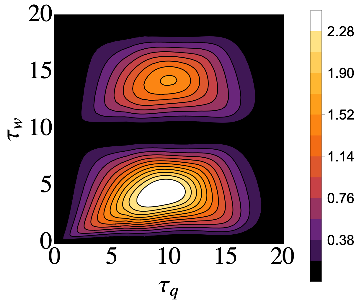
Eq. (43) makes it efficient to optimize the output power by tweaking the system parameters. To illustrate this, in Fig. 5 we plot $\mathcal{P}^{*}$ as a function of the interaction times $\tau_{q}$ and $\tau_{w}$, of each stroke. The dependence on these parameters is not trivial. Part of it is oscillatory, through their dependence on the parameters $\lambda$, $p$ and $\eta$. This is clearly observed in the figure. But, in addition, $\mathcal{P}^{*}$ is also inversely proportional to $\tau_{q}+\tau_{w}$. For very large $\tau_{q}$ and $\tau_{w}$, this will cause $\mathcal{P}^{*}$ to decreases as one moves across the diagonal in the figure. But for intermediate values, increases may be observed as well.

The results for the 2-qubit engine resemble, in many aspects, the SWAP engine Allahverdyan et al. 2010; Campisi 2014; Uzdin and Kosloff 2014; Campisi et al. 2015; Guarnieri et al. 2019. The difference is that now the engine is operated in finite time, which therefore introduces multiple new features. The 2-stroke framework developed in this paper, however, is not restricted to this simple scenario. To illustrate this, we now consider an engine whose working fluid is a spin chain of $N$ sites, while the reservoirs are still single spins. For simplicity, we focus on linear chains, although this is not at all a restriction. Each spin has, as before, a local Hamiltonian $H_{i}=\tfrac{1}{2}\omega_{i}\sigma_{i}^{z}$. The system-bath interactions $1C$ and $NH$ are still of the form (29), with the ancillas resonant with their respective sites (so as to ensure there is no on/off work). The internal interaction Hamiltonian however, is now taken more generally to be

The total Hamiltonian during the work stroke will thus be $H=\sum_{i}H_{i}+\mathcal{V}_{S}$. We focus on small chains ($N\leq 6$), for which the problem can be treated using exact diagonalization. Moreover, we analyze two particular cases: (i) XX model $J_{x}=J_{y}=J$, $J_{z}=0$ and (ii) XXZ chain, $J_{x}=J_{y}=J$, $J_{z}=J\Delta$. The results for each case are summarized in Fig. 6. Images (a)-(c) (left column) are for the XX and (d)-(f) (right) for the XXZ. Moreover, (a) and (d) show the transient dynamics of of $\mathcal{Q}_{C}^{n}$, $\mathcal{Q}_{H}^{n}$, while (b) and (e) show that of $\mathcal{W}^{n}$. Finally, (c) and (f) show the limit cycle output power as a function of $\lambda$ (which is equivalent to $\tau_{q}$).

We start by analyzing the XX model (Fig. 6(a)-(c)). It can be seen that both the stationary values of heat and work are independent of the size of the chain. The extracted power in the limit cycle, on the other hand, is weakly affected by $N$ and likewise the value of $\lambda$ for which the power is maximum. These results are consistent with the fact that, by making the changes $\sigma_{x}\rightarrow\sigma_{+}+\sigma_{-}$ and $\sigma_{y}\rightarrow-i(\sigma_{+}-\sigma_{-})$, the interaction Hamiltonian can be written in the same form as Eq. (29) and therefore similar results to the $N=2$ case would be expected. A similarly weak dependence of the XX model in the chain size $N$ has also been observed in De Chiara et al. 2018, for a non-interacting bosonic chain. This, we believe, is related to the non-interacting nature of these models. For instance, it is known that the XX model presents ballistic transport, whereas the XXZ does not.

Now we pass to the XXZ chain. In contrast with the XX model, the XXZ spin chain shows a significant variation for the heat, work and power. In Fig. 6(d), we note that $\mathcal{Q}_{H}^{*}$ decreases for increasing $N$ and then, as a result, $\mathcal{W}^{*}$ (Fig. 6(e)) also gets lower when enlarging the spin chain. A notable change in the extracted power is also observed (Fig. 6(f)). The maximum value of $\mathcal{P}^{*}$ with respect to $\lambda$ gets lower for increasing $N$ and the $\lambda$ for which the extracted power is maximum is slightly shifted to the right.

References

- Binder et al. (2018) F. Binder, L. A. Correa, C. Gogolin, J. Anders, and G. Adesso, Thermodynamics in the Quantum Regime: Fundamental Aspects and New Directions (Springer, 2018).
- Geva and Kosloff (1992) E. Geva and R. Kosloff, J. Chem. Phys. 96, 3054 (1992).
- Kosloff and Feldmann (2002) R. Kosloff and T. Feldmann, Phys. Rev. E - Stat. Physics, Plasmas, Fluids, Relat. Interdiscip. Top. 65, 4 (2002).
- Quan et al. (2007) H. T. Quan, Y. X. Liu, C. P. Sun, and F. Nori, Physical Review E - Statistical, Nonlinear, and Soft Matter Physics 76, 1 (2007), arXiv:0611275 [quant-ph] .
- Campisi et al. (2015) M. Campisi, J. Pekola, and R. Fazio, New J. Phys. 17, 1 (2015), arXiv:arXiv:1412.0898v1 .
- Kosloff and Rezek (2017) R. Kosloff and Y. Rezek, “The quantum harmonic otto cycle,” (2017), arXiv:1612.03582 .
- Scopa et al. (2019) S. Scopa, G. T. Landi, A. Hammoumi, and D. Karevski, Phys. Rev. A 99, 1 (2019), arXiv:1811.05490 .
- Chen et al. (2019) J. F. Chen, C. P. Sun, and H. Dong, Phys. Rev. E 100, 1 (2019), arXiv:1907.11567 .
- Linden et al. (2010) N. Linden, S. Popescu, and P. Skrzypczyk, Phys. Rev. Lett. 105, 1 (2010), arXiv:0908.2076 .
- Kosloff and Levy (2014) R. Kosloff and A. Levy, Annu. Rev. Phys. Chem. 65, 365 (2014), arXiv:1310.0683 .
- Müller (2018) M. P. Müller, Phys. Rev. X 8, 41051 (2018), arXiv:1707.03451 .
- De Chiara et al. (2018) G. De Chiara, G. Landi, A. Hewgill, B. Reid, A. Ferraro, A. J. Roncaglia, and M. Antezza, New J. Phys. 20 (2018), 10.1088/1367-2630/aaecee, arXiv:1808.10450 .
- Clivaz et al. (2019) F. Clivaz, R. Silva, G. Haack, J. B. Brask, N. Brunner, and M. Huber, Physical Review Letters 123, 1 (2019), arXiv:1903.04970 .
- Mitchison (2019) M. T. Mitchison, Contemporary Physics 60, 164 (2019), arXiv:1902.02672 .
- Insinga et al. (2018) A. Insinga, B. Andresen, P. Salamon, and R. Kosloff, Physical Review E 97, 62153 (2018), arXiv:1801.01296 .
- Josefsson and Leijnse (2020) M. Josefsson and M. Leijnse, Physical Review B 101, 81408 (2020), arXiv:1912.04637 .
- Gherardini et al. (2020) S. Gherardini, F. Campaioli, F. Caruso, and F. C. Binder, Phys. Rev. Res. 2, 1 (2020), arXiv:1910.02458 .
- Rezek and Kosloff (2006) Y. Rezek and R. Kosloff, New J. Phys. 8, 1 (2006), arXiv:0601006 [quant-ph] .
- Kim et al. (2011) S. W. Kim, T. Sagawa, S. De Liberato, and M. Ueda, Physical Review Letters 106, 1 (2011), arXiv:1006.1471 .
- Gelbwaser-Klimovsky et al. (2013) D. Gelbwaser-Klimovsky, R. Alicki, and G. Kurizki, Phys. Rev. E 87, 012140 (2013).
- Scovil and Schulz-Dubois (1959) H. E. Scovil and E. O. Schulz-Dubois, Phys. Rev. Lett. 2, 262 (1959).
- Barra (2015) F. Barra, Scientific Reports 5, 14873 (2015), arXiv:1509.04223 .
- Pereira (2018) E. Pereira, Physical Review E 97, 022115 (2018).
- Sparaciari et al. (2017) C. Sparaciari, J. Oppenheim, and T. Fritz, Phys. Rev. A 96, 052112 (2017).
- Brandão et al. (2013) F. G. S. L. Brandão, M. Horodecki, J. Oppenheim, J. M. Renes, and R. W. Spekkens, Phys. Rev. Lett. 111, 250404 (2013).
- Gour et al. (2015) G. Gour, M. P. Müller, V. Narasimhachar, R. W. Spekkens, and N. Yunger Halpern, Physics Reports 583, 1 (2015), the resource theory of informational nonequilibrium in thermodynamics.
- Scarani et al. (2002) V. Scarani, M. Ziman, P. Štelmachovič, N. Gisin, V. Bužek, and V. Bužek, Phys. Rev. Lett. 88, 979051 (2002), arXiv:0110088 [quant-ph] .
- Strasberg and Esposito (2019) P. Strasberg and M. Esposito, Phys. Rev. E 99 (2019), 10.1103/PhysRevE.99.012120, arXiv:arXiv:1806.09101v3 .
- Landi et al. (2014) G. T. Landi, E. Novais, M. J. De Oliveira, and D. Karevski, Phys. Rev. E - Stat. Nonlinear, Soft Matter Phys. 90, 1 (2014).
- Giovannetti and Palma (2012) V. Giovannetti and G. M. Palma, Phys. Rev. Lett. 108, 040401 (2012).
- Ziman et al. (2002) M. Ziman, P. Štelmachovič, V. Bužek, M. Hillery, V. Scarani, and N. Gisin, Phys. Rev. A 65, 042105 (2002).
- Rodrigues et al. (2019) F. L. S. Rodrigues, G. De Chiara, M. Paternostro, and G. T. Landi, Phys. Rev. Lett. 123, 140601 (2019), arXiv:1906.08203 .
- Allahverdyan et al. (2010) A. E. Allahverdyan, K. Hovhannisyan, and G. Mahler, Phys. Rev. E 81, 051129 (2010).
- Campisi (2014) M. Campisi, Journal of Physics A: Mathematical and Theoretical 47, 245001 (2014).
- Uzdin and Kosloff (2014) R. Uzdin and R. Kosloff, New Journal of Physics 16, 095003 (2014).
- Guarnieri et al. (2019) G. Guarnieri, G. T. Landi, S. R. Clark, and J. Goold, Physical Review Research 1, 1 (2019), arXiv:1901.10428 .
- Horodecki and Oppenheim (2013) M. Horodecki and J. Oppenheim, Nat. Commun. 4 (2013), 10.1038/ncomms3059, arXiv:1111.3834 .
- Brandão et al. (2015) F. Brandão, M. Horodecki, N. Ng, J. Oppenheim, and S. Wehner, Proc. Natl. Acad. Sci. U. S. A. 112, 3275 (2015), arXiv:1305.5278 .
- Santos et al. (2020) J. P. Santos, A. M. Timpanaro, and G. T. Landi, “Joint fluctuation theorems for sequential heat exchange,” (2020), arXiv:2003.02150 [quant-ph] .
- Strasberg et al. (2017) P. Strasberg, G. Schaller, and T. Brandes, Phys. Rev. X 7, 1 (2017), arXiv:1610.01829 .
- Esposito et al. (2010) M. Esposito, K. Lindenberg, and C. Van den Broeck, New Journal of Physics 12, 013013 (2010), arXiv:0908.1125 .
- Timpanaro et al. (2020) A. M. Timpanaro, J. P. Santos, and G. T. Landi, Physical Review Letters 124, 240601 (2020), arXiv:1911.00910 .
- Uzdin et al. (2015) R. Uzdin, A. Levy, and R. Kosloff, Phys. Rev. X 5, 031044 (2015).
- Callen (1985) H. B. Callen, Thermodynamics and an introduction to thermostatistics; 2nd ed. (Wiley, New York, NY, 1985).
- Levy and Kosloff (2014) A. Levy and R. Kosloff, European Physics Letters 107, 20004 (2014), arXiv:1402.3825 .