Skeleton-based Action Recognition via Spatial and Temporal Transformer NetworksJournal: Computer Vision and Image Understanding
Abstract
Skeleton-based Human Activity Recognition has achieved great interest in recent years as skeleton data has demonstrated being robust to illumination changes, body scales, dynamic camera views, and complex background. In particular, Spatial-Temporal Graph Convolutional Networks (ST-GCN) demonstrated to be effective in learning both spatial and temporal dependencies on non-Euclidean data such as skeleton graphs. Nevertheless, an effective encoding of the latent information underlying the 3D skeleton is still an open problem, especially when it comes to extracting effective information from joint motion patterns and their correlations. In this work, we propose a novel Spatial-Temporal Transformer network (ST-TR) which models dependencies between joints using the Transformer self-attention operator. In our ST-TR model, a Spatial Self-Attention module (SSA) is used to understand intra-frame interactions between different body parts, and a Temporal Self-Attention module (TSA) to model inter-frame correlations. The two are combined in a two-stream network, whose performance is evaluated on three large-scale datasets, NTU-RGB+D 60, NTU-RGB+D 120, and Kinetics Skeleton 400, consistently improving backbone results. Compared with methods that use the same input data, the proposed ST-TR achieves state-of-the-art performance on all datasets when using joints’ coordinates as input, and results on-par with state-of-the-art when adding bones information.
MSC
41A05, 41A10, 65D05, 65D17 \KWDRepresentation Learning , Graph CNN , Self-Attention , 3D Skeleton , Action Recognition1 Introduction
Human Action Recognition is achieving increasing interest in recent years for the progress achieved in deep learning and computer vision and for the interest of its applications in human-computer interaction, eldercare and healthcare assistance, as well as video surveillance. Recent advances in 3D depth cameras such as Microsoft Kinect (Zhang 2012) and Intel RealSense (Keselman et al. 2017) sensors, and advanced human pose estimation algorithms (Cao et al. 2019) made it possible to estimate 3D skeleton coordinates quickly and accurately with cheap devices. Nevertheless, several aspects of skeleton-based action recognition still remain open (Zhang et al. 2019; Aggarwal and Ryoo 2011; Ren et al. 2020). The most widespread method to perform skeleton-based action recognition has nowadays become Graph Neural Networks (GNNs), and in particular, Graph Convolutional Networks (GCNs) since, being an efficient representation of non-Euclidean data, they are able to effectively capture spatial (intra-frame) and temporal (inter-frame) information. Models making use of GCN were first introduced in skeleton-based action recognition by Yan et al. 2018 and they are usually referred to as Spatial-Temporal Graph Convolutional Networks (ST-GCNs). These models process spatial information by operating on skeleton bone-connections along space, and temporal information by considering additional time-connections between each skeleton joint along time. Despite being proven to perform very well on skeleton data, ST-GCN models have some structural limitations, some of them already addressed by Shi et al. 2019a; Simonyan and Zisserman 2014; Cheng et al. 2020; Liu et al. 2020.
First of all, the topology of the graph representing the human body is fixed for all layers and all the actions; this may prevent the extraction of rich representations for the skeleton movements during time, especially if graph links are directed and information can only flow along a predefined path. Secondly, both Spatial and Temporal Convolution are implemented starting from a standard 2D convolution. As such, they are limited to operate in a local neighborhood, somehow restricted by the convolution kernel size. And finally, as a consequence of the previous, correlations between body joints not linked in the human skeleton, e.g., the left and right hands, are underestimated even if relevant in actions such as “clapping".

In this paper, we face all these limitations by employing a modified Transformer self-attention operator, as depicted in Figure 1. Despite being originally designed for Natural Language Processing (NLP) tasks, Transformer self-attention has shown remarkable results on a broad range of computer vision tasks, spanning from classical classification and detection (Dosovitskiy et al. 2020; Bello et al. 2019a; Wang et al. 2018; Carion et al. 2020), to more complex tasks such as those involving point clouds (Zhao et al. 2020), generative modeling (Oord et al. 2016; Parmar et al. 2018) and captioning (He et al. 2020). In our setting, the sequentiality and hierarchical structure of human skeleton sequences, as well as the flexibility of Transformer self-attention (Vaswani et al. 2017) in modeling long-range dependencies, make the Transformer a perfect solution to tackle ST-GCN weaknesses. In our work, we aim to apply Transformer to spatial-temporal skeleton-based architectures, and in particular to joints representing the human skeleton, with the goal of modeling long-range interactions within human actions both in space, through a Spatial Self-Attention (SSA) module, and time, through a Temporal Self-Attention (TSA) module. Main contributions of this paper are summarized as follows:
- 1.
We propose a novel two-stream Transformer-based model for skeleton activity recognition tasks, employing self-attention on both the spatial and the temporal dimensions
- 2.
We design a Spatial Self-Attention (SSA) module to dynamically build links between skeleton joints, representing the relationships between human body parts, conditionally on the action and independently from the natural human body structure. On the temporal dimension, we introduce a Temporal Self-Attention (TSA) module to study the dynamics of a joint along time. We made both layers publicly available for experiments replication and further use 11 1 Code at https://github.com/Chiaraplizz/ST-TR
- 3.
Our model outperforms ST-GCN (Yan et al. 2018) and A-GCN (Shi et al. 2019b) consistently improving backbone results on all datasets and achieving state-of-the-art performance when using joint information, and results on-par with state-of-the-art when bones information is used.
2 Related Works
2.1 Skeleton-based Action Recognition
Most of the early studies in skeleton-based action recognition relied on handcrafted features (Hu et al. 2015; Vemulapalli et al. 2014; Hussein et al. 2013) exploiting relative 3D rotations and translations between joints. Deep learning revolutionized activity recognition by proposing methods capable of increased robustness (Wang et al. 2019) and able to achieve unprecedented performance. Methods that fall into this category rely on different aspects of skeleton data: (1) Recurrent neural network (RNN) based methods (Lev et al. 2016; Wang and Wang 2017; Liu et al. 2017b; Du et al. 2015) leverage on the sequentiality of joint coordinates, treating input skeleton data as time series. (2) Convolutional neural network (CNN) based methods (Chéron et al. 2015; Simonyan and Zisserman 2014; Ding et al. 2017; Liu et al. 2017c; Li et al. 2017) leverage spatial information, in a complementary way to RNN-based ones. Indeed, 3D skeleton sequences are mapped into a pseudo-image, representing temporal dynamics and skeleton joints respectively in rows and columns. (3) Graph neural network (GNN) based methods (Yan et al. 2018; Li et al. 2019; Shi et al. 2019b; Shi et al. 2019a; Cheng et al. 2020; Liu et al. 2020), make use of both spatial and temporal data by exploiting information contained in the natural topological graph structure of the human skeleton. These latter methods have demonstrated to be the most expressive among the three, and among these, the first model capturing the balance between spatial and temporal dependencies has been the Spatio-Temporal Graph Convolutional Network (ST-GCN) (Yan et al. 2018).
In this work, we used ST-GCN as the baseline model; its functioning is presented in details in Section 3.2. Specifically, we propose to substitute regular graph convolutions on both space and time with the transformer self-attention operator. Cho et al. 2020 also proposed a Self-Attention Network (SAN) in which embeddings are extracted by segmenting the action sequence in temporal clips, and self-attention is applied among them in order to model long-term semantic information. However, since it applies self-attention on course-grained embeddings rather than skeleton joints, it hardly captures low-level joints’ correlations within and between frames. Instead, by applying self-attention directly on nodes in the graph, both intra- and inter-frame, we efficiently model both spatial and temporal dependencies of the skeleton sequence.
2.2 Graph Neural Networks
Geometric deep learning (Bronstein et al. 2017) refers to all emerging techniques attempting to generalize deep learning models to non-Euclidean domains such as graphs. The notion of Graph Neural Network (GNN) was initially outlined by Gori et al. 2005 and further elaborated by Scarselli et al. 2008. The intuitive idea underlying GNNs is that nodes in a graph represent objects or concepts while edges represent their relationships. Due to the success of Convolutional Neural Networks, the concept of convolution has later been generalized from grid to graph data. GNNs iteratively process the graph, each time representing nodes as the result of applying a transformation to nodes’ and their neighbors’ features. The first formulation of CNNs on graphs is due to Bruna et al. 2014, who generalized convolution to signals using a spectral construction. This approach had computational drawbacks that have been subsequently addressed by Henaff et al. 2015 and Defferrard et al. 2016. The latter has been further simplified and extended by Kipf and Welling 2017. A complementary approach is the spatial one, where graph convolution is defined as information aggregation (Micheli 2009; Niepert et al. 2016; Such et al. 2017). In this work we make use of the spectral construction proposed by Kipf and Welling 2017, whose formulation is provided in Section 3.2.
2.3 Transformers in Computer Vision
The Transformer is the leading neural model for Natural Language Processing (NLP), proposed by Vaswani et al. 2017 as an alternative to recurrent networks. It has been designed to face two key problems: (i) the processing of very long sequences, which are often intractable both for LSTMs and RNNs, and (ii) the limitations in parallelizing sentence processing, which is usually performed sequentially, word by word, in standard RNNs architectures. The Transformer follows a usual encoder-decoder structure, but it relies solely on multi-head self-attention (Vaswani et al. 2017). Recently, Transformer self-attention has been applied in many popular computer vision tasks. Wang et al. 2018 proposed a differentiable non-local operator based on self-attention, which allows to capture long-range dependencies both in space and time for a more accurate video classification. After the first attempt of Bello et al. 2019a to use self-attention as an alternative to convolutional operators, Dosovitskiy et al. 2020 proposed a Vision Transformer (ViT), which shows how Transformers can effectively replace standard convolutions on images. He et al. 2020 proposed a novel image transformer architecture for the image captioning task. Carion et al. 2020 made the first attempt to use a Transformer model to tackle detection problems, namely the Detection Transformer (DeTR). Zhao et al. 2020 proposed Point Transformer, a model which uses transformer self-attention to encode relations between point clouds, exploiting their permutation invariant nature. Other applications of Transformers in segmentation tasks (Huang et al. 2019), multi-modal tasks (Lee et al. 2020) and generative modeling (Oord et al. 2016; Parmar et al. 2018) have been recently developed, showing the potential of Transformer models on a broad range of tasks.
3 Background
In this section, Spatial-Temporal Graph Convolutional Networks (ST-GCN) by Yan et al. 2018 and the original Transformer self-attention by Vaswani et al. 2017 are summarized, being the basic blocks of the model we propose in this paper.
3.1 Skeleton Sequences Representation
Given a sequence of skeletons, we define as the number of joints representing each skeleton and as the total number of skeletons composing the sequence, also named frames in the following. In order to represent the sequence, a spatial temporal graph is built, i.e., , where represents the set of all the nodes of the graph, i.e., the body joints of the skeleton along all the time sequence, and represents the set of all the connections between nodes. consists of two subsets; the first subset is composed by the intra-skeleton connections at each time interval , for any pair of joints connected by a bone in the human skeleton. The subset of intra-skeleton connections is commonly further divided into disjoint partitions, based on some criterion (Yan et al. 2018) (e.g., distance from the center of gravity), and encoded using a set of adjacency matrices . The second subset consists of all the inter-frame connections between joints along consecutive time frames. The result is a graph extending on both the spatial and the temporal dimension.
3.2 Spatial Temporal Graph Convolutional Networks
Spatial Temporal Graph Convolutional Networks (ST-GCN) have been introduced by Yan et al. 2018. A ST-GCN is structured as a hierarchy of stacked spatial-temporal blocks, which are internally composed of a spatial convolution (GCN) followed by a temporal convolution (TCN).
The spatial sub-module uses the Graph Convolution formulation proposed by Kipf and Welling 2017, which can be summarized as it follows:
| (1) | |||
| (2) |
where is the kernel size on the spatial dimension, is the adjacency matrix of the undirected graph representing intra-body connections, I is the identity matrix and is a trainable weight matrix. The temporal convolution sub-module (TCN) is implemented as a 2D convolution operating on dimensions of the input volume, where is the number of frames considered within the kernel receptive field.
As shown in Equation 1, the graph structure is predefined, being the adjacency matrix fixed. In order to make it adapative, Shi et al. 2019b introduced the Adaptive Graph Convolutional Network (A-GCN), where the GCN formulation in Equation 1 is replaced by the following:
| (3) |
where is the same as the one in Equation 1, is learned during training, and determines whether two vertices are connected or not through a similarity function.
3.3 Transformer Self-Attention
The original Transformer model of Vaswani et al. 2017 employs self-attention, i.e., a non-local operator originally designed to operate on words in NLP tasks with the goal of enriching the embedding of each word based on the surrounding context. In the Transformer, new word embeddings are computed by comparing pairs of words an then mixing their embeddings together based on how much a word is relevant w.r.t. the others. By gathering clues from the surrounding context, self-attention enables to extract a better meaning from each word, dynamically building relations within and between phrases.
In particular, for each word embedding , a query , a key and a value vector are computed through trainable linear transformations, independently. Then, a score for each word embedding is obtained by taking the dot product , where is the total number of nodes being considered. This score represents how much the word is relevant for word . To compute the final embedding for word , a weighted sum is computed by first multiplying the value vector of each other word by the corresponding score , scaled through the softmax function, and then summing these vectors together. This process, also called scaled dot-product attention, can be written in matrix form as it follows:
| (4) |
where , , and are matrices containing the predicted query, key and value vectors, respectively, packed together and is the channel dimension of the key vectors. The division by is performed in order to increase gradients stability during training. In order to obtain better performance, a mechanism called multi-headed attention is usually applied, which consists in applying attention, i.e., a head, multiple times with different learnable parameters and then finally combining the results.
4 Spatial Temporal Transformer Network
We propose the Spatial Temporal Transformer (ST-TR) network, an architecture which uses Transformer self-attention to operate on both space and time. We propose to achieve this goal using two modules, the Spatial Self-Attention (SSA) and the Temporal Self-Attention (TSA) modules, each one focusing on extracting correlations on one of the two dimensions.
4.1 Motivation
The idea behind the original Transformer self-attention is to allow the encoding of both short- and long-range correlations between words in the sentence. Our intuition is that the same approach can be applied to skeleton-based action recognition as well, as correlations between nodes are crucial both on the spatial and on the temporal dimension. We consider the joints comprising the skeleton as a bag-of-words and make use of the Transformer self-attention to extract node embeddings encoding the relation between surrounding joints, just like words in a phrase in NLP. Contrary to a standard graph convolution, where only the adjacent nodes are compared, we discard any predefined skeleton structure and instead let the Transformer self-attention automatically discover joint relations which are relevant for predicting the current action. The resulting operation acts similarly to a graph convolution, but in which the kernel values are dynamically predicted based on the discovered joint relations. The same idea is also applied at the sequence level, by analyzing how each joint changes during the action and building long-range relations that span different frames, similarly to how relations between phrases are built in NLP. The resulting operator is capable of obtaining a dynamical representation extending both on the spatial and the temporal dimension.
4.2 Spatial Self-Attention (SSA)
The Spatial Self-Attention module applies self-attention inside each frame to extract low-level features embedding the relations between body parts. This is achieved by computing correlations between each pair of joints in every single frame independently, as depicted in Figure 2a. Given the frame at time , for each node of the skeleton, a query vector , a key vector and a value vector are first computed by applying trainable linear transformations to the node features with parameters , , , shared across all nodes. Then, for each pair of body nodes , a query-key dot product is applied to obtain a weight representing the correlation strength between the two nodes. The resulting score is used to weight each joint value , and a weighted sum is computed to obtain a new embedding for node , as in the following:
| (5) |
where (with the number of output channels) constitutes the new embedding of node .
Multi-head attention is applied by repeating this embedding extraction process times, each time with a different set of learnable parameters. The set of node embeddings thus obtained, all referring to the same node , is then combined with a learnable transformation, i.e., , and constitutes the output features of SSA.
As shown in Figure 2a, the relations between nodes (i.e., the scores) are dynamically predicted in SSA; the correlation structure in the skeleton is then not fixed for all the actions, but it changes adaptively for each sample. SSA operates similar to a graph convolution on a fully connected graph where, however, the kernel values (i.e., the scores) are predicted dynamically based on the skeleton pose.
4.3 Temporal Self-Attention (TSA)
With the Temporal Self-Attention (TSA) module, the dynamics of each joint is studied separately along all the frames, i.e., each single joint is considered as independent and correlations between frames are computed by comparing the change in the embeddings of the same body joint along the temporal dimension (see Figure 2b). The formulation is symmetrical to the one reported in Equation (5) for SSA:
| (6) |
where indicate the same joint in two different instants , is the correlation score, is the query associated to , and are the key and value associated to joint (all computed using trainable linear transformations as in SSA), and is the resulting node embedding. Note that the notation used in this section is opposite w.r.t. the one used in Section 4.2; subscripts indicate time while superscripts indicate the joint. Multi-head attention is applied in TSA as in SSA. An example of TSA is depicted in Figure 2b.
The TSA module, by extracting inter-frame relations between nodes in time, can learn how to correlate frames apart from each other (e.g., nodes in the first frame with those in the last one), capturing discriminant features that are not otherwise possible to capture with a standard ST-GCN convolution, being this limited by the kernel size.
4.4 Two-Stream Spatial Temporal Transformer Network
To combine the SSA and TSA modules, a two-stream architecture named ST-TR is used, as similarly proposed by Shi et al. 2019b and Shi et al. 2019a. In our formulation, the two streams differentiate on the way the proposed self-attention mechanisms are applied: SSA operates on the spatial stream (named S-TR), while TSA on the temporal one (named T-TR). On both streams, node features are first extracted by a three-layers residual network, where each layer processes the input on the spatial dimension through graph convolution (GCN), and on the temporal dimension through a standard 2D convolution (TCN), as done by Yan et al. 201822 2 In principle other features, e.g., visual features, could be added here but we want in this paper to focus on pure skeleton base action recognition and we leave this option for future investigations.. SSA and TSA are then applied on the S-TR and on the T-TR streams in the subsequent layers in substitution to the GCN and TCN feature extraction modules respectively (Figure 3). The S-TR stream and T-TR stream are end-to-end trained separately along with their corresponding feature extraction layers. The sub-networks outputs are eventually fused together by summing up their softmax output scores to obtain the final prediction, as proposed by Shi et al. 2019b and Shi et al. 2019a.
Spatial Transformer Stream (S-TR)
In the spatial stream, self-attention is applied at the skeleton level through a SSA module, which focuses on spatial relations between joints. The output of the SSA module is passed to a 2D convolutional module with kernel on the temporal dimension (TCN), as done by Yan et al. 2018, in order to extract temporally relevant features, as shown in Figure 3 and expressed in the following:
| (7) |
Following the original Transformer, the input is passes through a Batch Normalization layer (Ioffe and Szegedy 2015; Nguyen and Salazar 2019), and skip connections are used to sum the input to the output of the SSA module (see Figure 4).
Temporal Transformer Stream (T-TR)
The temporal stream, instead, focuses on discovering inter-frame temporal relations. Similarly to the S-TR stream, inside each T-TR layer, a standard graph convolution sub-module (Yan et al. 2018) is followed by the proposed Temporal Self-Attention module:
| (8) |
TSA operates on graphs linking the same joint along all the time dimension (e.g., all left feet, or all right hands).
4.5 Implementation of SSA and TSA
The matrix implementation of SSA (and of TSA) is based on the implementation of Transformer on pixels by Bello et al. 2019b. As shown in Figure 4, given an input tensor of shape , where is the number of input features, is the number of frames and is the number of nodes, a matrix is obtained by rearranging the input. Here the dimension is moved inside the batch dimension, effectively implementing parameter sharing along the temporal dimension and applying the transformation separately on each frame:
| (9) | ||||
where the product with , and gives rise respectively to , and , being the number of heads, and a learnable linear transformation combining the heads outputs. The output of the Spatial Transformer is then rearranged back into . The TSA matrix implementation has the same expression as Equation (9), differing only in the way the input is processed. Indeed, in order to be processed by each TSA module, the input is reshaped into a matrix , where the dimension has been moved in the first position and aggregated to the batch dimension, not reported here explicitly, in order to operate separately on each joint along the time dimension. The formulation is analogous to Equation (9), differing only in the shape of matrices, which become , and .
5 Model Evaluation
To understand the impact of both the Spatial and Temporal Transformer streams, we analyze their performance separately and in different configurations through extensive experiments on NTU-RGB+D 60 (Shahroudy et al. 2016) (see Table 1-3). Then, for a comparison with the state-of-the-art, we test the resulting best configurations on the Kinetics dataset (Kay et al. 2017) and on the NTU-RGB+D 120 dataset (Liu et al. 2019), which represents to date one of the most complex skeleton-based action recognition benchmarks (see Table 4-5).
5.1 Datasets
NTU RGB+D 60 and NTU RGB+D 120
The NTU RGB+D 60 (NTU-60) dataset is a large-scale benchmark for 3D human action recognition collected using Microsoft Kinect v2 by Shahroudy et al. 2016. Skeleton information consists of 3D coordinates of body joints and a total of different action classes. The NTU-60 dataset follows two different criteria for evaluation. The first one, called Cross-View Evaluation (X-View), uses training and test samples, split according to the camera views from which the action is taken. The second one, called Cross-Subject Evaluation (X-Sub), is composed instead of training and test samples. Data collection has been performed with different subjects performing actions and divided into two groups, one for training and the other for testing. NTU RGB+D 120 (Liu et al. 2019) (NTU-120) is an extension of NTU-60, which adds new skeleton sequences representing new actions. To perform the evaluation, the extended dataset follows two criteria: the first one is the Cross-Subject Evaluation (X-Sub), the same used for NTU-60, while the second one is called Cross-Setup Evaluation (X-Set), which substitutes Cross-View by splitting training and testing samples based on the parity of the camera setup IDs.
Kinetics
The Kinetics skeleton dataset (Yan et al. 2018) is obtained by extracting skeleton annotations from videos composing the Kinetics dataset (Kay et al. 2017), by using the OpenPose toolbox (Cao et al. 2019). It consists of training and testing samples, representing a total of action classes. Each skeleton is composed by 18 joints, each one provided with the 2D coordinates and a confidence score. For each frame, a maximum of 2 people are selected based on the highest confidence scores.
5.2 Model Complexity
We perform an analysis on the complexity of the different self-attention modules we designed, and compare them to ST-GCN modules (Yan et al. 2018), based on standard convolution, and to 1s-AGCN (Shi et al. 2019b) modules, based on adaptive graph convolution. First, we compare in Figure 5a, singularly, a layer of standard convolution with our transformer mechanism, setting channels. This results in the same number of parameters for both TSA and SSA, since the convolutions performed internally have the same kernel dimensions and both the query-key dot product and the logit-value product are parameter free.
It can be seen that SSA introduces less parameters than GC, especially when dealing with a large number of channels, where the maximum , i.e., the decrease in terms of parameters, is . When dealing with adaptive modules (AGC), an additional number of parameters has to be considered, resulting in a difference with respect to SSA of . On the temporal dimension reaches a value of . Temporal convolution in Yan et al. 2018 is implemented as a convolution with filter , where is the number of frames considered along the time dimension, and it is usually set to , striding along frames. Thus, substituting it with a self-attention mechanism results in a great complexity reduction, in addition to better performance, as reported in the next sections.
Finally, in Figure 5b we also compare the entire stream architectures, i.e., ST-GCN (Yan et al. 2018) and 1s-AGCN (Shi et al. 2019b) with the proposed S-TR and T-TR streams in terms of parameters. As expected from the considerations above, the biggest improvement in parameters reduction is achieved by substituting temporal convolution with TSA, i.e., in T-TR, with a . On the spatial dimension the difference in terms of parameters is not as pronounced as in temporal dimension, but it is still significant, with a and .
5.3 Experimental Settings
Using PyTorch (Paszke et al. 2019) framework, we trained our models for a total of epochs with batch size and SGD as optimizer on NTU-60 and NTU-120, while on Kinetics we trained our models for a total of epochs, with batch size . The learning rate is set to at the beginning and then reduced by a factor of at the epochs {, } and {, } for NTU and Kinetics respectively. These schedulings have been selected as they have been shown to provide good results on ST-GCN networks used by Shi et al. 2019a. When using adaptive AGCN modules, we performed a linear warmup of the learning rate during the first epoch. Moreover, we preprocessed the data with the same procedure used by Shi et al. 2019b and Shi et al. 2019a. In order to avoid overfitting, we also used DropAttention, a particular dropout technique introduced by Zehui et al. 2019 for regularizing attention weights in Transformer networks, that consists in randomly dropping columns of the attention logits matrix. In all of these experiments, the number of heads for multi-head attention is set to , and embedding dimensions to in each layer, as done in Bello et al. 2019b. We did not perform grid search on these parameters. As far as it concerns the model architecture, each stream is composed by 9 layers, of channel dimension and . Batch normalization is applied to input coordinates, a global average pooling layer is applied before the softmax classifier and each stream is trained using the standard cross-entropy loss.
| Method | GCN | TCN | Params [] | Top-1 |
|---|---|---|---|---|
| ST-GCN | ✓ | ✓ | 31.0 | 92.7 |
| ST-GCN-fc | ✓ | 26.5 | 93.7 | |
| 1s-AGCN | ✓ | 34.7 | 93.7 | |
| 1s-AGCN w/o A | ✓ | 33.1 | 93.4 | |
| S-TR | SSA | ✓ | 30.7 | 94.0 |
| T-TR | ✓ | TSA | 17.6 | 93.6 |
5.4 Results
To verify in a fair way the effectiveness of our SSA and TSA modules, we compare the S-TR and T-TR streams individually against the ST-GCN (Yan et al. 2018) baseline (whose results are reported using our learning rate scheduling) and other models that modify its basic GCN module (see Table 1): (i) ST-GCN (fc): we implemented a version of ST-GCN whose adjacency matrix is composed of all ones (referred as ), to simulate the fully-connected skeleton structure underlying our SSA module and verify the superiority of self-attention over graph convolution on the spatial dimension; (ii) 1s-AGCN: Adaptive Graph Convolutional Network (AGCN) (Shi et al. 2019b) (see Section 3.2), as it demonstrated in the literature to be more robust than standard ST-GCN, in order to remark the robustness of our SSA module over more recent methods; (iii) 1s-AGCN w/o A: 1s-AGCN without the static adjacency matrix, to verify the effectiveness of our SSA over graph convolution in a similar setting where all the links between joints are exclusively learnt. All these methods use the same implementation of convolution on the temporal dimension (TCN). We make a comparison both in terms of model accuracy and number of parameters.
| Method | Bones | X-Sub | X-View |
|---|---|---|---|
| S-TR | 86.4 | 94.0 | |
| T-TR | 86.0 | 93.6 | |
| T-TR-agcn | 86.9 | 94.7 | |
| ST-TR | 88.7 | 95.6 | |
| ST-TR-agcn | 89.2 | 95.8 | |
| S-TR | ✓ | 87.9 | 94.9 |
| T-TR | ✓ | 87.3 | 94.1 |
| T-TR-agcn | ✓ | 88.6 | 94.7 |
| ST-TR | ✓ | 89.9 | 96.1 |
| ST-TR-agcn | ✓ | 90.3 | 96.3 |
| Ablation | X-View |
|---|---|
| S-TR-all-layers | 93.3 |
| T-TR-all-layers | 91.3 |
| ST-TR-all-layers | 95.0 |
| S-TR-augmented | 94.5 |
| T-TR-augmented | 90.2 |
| ST-TR-augmented | 94.9 |
| ST-TR-1s | 93.3 |
| ST-TR () | 95.4 |
| ST-TR () | 95.6 |
| ST-TR () | 95.7 |
Regarding SSA, the performance of S-TR is superior to all methods mentioned above, demonstrating that self-attention can be used in place of graph convolution, increasing the network performance while also decreasing the number of parameters. In fact, as it can be seen from Table 1, S-TR introduces parameters less then ST-GCN and less than 1s-AGCN, with a performance increment w.r.t. all GCN configurations. Similarly, regarding TSA, what emerges from the comparison between T-TR and the ST-GCN baseline adopting standard convolution, is that by using self-attention on the temporal dimension the model is significantly lighter ( less parameters), and achieves an increment in accuracy of .
In Table 2 we first analyze the performance of the S-TR stream, T-TR stream and their combination by using input data consisting of joint information only. As it can be seen from Table 2a, on NTU-60 the S-TR stream achieves slightly better performance (+0.4%) than the T-TR stream, on both X-View and X-Sub. This can be motivated by the fact that SSA in S-TR operates on 25 joints only, while on temporal dimension the number of correlations is proportional to the huge number of frames. Again, as shown in Table 1a, applying self-attention instead of convolution clearly benefits the model on both spatial and temporal dimensions. The combination of the two streams achieves 88.7% of accuracy on X-Sub and 95.6% of accuracy on X-View, outperforming the baseline ST-GCN and surpassing other two-stream architectures (see Table 3).
As adding the differential of spatial coordinates (bones information) demonstrated to lead to better results in previous works (Shi et al. 2019a; Simonyan and Zisserman 2014), we also studied our Transformer modules on combined joint and bones information. For each node and , the bone connecting the two is calculated as . Both joint and bone information are concatenated along the channel dimension, and then fed to the network. At each layer, the dimension of the input and output channels are doubled as done by Shi et al. 2019a and Simonyan and Zisserman 2014. Results are shown again in Table 2a, where all previous configurations improve when bones information is added as input. This highlights the flexibility of our method, which is capable of adapting to different input types and network configurations.
To further test its flexibility, we also perform experiments in which the GCN module is substituted by the AGCN adaptive module on the temporal stream. As it can be seen from Table 2a, these configurations (T-TR-agcn) achieve better results than the one using standard GCN on both X-Sub and X-View.
5.5 Effect of Applying Self-Attention since Feature Extraction
We designed our streams to operate starting from high-level features, rather than directly from coordinates, extracted using a sequence of residual GCN and TCN modules as reported in Section 4.4. This set of experiments validates our design choice. In these experiments SSA (TSA) substitutes GCN (TCN) on the S-TR (T-TR) stream, from the very first layer. The configurations reported in Table 2b (named S-TR-all-layers), performs worse than the corresponding ones in Table 2a, while still outperforming the baseline ST-GCN (Shi et al. 2019a) (see Table 3). Indeed, self-attention has demonstrated being more efficient when incorporated in later stages of the network (Carion et al. 2020; Huang et al. 2019; Wang et al. 2018). Notice that on T-TR, in order to deal with the great number of frames in the very first layers (), we divided them into blocks within which SSA is applied, and then gradually reduce the number of blocks ( where , where , and a single block of on layers with ).
The standard protocol used in recent works (Cheng et al. 2020; Shi et al. 2019b) that propose alternative modules for ST-GCN based networks is to keep the original ST-GCN backbone architecture fixed in terms of layers composition. Following these works, we kept the three original feature extraction layers for a fair comparison. We further conduct some targeted experiments in which we vary their number (Table 2b). As it can be seen, performance is not sensitive to variations of , confirming the effectiveness of the proposed approach.
5.6 Effect of Augmenting Convolution with Self-Attention
Motivated by the results in Bello et al. 2019b, we studied the effect of applying the proposed Transformer mechanism as an augmentation procedure to the original ST-GCN modules. In this configuration, features result from GCN (TCN) and they are concatenated to the remaining features from SSA (TSA), a setup that has proven to be effective in Bello et al. 2019b. To compensate the reduction of attention channels, wide attention is used, i.e., half of the attention channels are assigned to each head, then recombined together while merging heads. The results are reported in Table 2b (referred as ST-TR-augmented). Graph convolution is the one that benefits the most from SSA attention (S-TR-augmented, 94.5%), to be compared with S-TR’s 94% in Table 2a. Nevertheless, the lower number of output features assigned to self-attention prevent temporal convolution improving on T-TR stream.
5.7 Effect of combining SSA and TSA in a single stream
We tested the efficiency of the model when SSA and TSA are combined in a single stream architecture (see Table 2b, referred as S-TR-1s). In this configuration, feature extraction is still performed by the original GCN and TCN modules, while from the 4th layer on, each layer is composed by SSA followed by TSA, i.e., .
We also tested this configuration on NTU-60, obtaining an accuracy of , slightly lower than the accuracy of 2s-ST-TR (see Table 1a, ST-TR). However, it should be noted that S-TR-1s presents parameters, drastically reducing the complexity of the baseline ST-GCN which consists in parameters. Moreover, it outperforms the ST-GCN baseline by using half of the parameters.
| NTU-60 | |||
|---|---|---|---|
| Method | Bones | X-Sub | X-View |
| STA-LSTM (Song et al. 2017) | 73.4 | 81.2 | |
| VA-LSTM (Zhang et al. 2017) | 79.4 | 87.6 | |
| AGC-LSTM (Si et al. 2019) | 89.2 | 95.0 | |
| ST-GCN (Yan et al. 2018) | 81.5 | 88.3 | |
| AS-GCN (Li et al. 2019) | 86.8 | 94.2 | |
| 1s-AGCN (Shi et al. 2019b) | 86.0 | 93.7 | |
| SAN (Cho et al. 2020) | 87.2 | 92.7 | |
| 1s Shift-GCN (Cheng et al. 2020) | 87.8 | 95.1 | |
| ST-TR (Ours) | 88.7 | 95.6 | |
| ST-TR-agcn (Ours) | 89.2 | 95.8 | |
| 2s-AGCN (Shi et al. 2019b) | ✓ | 88.5 | 95.1 |
| DGNN (Shi et al. 2019a) | ✓ | 89.9 | 96.1 |
| 2s Shift-GCN (Cheng et al. 2020) | ✓ | 89.7 | 96.0 |
| 4s Shift-GCN (Cheng et al. 2020) | ✓ | 90.7 | 96.5 |
| MS-G3D (Liu et al. 2020) | ✓ | 91.5 | 96.2 |
| ST-TR (Ours) | ✓ | 89.9 | 96.1 |
| ST-TR-agcn (Ours) | ✓ | 90.3 | 96.3 |
| NTU-120 | |||
|---|---|---|---|
| Method | Bones | X-Sub | X-Set |
| ST-LSTM (Liu et al. 2016) | 55.7 | 57.9 | |
| GCA-LSTM (Liu et al. 2017a) | 61.2 | 63.3 | |
| RotClips+MTCNN (Ke et al. 2018) | 62.2 | 61.8 | |
| Pose Evol. Map (Liu and Yuan 2018) | 64.6 | 66.9 | |
| 1s Shift-GCN (Cheng et al. 2020) | 80.9 | 83.2 | |
| S-TR (Ours) | 78.6 | 80.7 | |
| T-TR (Ours) | 78.4 | 80.5 | |
| T-TR-agcn (Ours) | 80.1 | 82.1 | |
| ST-TR (Ours) | 81.9 | 84.1 | |
| ST-TR-agcn (Ours) | 82.7 | 85.0 | |
| 2s-AGCN (Shi et al. 2019b) | ✓ | 82.9 | 84.9 |
| 2s Shift-GCN (Cheng et al. 2020) | ✓ | 85.3 | 86.6 |
| 4s Shift-GCN (Cheng et al. 2020) | ✓ | 85.9 | 87.6 |
| MS-G3D (Liu et al. 2020) | ✓ | 86.9 | 88.4 |
| S-TR (Ours) | ✓ | 81.0 | 83.6 |
| T-TR (Ours) | ✓ | 80.4 | 83.0 |
| T-TR-agcn (Ours) | ✓ | 82.7 | 84.9 |
| ST-TR (Ours) | ✓ | 84.3 | 86.7 |
| ST-TR-agcn (Ours) | ✓ | 85.1 | 87.1 |
| Kinetics | |||
|---|---|---|---|
| Method | Bones | Top-1 | Top-5 |
| ST-GCN (Yan et al. 2018) | 30.7 | 52.8 | |
| AS-GCN (Li et al. 2019) | 34.8 | 56.5 | |
| SAN (Cho et al. 2020) | 35.1 | 55.7 | |
| S-TR (Ours) | 32.4 | 55.3 | |
| T-TR (Ours) | 32.4 | 55.2 | |
| T-TR-agcn (Ours) | 34.4 | 57.1 | |
| ST-TR (Ours) | 34.5 | 57.6 | |
| ST-TR-agcn (Ours) | 36.1 | 58.7 | |
| 2s-AGCN (Shi et al. 2019b) | ✓ | 36.1 | 58.7 |
| DGNN (Shi et al. 2019a) | ✓ | 36.9 | 59.6 |
| MS-G3D (Liu et al. 2020) | ✓ | 38.0 | 60.9 |
| S-TR (Ours) | ✓ | 35.4 | 57.9 |
| T-TR (Ours) | ✓ | 33.1 | 55.86 |
| T-TR-agcn (Ours) | ✓ | 34.7 | 56.4 |
| ST-TR (Ours) | ✓ | 37.0 | 59.7 |
| ST-TR-agcn (Ours) | ✓ | 38.0 | 60.5 |
6 Comparison with State-Of-The-Art Results
In addition to NTU-60, we compare our methods on NTU-120 and Kinetics. For a fair comparison, we compare the ST-TR configurations on methods trained on the same input data (either with joint information only, or both joint and bones information). On NTU-60 (Table 3), the proposed ST-TR, when using joint information only, outperforms all the state-of-the-art models using the same type of information. In particular, it outperforms SAN (Cho et al. 2020), another method employing self-attention in skeleton-based action recognition, by up to . When using bones information, the proposed transformer based architecture outperforms 2s-AGCN (Shi et al. 2019b) on both X-Sub and X-Set and our best configuration making use of the AGCN backbone (ST-TR-agcn) reaches performance on-par with state-of-the-art. We further compare ST-TR against 4s Shift-GCN (Cheng et al. 2020) which, in addition to the joint and bones streams, also comprises two extra streams making use of additional temporal information, and DGNN (Shi et al. 2019a), which also makes use of motion information besides joint and bones. We report 4s Shift-GCN and DGNN in Table 3-5 with a different color to highlight the difference in the input. ST-TR-agcn outperforms DGNN on both X-Sub and X-View and crucially, although 4s Shift-GCN uses extra input data and combines two additional streams, ST-TR-agcn still achieves on-par results but with a simpler design.
On NTU-120 (Table 4), the model only based on joints outperforms all state-of-the-art methods that use the same information. When adding bones, both ST-TR and ST-TR-agcn outperform 2s-AGCN by up to on both X-Sub and X-Set. Moreover, ST-TR-agcn’s results are on-par with 2s Shift-GCN (Cheng et al. 2020) on X-Sub, while they improve on X-Set. Our network has only slightly lower performance than MS-G3D (Liu et al. 2020), which represents to date a very strong baseline in skeleton-based action recognition. Considering that MS-G3D features a multi-path design with multi-scale graph convolutions, the performance obtained by ST-TR is remarkable given that the latter is based on a simpler backbone. Finally, on Kinetics (Table 5), our model using only joints outperforms the ST-GCN baseline by and all previous methods using only joint information. When bones information is added, it outperforms both 2s-AGCN and DGNN, and achieves results on-par with the very recent state-of-the-art method MS-G3D.
7 Qualitative Results
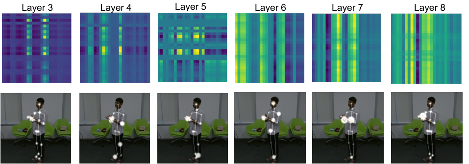
In Figure 6, we report some actions and the corresponding Spatial Self-Attention maps. On the top we draw the skeleton of the subjects, where the radius of the circles in correspondence to each joint is proportional its relevance predicted by the self-attention. The heatmaps on the bottom represent the attention scores of the last layer; these are matrices, where each row and each column represents a body joint. An element in position represents the predicted correlation between joint and joint in the same frame. As it can be observed, depending on the action, different parts of the body are activated. In Figure 7 are shown the same heatmaps at each layer. In the first layers, self-attention captures low-level correlations between body joints, as highlighted by the sparsity of the activations. While going deeper through the network, the global importance of each node emerges instead, as highlighted by the vertical lines corresponding to the most relevant joints.
8 Conclusions
In this paper we propose a novel approach that introduces Transformer self-attention in skeleton activity recognition as an alternative to graph convolution. Through extensive experiments on NTU-60, NTU-120 and Kinetics, we demonstrated that our Spatial Self-Attention module (SSA) can replace graph convolution, enabling more flexible and dynamic representations. Similarly, Temporal Self-Attention module (TSA) overcomes the strict locality of standard convolution, enabling the extraction of long-range dependencies across the action. Moreover, our final Spatial-Temporal Transformer network (ST-TR) achieves state-of-the-art performance on all dataset w.r.t. methods using same input joint information and stream setup, and results on-par with state-of-the-art methods when bones information is added. As configurations only involving self-attention modules revealed to be sub-optimal, a possible future work is to search for a unified Transformer architecture able to replace graph convolution in a variety of tasks.

References
- Aggarwal and Ryoo (2011) Aggarwal, J.K., Ryoo, M.S., 2011. Human activity analysis: A review. ACM Computing Surveys (CSUR) 43, 1–43.
- Bello et al. (2019a) Bello, I., Zoph, B., Vaswani, A., Shlens, J., Le, Q.V., 2019a. Attention augmented convolutional networks, in: Proceedings of the IEEE/CVF International Conference on Computer Vision (ICCV).
- Bello et al. (2019b) Bello, I., Zoph, B., Vaswani, A., Shlens, J., Le, Q.V., 2019b. Attention augmented convolutional networks. Proceedings of the IEEE International Conference on Computer Vision , 3286–3295.
- Bronstein et al. (2017) Bronstein, M.M., Bruna, J., LeCun, Y., Szlam, A., Vandergheynst, P., 2017. Geometric deep learning: going beyond euclidean data. IEEE Signal Processing Magazine 34, 18–42.
- Bruna et al. (2014) Bruna, J., Zaremba, W., Szlam, A., Lecun, Y., 2014. Spectral networks and locally connected networks on graphs. International Conference on Learning Representations (ICLR2014), CBLS, April 2014 .
- Cao et al. (2019) Cao, Z., Hidalgo Martinez, G., Simon, T., Wei, S., Sheikh, Y.A., 2019. Openpose: Realtime multi-person 2d pose estimation using part affinity fields. IEEE Transactions on Pattern Analysis and Machine Intelligence .
- Carion et al. (2020) Carion, N., Massa, F., Synnaeve, G., Usunier, N., Kirillov, A., Zagoruyko, S., 2020. End-to-end object detection with transformers, in: European Conference on Computer Vision, Springer. pp. 213–229.
- Cheng et al. (2020) Cheng, K., Zhang, Y., He, X., Chen, W., Cheng, J., Lu, H., 2020. Skeleton-based action recognition with shift graph convolutional network. Proceedings of the IEEE/CVF Conference on Computer Vision and Pattern Recognition , 183–192.
- Chéron et al. (2015) Chéron, G., Laptev, I., Schmid, C., 2015. P-cnn: Pose-based cnn features for action recognition. Proceedings of the IEEE international conference on computer vision , 3218–3226.
- Cho et al. (2020) Cho, S., Maqbool, M., Liu, F., Foroosh, H., 2020. Self-attention network for skeleton-based human action recognition, in: Proceedings of the IEEE/CVF Winter Conference on Applications of Computer Vision, pp. 635–644.
- Defferrard et al. (2016) Defferrard, M., Bresson, X., Vandergheynst, P., 2016. Convolutional neural networks on graphs with fast localized spectral filtering. Advances in neural information processing systems , 3844–3852.
- Ding et al. (2017) Ding, Z., Wang, P., Ogunbona, P.O., Li, W., 2017. Investigation of different skeleton features for cnn-based 3d action recognition. 2017 IEEE International Conference on Multimedia & Expo Workshops (ICMEW) , 617–622.
- Dosovitskiy et al. (2020) Dosovitskiy, A., Beyer, L., Kolesnikov, A., Weissenborn, D., Zhai, X., Unterthiner, T., Dehghani, M., Minderer, M., Heigold, G., Gelly, S., et al., 2020. An image is worth 16x16 words: Transformers for image recognition at scale. arXiv preprint arXiv:2010.11929 .
- Du et al. (2015) Du, Y., Wang, W., Wang, L., 2015. Hierarchical recurrent neural network for skeleton based action recognition. Proceedings of the IEEE conference on computer vision and pattern recognition , 1110–1118.
- Gori et al. (2005) Gori, M., Monfardini, G., Scarselli, F., 2005. A new model for learning in graph domains. Proceedings. 2005 IEEE International Joint Conference on Neural Networks, 2005. 2, 729–734.
- He et al. (2020) He, S., Liao, W., Tavakoli, H.R., Yang, M., Rosenhahn, B., Pugeault, N., 2020. Image captioning through image transformer, in: Proceedings of the Asian Conference on Computer Vision.
- Henaff et al. (2015) Henaff, M., Bruna, J., LeCun, Y., 2015. Deep convolutional networks on graph-structured data. arXiv preprint arXiv:1506.05163 .
- Hu et al. (2015) Hu, J.F., Zheng, W.S., Lai, J., Zhang, J., 2015. Jointly learning heterogeneous features for rgb-d activity recognition. Proceedings of the IEEE conference on computer vision and pattern recognition , 5344–5352.
- Huang et al. (2019) Huang, Z., Wang, X., Huang, L., Huang, C., Wei, Y., Liu, W., 2019. Ccnet: Criss-cross attention for semantic segmentation, in: Proceedings of the IEEE/CVF International Conference on Computer Vision, pp. 603–612.
- Hussein et al. (2013) Hussein, M.E., Torki, M., Gowayyed, M.A., El-Saban, M., 2013. Human action recognition using a temporal hierarchy of covariance descriptors on 3d joint locations. Twenty-third international joint conference on artificial intelligence .
- Ioffe and Szegedy (2015) Ioffe, S., Szegedy, C., 2015. Batch normalization: Accelerating deep network training by reducing internal covariate shift. arXiv preprint arXiv:1502.03167 .
- Kay et al. (2017) Kay, W., Carreira, J., Simonyan, K., Zhang, B., Hillier, C., Vijayanarasimhan, S., Viola, F., Green, T., Back, T., Natsev, P., et al., 2017. The kinetics human action video dataset. arXiv preprint arXiv:1705.06950 .
- Ke et al. (2018) Ke, Q., Bennamoun, M., An, S., Sohel, F., Boussaid, F., 2018. Learning clip representations for skeleton-based 3d action recognition. IEEE Transactions on Image Processing 27, 2842–2855.
- Keselman et al. (2017) Keselman, L., Iselin Woodfill, J., Grunnet-Jepsen, A., Bhowmik, A., 2017. Intel realsense stereoscopic depth cameras, in: Proceedings of the IEEE Conference on Computer Vision and Pattern Recognition Workshops, pp. 1–10.
- Kipf and Welling (2017) Kipf, T.N., Welling, M., 2017. Semi-supervised classification with graph convolutional networks. 5th International Conference on Learning Representations, ICLR .
- Lee et al. (2020) Lee, S., Yu, Y., Kim, G., Breuel, T., Kautz, J., Song, Y., 2020. Parameter efficient multimodal transformers for video representation learning. arXiv preprint arXiv:2012.04124 .
- Lev et al. (2016) Lev, G., Sadeh, G., Klein, B., Wolf, L., 2016. Rnn fisher vectors for action recognition and image annotation. European Conference on Computer Vision , 833–850.
- Li et al. (2017) Li, B., Dai, Y., Cheng, X., Chen, H., Lin, Y., He, M., 2017. Skeleton based action recognition using translation-scale invariant image mapping and multi-scale deep cnn. ICMEW .
- Li et al. (2019) Li, M., Chen, S., Chen, X., Zhang, Y., Wang, Y., Tian, Q., 2019. Actional-structural graph convolutional networks for skeleton-based action recognition, in: Proceedings of the IEEE/CVF Conference on Computer Vision and Pattern Recognition, pp. 3595–3603.
- Liu et al. (2019) Liu, J., Shahroudy, A., Perez, M.L., Wang, G., Duan, L.Y., Chichung, A.K., 2019. Ntu rgb+d 120: A large-scale benchmark for 3d human activity understanding. IEEE transactions on pattern analysis and machine intelligence .
- Liu et al. (2016) Liu, J., Shahroudy, A., Xu, D., Wang, G., 2016. Spatio-temporal lstm with trust gates for 3d human action recognition. European conference on computer vision , 816–833.
- Liu et al. (2017a) Liu, J., Wang, G., Duan, L.Y., Abdiyeva, K., Kot, A.C., 2017a. Skeleton-based human action recognition with global context-aware attention lstm networks. IEEE Transactions on Image Processing 27, 1586–1599.
- Liu et al. (2017b) Liu, J., Wang, G., Hu, P., Duan, L.Y., Kot, A.C., 2017b. Global context-aware attention lstm networks for 3d action recognition. Proceedings of the IEEE Conference on Computer Vision and Pattern Recognition , 1647–1656.
- Liu et al. (2017c) Liu, M., Liu, H., Chen, C., 2017c. Enhanced skeleton visualization for view invariant human action recognition. Pattern Recognition 68, 346–362.
- Liu and Yuan (2018) Liu, M., Yuan, J., 2018. Recognizing human actions as the evolution of pose estimation maps. Proceedings of the IEEE Conference on Computer Vision and Pattern Recognition , 1159–1168.
- Liu et al. (2020) Liu, Z., Zhang, H., Chen, Z., Wang, Z., Ouyang, W., 2020. Disentangling and unifying graph convolutions for skeleton-based action recognition. Proceedings of the IEEE/CVF Conference on Computer Vision and Pattern Recognition , 143–152.
- Micheli (2009) Micheli, A., 2009. Neural network for graphs: A contextual constructive approach. IEEE Transactions on Neural Networks 20, 498–511.
- Nguyen and Salazar (2019) Nguyen, T.Q., Salazar, J., 2019. Transformers without tears: Improving the normalization of self-attention. arXiv preprint arXiv:1910.05895 .
- Niepert et al. (2016) Niepert, M., Ahmed, M., Kutzkov, K., 2016. Learning convolutional neural networks for graphs. International conference on machine learning , 2014–2023.
- Oord et al. (2016) Oord, A.v.d., Kalchbrenner, N., Vinyals, O., Espeholt, L., Graves, A., Kavukcuoglu, K., 2016. Conditional image generation with pixelcnn decoders. arXiv preprint arXiv:1606.05328 .
- Parmar et al. (2018) Parmar, N., Vaswani, A., Uszkoreit, J., Kaiser, L., Shazeer, N., Ku, A., Tran, D., 2018. Image transformer, in: International Conference on Machine Learning, PMLR. pp. 4055–4064.
- Paszke et al. (2019) Paszke, A., Gross, S., Massa, F., Lerer, A., Bradbury, J., Chanan, G., Killeen, T., Lin, Z., Gimelshein, N., Antiga, L., et al., 2019. Pytorch: An imperative style, high-performance deep learning library, pp. 8026–8037.
- Ren et al. (2020) Ren, B., Liu, M., Ding, R., Liu, H., 2020. A survey on 3d skeleton-based action recognition using learning method. arXiv preprint arXiv:2002.05907 .
- Scarselli et al. (2008) Scarselli, F., Gori, M., Tsoi, A.C., Hagenbuchner, M., Monfardini, G., 2008. The graph neural network model. IEEE Transactions on Neural Networks 20, 61–80.
- Shahroudy et al. (2016) Shahroudy, A., Liu, J., Ng, T.T., Wang, G., 2016. Ntu rgb+d: A large scale dataset for 3d human activity analysis. Proceedings of the IEEE conference on computer vision and pattern recognition , 1010–1019.
- Shi et al. (2019a) Shi, L., Zhang, Y., Cheng, J., Lu, H., 2019a. Skeleton-based action recognition with directed graph neural networks. Proceedings of the IEEE Conference on Computer Vision and Pattern Recognition , 7912–7921.
- Shi et al. (2019b) Shi, L., Zhang, Y., Cheng, J., Lu, H., 2019b. Two-stream adaptive graph convolutional networks for skeleton-based action recognition. Proceedings of the IEEE Conference on Computer Vision and Pattern Recognition , 12026–12035.
- Si et al. (2019) Si, C., Chen, W., Wang, W., Wang, L., Tan, T., 2019. An attention enhanced graph convolutional lstm network for skeleton-based action recognition. Proceedings of the IEEE conference on computer vision and pattern recognition , 1227–1236.
- Simonyan and Zisserman (2014) Simonyan, K., Zisserman, A., 2014. Two-stream convolutional networks for action recognition in videos. Advances in neural information processing systems , 568–576.
- Song et al. (2017) Song, S., Lan, C., Xing, J., Zeng, W., Liu, J., 2017. An end-to-end spatio-temporal attention model for human action recognition from skeleton data. Proceedings of the Thirty-First AAAI Conference on Artificial Intelligence , 4263–4270.
- Such et al. (2017) Such, F.P., Sah, S., Domínguez, M., Pillai, S., Zhang, C., Michael, A., Cahill, N.D., Ptucha, R.W., 2017. Robust spatial filtering with graph convolutional neural networks. IEEE Journal of Selected Topics in Signal Processing .
- Vaswani et al. (2017) Vaswani, A., Shazeer, N., Parmar, N., Uszkoreit, J., Jones, L., Gomez, A.N., Kaiser, Ł., Polosukhin, I., 2017. Attention is all you need. Advances in neural information processing systems , 5998–6008.
- Vemulapalli et al. (2014) Vemulapalli, R., Arrate, F., Chellappa, R., 2014. Human action recognition by representing 3d skeletons as points in a lie group. Proceedings of the IEEE conference on computer vision and pattern recognition , 588–595.
- Wang and Wang (2017) Wang, H., Wang, L., 2017. Modeling temporal dynamics and spatial configurations of actions using two-stream recurrent neural networks. Proceedings of the IEEE Conference on Computer Vision and Pattern Recognition , 499–508.
- Wang et al. (2019) Wang, L., Huynh, D.Q., Koniusz, P., 2019. A comparative review of recent kinect-based action recognition algorithms. IEEE Transactions on Image Processing 29, 15–28.
- Wang et al. (2018) Wang, X., Girshick, R., Gupta, A., He, K., 2018. Non-local neural networks, in: 2018 IEEE/CVF Conference on Computer Vision and Pattern Recognition, pp. 7794–7803. doi:10.1109/CVPR.2018.00813.
- Yan et al. (2018) Yan, S., Xiong, Y., Lin, D., 2018. Spatial temporal graph convolutional networks for skeleton-based action recognition. Thirty-second AAAI conference on artificial intelligence .
- Zehui et al. (2019) Zehui, L., Liu, P., Huang, L., Fu, J., Chen, J., Qiu, X., Huang, X., 2019. Dropattention: A regularization method for fully-connected self-attention networks. arXiv preprint arXiv:1907.11065 .
- Zhang et al. (2019) Zhang, H.B., Zhang, Y.X., Zhong, B., Lei, Q., Yang, L., Du, J.X., Chen, D.S., 2019. A comprehensive survey of vision-based human action recognition methods. Sensors 19, 1005.
- Zhang et al. (2017) Zhang, P., Lan, C., Xing, J., Zeng, W., Xue, J., Zheng, N., 2017. View adaptive recurrent neural networks for high performance human action recognition from skeleton data. Proceedings of the IEEE International Conference on Computer Vision , 2117–2126.
- Zhang (2012) Zhang, Z., 2012. Microsoft kinect sensor and its effect. IEEE multimedia 19, 4–10.
- Zhao et al. (2020) Zhao, H., Jiang, L., Jia, J., Torr, P., Koltun, V., 2020. Point transformer. arXiv preprint arXiv:2012.09164 .