Model-Reference Reinforcement Learning for Collision-Free Tracking Control of Autonomous Surface Vehicles

Let $\bm{x}=\left[\bm{\eta}^{T},\bm{\nu}^{T}\right]^{T}$ and $\bm{u}=\bm{\tau}$, so (1) can be rewritten as

where $\bm{A}\left(\bm{\nu}\right)=\bm{M}^{-1}\left(\bm{C}\left(\bm{\nu}\right)+\bm{D}\left(\bm{\nu}\right)\right)$, and $\bm{B}=\bm{M}^{-1}$. Assuming that an accurate model (5) is not available, it is possible to get a nominal model expressed as

where $\bm{A}_{m}$ and $\bm{B}_{m}$ are the known system matrices, and the unmodelled dynamics $\bm{G}\left(\bm{\nu}\right)$ ignored. Note that $\bm{A}_{m}$ and $\bm{B}_{m}$ are different from $\bm{A}\left(\bm{\nu}\right)$ and $\bm{B}$, respectively. In $\bm{A}_{m}$ and $\bm{B}_{m}$, we will ignore all unknown nonlinear terms, and obtain a linear nominal model. Assume that there exists a control law $\bm{u}_{m}$ allowing the states of the nominal system (6) to converge to a reference signal $\bm{x}_{r}$, i.e., $\|\bm{x}_{m}-\bm{x}_{r}\|_{2}\to{0}$ as $t\to\infty$.

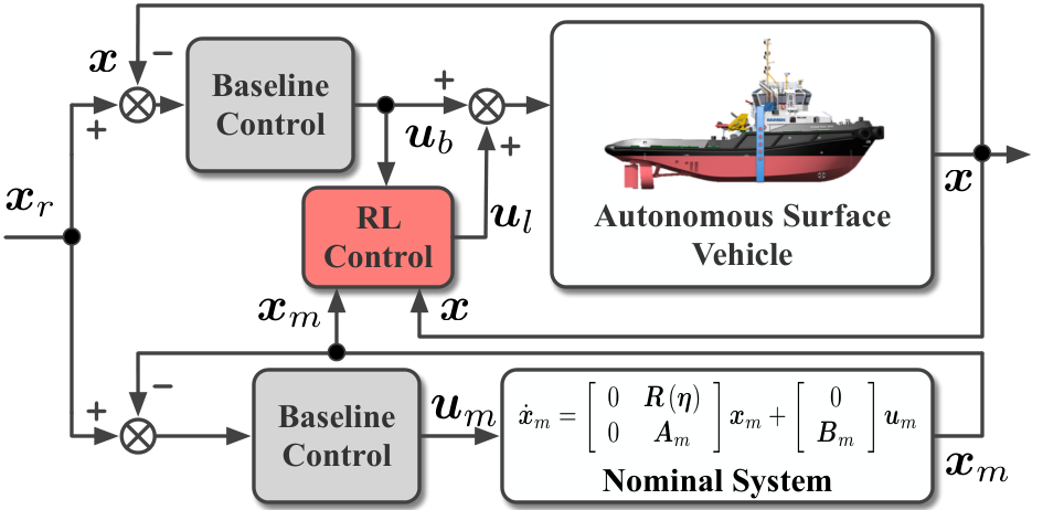
The objective of the work in this paper is to design a controller allowing the state $\bm{x}$ to track state trajectories of the nominal model (6) and avoid collisions with obstacles having known states $\bm{x}_{{o}_{i}}$, where $i\in\left\{1,\ldots,N_{o}\right\}$ indicates the $i$-th obstacle. As shown in Figure 2, the overall control structure for the ASV system (5) is

where $\bm{u}_{b}$ is a baseline control designed based on (6), and $\bm{u}_{l}$ is a control law from the deep RL module whose design is provided in Section IV-B.

For the formulation of RL, the ASV dynamics (5) and (6) are characterized using another mathematical model called Markov decision process that is denoted by a tuple $\mathcal{MDP}:=\big\langle\mathcal{S},\;\mathcal{U},\;\mathcal{P},\;R,\;\gamma\big\rangle$, where $\mathcal{S}$ is the state space, $\mathcal{U}$ specifies the action/input space, $\mathcal{P}:\mathcal{S}\times\mathcal{U}\times\mathcal{S}\rightarrow\mathbb{R}$ defines a transition probability, $R:\mathcal{S}\times\mathcal{U}\rightarrow\mathbb{R}$ is a reward function, and $\gamma\in\left[0,\;1\right)$ is a discount factor. Note that the state vector $\bm{s}\in\mathcal{S}$ contains all available signals affecting the learned control $\bm{u}_{l}$. In this paper, such signals include $\bm{x}$, $\bm{x}_{m}$, $\bm{x}_{r}$, $\bm{u}_{b}$, and $\bm{x}_{{o}_{i}}$, where $\bm{x}_{m}$ represents the desired behaviour of the system (5) and $\bm{u}_{b}$ is a function of $\bm{x}$ and $\bm{x}_{r}$, and $\bm{x}_{{o}_{i}}$ are obstacle states in the neighbourhood (e.g., the position and velocity of the $i$-th obstacle). Hence, $\bm{s}=\left\{\bm{x}_{m},\bm{x},\bm{u}_{b},\cup_{i}^{N_{o}}\bm{x}_{{o}_{i}}\right\}$, where $\cup_{i}^{N_{o}}\bm{x}_{{o}_{i}}$ denotes the states of $N_{o}$ obstacles detected by the ASV. More details on obstacles will be discussed in Section III-D.

Since RL learns the control policies using data samples, it is assumed that we can sample input and state data from system (5) at discrete time steps. The sample time step is fixed and denoted by $\delta t$. Without loss of generality, let $\bm{x}_{t}$, $\bm{u}_{b,t}$, and $\bm{u}_{l,t}$ be the ASV state, the baseline control action, and the control action from RL at the time step $t$, respectively. The union of obstacles detected by the ASV is characterized by $\cup_{i}^{N_{o}}\bm{x}_{{o}_{i},t}$. The state signal $\bm{s}$ at the time step $t$ is, therefore, denoted by $\bm{s}_{t}=\left\{\bm{x}_{m,t},\bm{x}_{t},\bm{u}_{b,t},\cup_{i}^{N_{o}}\bm{x}_{{o}_{i},t}\right\}$.

For standard RL, the objective is to maximize an expected accumulated return described by a value function $V_{\bm{\pi}}\left(\bm{s}_{t}\right)$ with

where $\mathcal{P}_{t+1|t}=\mathcal{P}\left(\bm{s}_{t+1}\left|\bm{s}_{t},\bm{u}_{l,t}\right.\right)$ is the transition probability of the ASV system, $R_{t}=R(\bm{s}_{t},\bm{u}_{l,t})$ is the reward function, $\gamma\in\left[0,1\right)$ is a constant discount factor, and $\bm{\pi}\left(\bm{u}_{l,t}|\bm{s}_{t}\right)$ is called control policy in RL. A policy in RL, denoted by $\bm{\pi}\left(\bm{u}_{l,t}|\bm{s}_{t}\right)$, is the probability of choosing an action $\bm{u}_{l,t}\in\mathcal{U}$ at a state $\bm{s}_{t}\in\mathcal{S}$ [27]. In this paper, a Gaussian policy is used, which is

where $\mathcal{N}\left(\cdot,\cdot\right)$ denotes a Gaussian distribution with ${\bm{u}}_{l}\left(\bm{s}\right)$ as the mean value and $\bm{\sigma}$ as the covariance matrix. The covariance matrix $\bm{\sigma}$ controls the exploration performance at the learning stage. For the algorithm design, we also introduce an action-value function (a.k.a., Q-function) defined by

where $\mathbb{E}_{\bm{s}_{t+1}}\left[\cdot\right]=\sum_{\bm{s}_{t+1}}\mathcal{P}_{t+1|t}\left[\cdot\right]$ is an expectation operator over the distribution of $\bm{s}_{t+1}$. Maximizing $Q_{\bm{\pi}}\left(\bm{s}_{t},\;\bm{u}_{l,t}\right)$ is equivalent to maximizing $V_{\bm{\pi}}(\bm{s}_{t})$. In the sequel, we will focus the maximization of $Q_{\bm{\pi}}\left(\bm{s}_{t},\bm{u}_{l,t}\right)$ instead of $V_{\bm{\pi}}(s_{t})$.

In this paper, the deep RL is resolved based on the soft actor-critic (SAC) algorithm which provides both sample efficient learning and convergence [50]. In SAC, an entropy term is added to regulate the exploration performance at the training stage, thus resulting in a modified Q-function in (11).

where $\mathcal{H}\left(\bm{\pi}\left(\bm{u}_{l,t}|\bm{s}_{t}\right)\right)=-\sum_{\bm{u}_{l,t}}\bm{\pi}\left(\bm{u}_{l,t}|\bm{s}_{t}\right)\ln\left(\bm{\pi}\left(\bm{u}_{l,t}|\bm{s}_{t}\right)\right)=-\mathbb{E}_{\bm{\pi}}\left[\ln\left(\bm{\pi}\left(\bm{u}_{l,t}|\bm{s}_{t}\right)\right)\right]$ is the entropy of the policy, and $\alpha$ is a temperature parameter [50]. Hence, SAC aims to solve the following optimization problem.

where $\Pi$ denotes a policy set.

Training/learning process of SAC will repeatedly execute policy evaluation and policy improvement. In the policy evaluation, the Q-value in (11) is computed by applying a Bellman operation $Q_{\bm{\pi}}\left(\bm{s}_{t},\bm{u}_{l,t}\right)=\mathcal{T}^{\bm{\pi}}Q_{\bm{\pi}}\left(\bm{s}_{t},\bm{u}_{l,t}\right)$ where

In the policy improvement, the policy is updated by

where $\bm{\pi}_{old}$ denotes the policy from the last update, $Q^{{\bm{\pi}}_{old}}$ is the Q-value of $\bm{\pi}_{old}$, $\mathscr{D}_{KL}$ denotes the Kullback-Leibler (KL) divergence, and $Z^{{\pi}_{old}}$ is a normalization factor. Via mathematical manipulations, the objective is transformed into

More details on how (15) is obtained can be found in [50].

In our design, two objectives are defined for the ASV: trajectory tracking and collision avoidance. For the trajectory tracking, we aim to allow system (5) to track the nominal system (6), so the tracking reward $R_{t,1}$ is defined as

where $\bm{H}_{1}>0$ and $\bm{H}_{2}>0$ are positive definite matrices.

The second objective is to avoid obstacles along the trajectory of the ASV. Figure 3 shows variables used for the definition of the reward function for collision avoidance. All obstacles are assumed to be inscribed in a circle. The maximum size of the $i$-th obstacle is defined by $d_{{o}_{i}}$ as shown in Figure 3. The size of the ASV is denoted by $d_{a}$. We introduce a safe region with a radius of $d_{{s}_{i}}$ for the $i$-th agent, where $d_{{s}_{i}}>d_{{o}_{i}}+d_{a}$. The relative distance between the $i$-th obstacle and the ASV is defined as $d_{a{o}_{i}}$. If $d_{a{o}_{i}}\leq d_{d}$, the $i$-th obstacle is visible to the ASV, where $d_{d}$ is the radius of the detection region of the ASV. Note that the obstacles could be either static or moving, so the state vector the $i$-th obstacle is written as $\bm{x}_{{o}_{i}}=\left[\bm{p}_{{o}_{i}}^{T},\bm{v}_{{o}_{i}}^{T}\right]^{T}$, where $\bm{p}_{{o}_{i}}$ is the position of the $i$-th obstacle, and $\bm{v}_{{o}_{i}}$ is the velocity of the $i$-th obstacle. Let $\bm{p}_{a}=\left[x_{p},y_{p}\right]^{T}$ and $\bm{v}_{a}=\left[u_{p},v_{p}\right]^{T}$ be the position and velocity of the ASV, respectively. For the $i$-th visible obstacle at the time step $t$, define the following variable shown in Figure 4.

where “^×” denotes the cross product operation, $d_{i,t}$ represents the closest possible distance between the ASV and the obstacle, if the ASV keeps its current moving direction relative to the obstacle. Note that $d_{i,t}$ is only meaningful, if $\left(\bm{v}_{a}-\bm{v}_{{o}_{i}}\right)^{T}\left(\bm{p}_{{o}_{i}}-\bm{p}_{a}\right)>0$. If $\left(\bm{v}_{a}-\bm{v}_{{o}_{i}}\right)^{T}\left(\bm{p}_{{o}_{i}}-\bm{p}_{a}\right)>0$, it implies that the ASV moves towards the obstacle, otherwise, the ASV moves away from the obstacle. Therefore, the reward function for collision avoidance is defined to be

where $q_{c,i}>0$ is the maximum possible cost for collisions, $c_{i}>0$ is a design parameter, and $\mathbbm{1}_{{o}_{i}}\left(\bm{x}_{{o}_{i}},\bm{p}_{a},\bm{v}_{a}\right)$ is

The parameter $c_{i}>0$ adjusts the sensitivity of collision avoidance of RL in related to the $i$-th obstacle. The influence of $c_{i}>0$ on $R_{t,2}$ is illustrated in Figure 5.

The overall reward function is, therefore, defined to be

In RL, the value function $Q_{\bm{\pi}}\left(\bm{s}_{t},\bm{u}_{l,t}\right)$, which contains future information as shown in (10), is not known in advance. Similarly, the control policy $\bm{\pi}$ is unknown as well. Hence, a feasible solution is to approximate both the value function $Q_{\bm{\pi}}\left(\bm{s}_{t},\bm{u}_{l,t}\right)$ and the control policy $\bm{\pi}$ using deep neural networks. In this paper, the deep neural networks used to approximate both the value function $Q_{\bm{\pi}}\left(\bm{s}_{t},\bm{u}_{l,t}\right)$ and the policy $\bm{\pi}\left(\bm{u}_{l,t}|\bm{s}_{t}\right)$ are chosen to be fully connected multiple layer perceptrons (MLP) with rectified linear unit (ReLU) nonlinearities as the activation functions. The ReLU nonlinearities are defined by

The ReLU activation function outperforms other activation functions like sigmoid functions [51]. For a vector $z=[z_{1}\text{, }\ldots,\text{, }z_{n}]^{T}\in\mathbb{R}^{n}$, there exists $\underline{relu}\left(z\right)=[\underline{relu}\left(z_{1}\right)\text{, }\ldots\text{, }\underline{relu}\left(z_{n}\right)]^{T}$. As an example, a MLP with “ReLU” as the activation functions and two hidden layers is

where $\left[z^{T}\text{, }1\right]^{T}$ is a vector composed of $z$ and a bias $1$, the superscript “$2$” denotes the total number of hidden layers, the subscript “$\mathrm{w}$” denotes the parameter set to be trained in a MLP with $\mathrm{w}=\left\{\mathrm{w}_{0}\text{, }\mathrm{w}_{1}\text{, }\mathrm{w}_{2}\right\}$, and $\mathrm{w}_{0}$, $\mathrm{w}_{1}$, and $\mathrm{w}_{2}$ are weight matrices with appropriate dimensions.

If there is a set of inputs $z=\left\{z_{1}\text{, }\ldots\text{, }z_{L}\right\}$ for the MLP in (20) with $z_{1}$, $\ldots$, $z_{L}$ denoting vector signals, we have

Besides, $\underline{MLP}_{\mathrm{w}}^{2}\left(z_{1}\text{, }z_{2}\right)=\underline{MLP}_{\mathrm{w}}^{2}\left(\left[z_{1}^{T}\text{, }z_{2}^{T}\right]^{T}\right)$ for two vector inputs $z_{1}$ and $z_{2}$. If $z_{1}=\left\{z_{11}\text{, }\ldots\text{, }z_{1L}\right\}$ is a set of vectors, $\underline{MLP}_{\mathrm{w}}^{2}\left(z_{1}\text{, }z_{2}\right)=\underline{MLP}_{\mathrm{w}}^{2}\left(\left[z_{11}^{T}\text{, }\ldots\text{, }z_{1L}^{T},z_{2}^{T}\right]^{T}\right)$.

Let $Q_{\theta}\left(\bm{s}_{t},\bm{u}_{l,t}\right)$ be the approximated Q-function using a MLP with a set of parameters denoted by $\theta$. Following (20) and (21), the Q-function approximation $Q_{\theta}\left(\bm{s}_{t},\bm{u}_{l,t}\right)$ is

where $\theta=\left\{\theta_{0},\ldots,\theta_{{K}_{1}}\right\}$ with $\theta_{i}\in\mathbb{R}^{{\left(L\right)}\times{\left(L+1\right)}}$ for $0\leq i\leq K_{1}$ denoting the weight matrices with proper dimensions. The deep neural network for $Q_{\theta}$ is illustrated in Figure 6.

The control law $\bm{u}_{l}$ is also approximated using a MLP. The approximated control law of $\bm{u}_{l}$ with a parameter set $\phi$ is

The illustration of ${\bm{u}}_{l,\phi}$ is given in Figure 6. In SAC, there are two outputs for the MLP in (23). One is the control law ${\bm{u}}_{l,\phi}$, the other one is ${\sigma}_{\phi}$ that is the standard deviation of the exploration noise [50]. According to (9), the parameterized policy $\bm{\pi}_{{\phi}}$ in our model-reference RL is

The deep neural network for $Q_{\theta}$ is called critic, while the one for $\bm{\pi}_{{\phi}}$ is called actor.

The algorithm training process is illustrated in Figure 7. The whole training process will be offline. We repeatedly run the system (5) under a trajectory tracking task. At each time step $t+1$, we collect data samples, such as an input from the last time step $\bm{u}_{l,t}$, a state from the last time step $\bm{s}_{t}$, a reward $R_{t}$, and a current state $\bm{s}_{t+1}$. Those historical data will be stored as a tuple $\left(\bm{s}_{t},\bm{u}_{l,t},R_{t},\bm{s}_{t+1}\right)$ at a replay memory $\mathcal{D}$ [52]. At each policy evaluation or improvement step, we randomly sample a batch of historical data, $\mathcal{B}$, from the replay memory $\mathcal{D}$ for the training of the parameters $\theta$ and $\phi$. Starting the training, we apply the baseline control policy $\bm{u}_{b}$ to an ASV system to collect the initial data $\mathcal{D}_{0}$ as shown in Algorithm 1. The initial data set $\mathcal{D}_{0}$ is used for the initial fitting of Q-value functions. When the initialization is over, we execute both $\bm{u}_{b}$ and the latest updated RL policy $\bm{\pi}_{{\phi}}\left(\bm{u}_{l,t}|\bm{s}_{t}\right)$ to run the ASV system.

At the policy evaluation step, the parameters $\theta$ are trained to minimize the following Bellman residual.

where $\left(\bm{s}_{t},\bm{u}_{l,t}\right)\sim\mathcal{D}$ implies that we randomly pick data samples $\left(\bm{s}_{t},\bm{u}_{l,t}\right)$ from a replay memory $\mathcal{D}$, and

where $\bar{\theta}$ is the target parameter which will be updated slowly. Applying a stochastic gradient descent technique (ADAM [53] in this paper) to (25) on a data batch $\mathcal{B}$ with a fixed size yields

where $|\mathcal{B}|$ is the batch size.

At the policy improvement step, the objective function defined in (15) is represented using data samples from the replay memory $\mathcal{D}$ as given in (26).

Parameter $\phi$ is trained to minimize (26) using a stochastic gradient descent technique. Applying the policy gradient technique to (26), we can calculate the gradient of $J_{\bm{\pi}}\left(\phi\right)$ with respect to $\phi$ in terms of the stochastic gradient method as

The temperature parameters $\alpha$ are updated by minimizing

where $\bar{\mathcal{H}}$ is a target entropy. In the final implementation, two critics are introduced to reduce the over-estimation issue in the training of critic neural networks [54]. Under the two-critic mechanism, the target value $Y_{target}$ is modified to be

The entire process is summarized in Algorithm 1, in which $\iota_{Q}$, $\iota_{\pi}$, $\iota_{\alpha}>0$ are learning rates, and $\kappa>0$ is a constant scalar.

Once the training process is over, Algorithm 1 will output the optimal parameters for the deep neural networks in (22) and (23). Once the optimal parameters are obtained, the learned control law $\bm{u}_{l}$ is approximated by

where $\phi^{*}$ is the optimal parameter set for the MLP in (23) and is obtained via Algorithm 1.

The general structure of a deep RL algorithm is summarized in Algorithm 2. The learning process will recursively execute the policy evaluation and policy improvement until convergence. As we mentioned in Section III-A, the baseline control $\bm{u}_{b}$ is assumed to stabilize the ASV without collision avoidance. Therefore, the following assumption is introduced for the convergence analysis.

According to (16) and (18), both $R_{t,1}$ and $R_{t,2}$ are non-positive. With Assumption 1, the reward function $R_{t,1}$ is ensured to be bounded. Additionally, the reward function $R_{t,2}$ is bounded by design as shown in Figure 5 for a finite number of obstacles. Hence, the overall reward $R_{t}$ is bounded, namely

where $R_{min}$ is the lowest bound for the reward function under the baseline control $\bm{u}_{b}$.

In terms of (30), we can present the following Lemma 1 and Lemma 2 for the convergence analysis of the entropy-regularized SAC algorithm [50, 55].

In terms of (1) and (2), we are ready to present Theorem 1 to show the convergence of the model-reference RL algorithm. In the sequel, the superscript $i$ denotes the $i$-th iteration of the policy iteration algorithm or the $i$-th policy improvement, where $i=0$, $1$, $\ldots$, $\infty$.

In this subsection, we will show the closed-loop stability of the overall control law (baseline control $\bm{u}_{b}$ plus the learned control $\bm{u}_{l}$) for the tracking control without obstacles. The closed-loop stability is analyzed under the general tracking performance without the consideration of collision avoidance, as the tracking control is the fundamental task. Before the closed-loop stability is analyzed, the admissible control concept is introduced in Definition 1, which is similar to the admissible control in adaptive dynamic programming [56, 57, 58].

Note that the admissible control in [56, 57, 58] needs to provide the asymptotic stability for the system. However, the admissible control in Definition 1 doesn’t necessarily ensure the system (5) to be asymptotically stable. Hence, the admissible control concept in this paper is less conservative than that in [56, 57, 58].

Assume that the baseline control $\bm{u}_{b}$ developed using the nominal system (6) of the ASV (5) is an admissible control law for the uncertain system (5). Let $\Delta\left(t\right)$ be the overall uncertainties in (5). Without loss of generality, it is assumed that $\Delta\left(t\right)$ is bounded, namely $\|\Delta\left(t\right)\|_{\mathcal{L}_{\infty}}\leq\bar{\Delta}$ where $\|\cdot\|_{\mathcal{L}_{\infty}}$ denotes the $\mathcal{L}_{\infty}$ norm. In this paper, the objective of the tracking control in obstacle-free environment is to ensure that the ASV system (5) can track its desired behaviour defined by its nominal system (6), namely $\|\bm{x}-\bm{x}_{m}\|_{2}\to{0}$ as $t\to\infty$. Let $\bm{e}_{t}=\bm{x}_{t}-\bm{x}_{m,t}$ be the tracking error of the ASV at the time instant $t$. The following assumption is made for a admissible baseline control $\bm{u}_{b}$ according to Definition 1 and Theorem 4.18 in [59] (Chapter 4, Page 172).

Assumption 2 is possible in real world. One can treat the nominal model (6) as a linearized model of the overall ASV system (5) around a certain equilibrium. Assumption 2 presents the basic design requirements for the baseline control law. With a baseline control law satisfying Assumption $1$, we could obtain two advantages which makes the RL process more efficient. Firstly, it can ensure that the reward function $R_{t}$ is bounded, implying that both $V_{\bm{\pi}}(\bm{s}_{t+1})$ and $Q\left(\bm{s}_{t},\bm{u}_{l,t}\right)$ are bounded. Secondly, it could provide a “warm” start for the RL process.

With a feasible baseline control, the uncertain ASV system can be ensured to be stable during the entire learning process. In the stability analysis, we ignore the entropy term $\mathcal{H}\left(\bm{\pi}\right)$, as it will converge to zero in the end and it is only introduced to regulate the exploration magnitude. Hence, exploration noises will be set to be zero. Now, we present Theorem 2 to demonstrate the closed-loop stability of the ASV system (5) under the composite control law (7).

References

- [1] D. O.B.Jones, A. R.Gates, V. A.I.Huvenne, A. B.Phillips, and B. J.Bett, “Autonomous marine environmental monitoring: Application in decommissioned oil fields,” Science of The Total Environment, vol. 668, no. 10, pp. 835– 853, 2019.
- [2] J. Majohr and T. Buch, Advances in Unmanned Marine Vehicles. Institution of Engineering and Technology, 2006, ch. Modelling, simulation and control of an autonomous surface marine vehicle for surveying applications Measuring Dolphin MESSIN.
- [3] O. Levander, “Autonomous ships on the high seas,” IEEE Spectrum, vol. 54, no. 2, pp. 26 – 31, 2017.
- [4] E. Tu, G. Zhang, L. Rachmawati, E. Rajabally, and G.-B. Huang, “Exploiting ais data for intelligent maritime navigation: A comprehensive survey from data to methodology,” IEEE Transactions on Intelligent Transportation Systems, vol. 19, no. 5, pp. 1559 –1582, May 2018.
- [5] P. Švec, A. Thakur, E. Raboin, B. C. Shah, and S. K. Gupta, “Target following with motion prediction for unmanned surface vehicle operating in cluttered environments,” International Journal of Robotics Research, no. 36, pp. 383 – 405, Apr. 2014.
- [6] D. D. Bloisi, F. Previtali, A. Pennisi, D. Nardi, and M. Fiorini, “Enhancing automatic maritime surveillance systems with visual information,” IEEE Transactions on Intelligent Transportation Systems, vol. 18, no. 4, pp. 824 – 833, Apr. 2017.
- [7] S. Campbell, W. Naeem, and G. Irwin, “A review on improving the autonomy of unmanned surface vehicles through intelligent collision avoidance manoeuvres,” Annual Reviews in Control, vol. 36, no. 2, pp. 267 – 283, 2012.
- [8] K. Do and J. Pan, “Global robust adaptive path following of underactuated ships,” Automatica, vol. 42, no. 10, pp. 1713 – 1722, Oct. 2006.
- [9] R. A. Soltan, H. Ashrafiuon, and K. R. Muske, “State-dependent trajectory planning and tracking control of unmanned surface vessels,” in Proceedings of 2009 American Control Conference. St. Louis, MO, USA: IEEE, Jun. 2009.
- [10] A. RamÓn, J. Ruiz, and F. S. Granja, “A short-range ship navigation system based on ladar imaging and target tracking for improved safety and efficiency,” IEEE Transactions on Intelligent Transportation Systems, vol. 10, no. 1, pp. 186 – 197, Mar. 2012.
- [11] L. P. Perera, P. Oliveira, , and C. G. Soares, “Maritime traffic monitoring based on vessel detection, tracking, state estimation, and trajectory prediction,” IEEE Transactions on Intelligent Transportation Systems, vol. 13, no. 3, pp. 1188 – 1200, Sep. 2012.
- [12] N. E.Kahveci and P. A. Ioannou, “Adaptive steering control for uncertain ship dynamics and stability analysis,” Automatica, vol. 49, no. 3, pp. 685–697, May 2013.
- [13] J. Woo, C. Yu, and N. Kim, “Deep reinforcement learning-based controller for path following of an unmanned surface vehicle,” Ocean Engineering, vol. 183, no. 1, pp. 155 – 166, Dec. 2019.
- [14] T. A. Johansen, T. Perez, and A. Cristofaro, “Ship collision avoidance and colregs compliance using simulation-based control behavior selection with predictive hazard assessment,” IEEE Transactions on Intelligent Transportation Systems, vol. 17, no. 2, pp. 3407 – 3422, May 2016.
- [15] S. Li, J. Liu, and R. R. Negenborn, “Distributed coordination for collision avoidance of multiple ships considering ship maneuverability,” Ocean Engineering, vol. 181, pp. 212 – 226, 2019.
- [16] T. I. Fossen, Handbook of Marine Craft Hydrodynamics and Motion Control. John Wiley & Sons, Inc., 2011.
- [17] M. Greytak and F. Hover, “Motion planning with an analytic risk cost for holonomic vehicles,” in Proceedings of the 48th IEEE Conference on Decision and Control (CDC). Shanghai, P.R. China: IEEE, Dec. 2009.
- [18] F. S. Hover, R. M. Eustice, A. Kim, B. Englot, H. Johannsson, M. Kaess, and J. J. Leonard, “Advanced perception, navigation and planning for autonomous in-water ship hull inspection,” The International Journal of Robotics Research, vol. 31, no. 12, pp. 1445 – 1464, 2012.
- [19] D. González, J. Pérez, V. Milanés, and F. Nashashibi, “A review of motion planning techniques for automated vehicles,” IEEE Transactions on Intelligent Transportation Systems, vol. 17, no. 4, pp. 1135 – 1145, 2016.
- [20] H.-T. L. Chiang and L. Tapia, “COLREG-RRT: An RRT-based COLREGS-compliant motion planner for surface vehicle navigation,” IEEE Robotics and Automation Letters, vol. 3, no. 3, pp. 2024 – 2031, Jul. 2018.
- [21] A. J. Häusler, A. Saccon, A. P. Aguiar, J. Hauser, and A. M. Pascoal, “Cooperative motion planning for multiple autonomous marine vehicles,” in Proceedings of the IFAC Proceedings Volumes, Arenzano, 2012, pp. 244 – 249.
- [22] M. Abdelaal, M. Fränzle, and A. Hahn, “Nonlinear model predictive control for trajectory tracking and collision avoidance of underactuated vessels with disturbances,” Ocean Engineering, vol. 160, no. 15, pp. 168 –180, Jul. 2018.
- [23] E. Meyer, H. Robinson, A. Rasheed, and O. San, “Taming an autonomous surface vehicle for path following and collision avoidance using deep reinforcement learning,” IEEE Access, vol. 8, pp. 41 466 – 41 481, 2020.
- [24] X. Zhang, A. Liniger, and F. Borrelli, “Optimization-based collision avoidance,” IEEE Transactions on Control Systems Technology, 2020, (Early Access).
- [25] D. Panagou, “A distributed feedback motion planning protocol for multiple unicycle agents of different classes,” IEEE Transactions on Automatic Control, vol. 62, no. 3, pp. 1178 – 1193, Mar. 2017.
- [26] T. Fan, P. Long, W. Liu, and J. Pan, “Distributed multi-robot collision avoidance via deep reinforcement learning for navigation in complex scenarios,” The International Journal of Robotics Research, vol. 39, no. 7, p. 856?892, May 2020.
- [27] R. S. Sutton and A. G. Barto, Reinforcement Learning: An Introductions, 2nd ed. The MIT Press, 2018.
- [28] R. Yu, Q. Zhu, G. Xia, and Z. Liu, “Sliding mode tracking control of an underactuated surface vessel,” IET Control Theory & Applications, vol. 6, no. 3, pp. 461 – 466, 2012.
- [29] J. A. Farrell and M. M. Polycarpou, Adaptive Approximation Based Control: Unifying Neural, Fuzzy and Traditional Adaptive Approximation Approaches. New York, NY: Wiley, 2006.
- [30] G. Chowdhary, T. Yucelen, M. Mühlegg, and E. N. Johnson, “Concurrent learning adaptive control of linear systems with exponentially convergent bounds,” International Journal of Adaptive Control and Signal Processing, vol. 27, no. 4, pp. 280–301, May 2013.
- [31] Y. Guan and M. Saif, “A novel approach to the design of unknown input observers,” IEEE Transactions on Automatic Control, vol. 36, no. 5, pp. 632 – 635, May 1991.
- [32] H. Dahmani, O. Pagès, A. E. Hajjaji, and N. Daraoui, “Observer-based robust control of vehicle dynamics for rollover mitigation in critical situations,” IEEE Transactions on Intelligent Transportation Systems, vol. 15, no. 1, pp. 274–284, Jan. 2014.
- [33] Y. Li, B. Yang, T. Zheng, Y. Li, M. Cui, and S. Peeta, “Extended-state-observer-based double-loop integral sliding-mode control of electronic throttle valve,” IEEE Transactions on Intelligent Transportation Systems, vol. 16, no. 5, pp. 2501–2510, Mar. 2015.
- [34] W. Shi, S. Song, C. Wu, and C. L. P. Chen, “Multi pseudo q-learning-based deterministic policy gradient for tracking control of autonomous underwater vehicles,” IEEE Transactions on Neural Networks and Learning Systems, vol. 30, no. 12, pp. 3534 – 3546, Dec. 2019.
- [35] T. Shen and K. Tamura, “Robust control of uncertain nonlinear system via state feedback,” IEEE Transactions on Automatic Control, vol. 40, no. 4, pp. 766 – 768, Apr. 1995.
- [36] X. Liu, H. Su, B. Yao, and J. Chu, “Adaptive robust control of a class of uncertain nonlinear systems with unknown sinusoidal disturbances,” in Proceedings of 2008 47th IEEE Conference on Decision and Control. Cancun, Mexico, USA: IEEE, Dec. 2008.
- [37] P. A. Ioannou and J. Sun, Robust Adaptive Control. Prentice-Hall, Inc., 1996.
- [38] W. M. Haddad and T. Hayakawa, “Direct adaptive control for non-linear uncertain systems with exogenous disturbances,” International Journal of Adaptive Control and Signal Processing, vol. 16, no. 2, pp. 151 – 172, Feb. 2002.
- [39] Q. Zhang and H. H. Liu, “Aerodynamic model-based robust adaptive control for close formation flight,” Aerospace Science and Technology, vol. 79, pp. 5 – 16, 2018.
- [40] ——, “UDE-based robust command filtered backstepping control for close formation flight,” IEEE Transactions on Industrial Electronics, vol. 65, no. 11, pp. 8818–8827, Nov. 2018.
- [41] B. Zhu, Q. Zhang, and H. H. Liu, “Design and experimental evaluation of robust motion synchronization control for multivehicle system without velocity measurements,” International Journal of Robust and Nonlinear Control, vol. 28, no. 7, pp. 5437 – 5463, 2018.
- [42] S. Mondal and C. Mahanta, “Chattering free adaptive multivariable sliding mode controller for systems with matched and mismatched uncertainty,” ISA Transactions, vol. 52, pp. 335 – 341, 2013.
- [43] M. Han, Y. Tian, L. Zhang, J. Wang, and W. Pan, “ model-free reinforcement learning with robust stability guarantee,” in Proceedings of the 33rd Conference on Neural Information Processing Systems (NeurIPS 2019), Vancouver, Canada, Dec. 2019.
- [44] M. Han, L. Zhang, J. Wang, and W. Pan, “Actor-critic reinforcement learning for control with stability guarantee,” arXiv preprint arXiv:2004.14288, 2020.
- [45] F. Berkenkamp, M. Turchetta, A. Schoellig, and A. Krause, “Safe model-based reinforcement learning with stability guarantees,” in Proceedings of the 31st International Conference on Neural Information Processing Systems (NIPS 2017), Long Beach, CA, USA, Dec. 2017.
- [46] R. Sutton, A. Barto, and R. Williams, “Reinforcement learning is direct adaptive optimal control,” IEEE Control Systems Magazine, vol. 12, no. 2, pp. 19 – 22, Apr. 1992.
- [47] J. Hwangbo, I. Sa, R. Siegwart, and M. Hutter, “Control of a quadrotor with reinforcement learning,” IEEE Robotics and Automation Letters, vol. 2, no. 4, pp. 2096 – 2103, Oct. 2017.
- [48] Q. Zhang, W. Pan, and V. Reppa, “Model-reference reinforcement learning control of autonomous surface vehicles with uncertainties,” arXiv preprint arXiv:2003.13839, 2020.
- [49] R. Skjetne, T. I. Fossen, and P. V. Kokotović, “Adaptive maneuvering, with experiments, for a model ship in a marine control laboratory,” Mathematics of Operations Research, vol. 41, pp. 289 – 298, 2005.
- [50] T. Haarnoja, A. Zhou, P. Abbeel, and S. Levine, “Soft actor-critic: Off-policy maximum entropy deep reinforcement learning with a stochastic actor,” in Proceedings of the 35th International Conference on Machine Learning (ICML 2018), vol. 80, Stockholmsmässan, Stockholm Sweden, Jul. 2018, pp. 1861–1870.
- [51] G. E. Dahl, T. N. Sainath, and G. E. Hinton, “Improving deep neural networks for lvcsr using rectified linear units and dropout,” in Proceedings of 2013 IEEE International Conference on Acoustics, Speech and Signal Processing, Vancouver, BC, Canada, May 2013.
- [52] V. Mnih, K. Kavukcuoglu, D. Silver, A. A. Rusu, J. Veness, M. G. Bellemare, A. Graves, M. Riedmiller, A. K. Fidjeland, G. Ostrovski, C. B. Stig Petersen, A. Sadik, I. Antonoglou, H. King, D. Kumaran, D. Wierstra, S. Legg, and D. Hassabis, “Human-level control through deep reinforcement learning,” Nature, vol. 518, pp. 529–533, Feb. 2015.
- [53] D. P. Kingma and J. Ba, “Adam: A method for stochastic optimization,” in Proceedings of the 3rd International Conference for Learning Representations (ICLR 2015), San Diego, USA, May 2015.
- [54] S. Fujimoto, H. van Hoof, and D. Meger, “Addressing function approximation error in actor-critic methods,” vol. 80, Stockholmsmässan, Stockholm Sweden, Jul. 2018, pp. 1587–1596.
- [55] T. Haarnoja, K. H. Aurick Zhou, G. Tucker, S. Ha, J. Tan, V. Kumar, H. Zhu, A. Gupta, P. Abbeel, and S. Levine, “Soft actor-critic algorithms and applications,” arXiv preprint arXiv:1812.05905, 2018.
- [56] R. W. Beard, G. N. Saridis, and J. T. Wen, “Galerkin approximations of the generalized hamilton-jacobi-bellman equation,” Automatica, vol. 33, no. 12, pp. 2159 – 2177, 1997.
- [57] A. Al-Tamimi, F. L. Lewis, and M. Abu-Khalaf, “A short-range ship navigation system based on ladar imaging and target tracking for improved safety and efficiency,” IEEE Transactions on Systems, Man, and Cybernetics, Part B (Cybernetics), vol. 38, no. 4, pp. 943 – 949, Aug. 2008.
- [58] Y. Jiang and Z.-P. Jiang, “Global adaptive dynamic programming for continuous-time nonlinear systems,” IEEE Transactions on Automatic Control, vol. 60, no. 11, pp. 2917 – 2929, Mar. 2015.
- [59] H. K. Khalil, Nonlinear Systems, 3rd ed. Prentice Hall, 2001.
- [60] Z. Peng, D. Wang, T. Li, and Z. Wu, “Leaderless and leader-follower cooperative control of multiple marine surface vehicles with unknown dynamics,” Nonlinear Dynamics, vol. 74, pp. 95 – 106, 2013.