Robustness Verification of Quantum Classifiers
Abstract
Several important models of machine learning algorithms have been successfully generalized to the quantum world, with potential speedup to training classical classifiers and applications to data analytics in quantum physics that can be implemented on the near future quantum computers. However, quantum noise is a major obstacle to the practical implementation of quantum machine learning. In this work, we define a formal framework for the robustness verification and analysis of quantum machine learning algorithms against noises. A robust bound is derived and an algorithm is developed to check whether or not a quantum machine learning algorithm is robust with respect to quantum training data. In particular, this algorithm can find adversarial examples during checking. Our approach is implemented on Google’s TensorFlow Quantum and can verify the robustness of quantum machine learning algorithms with respect to a small disturbance of noises, derived from the surrounding environment. The effectiveness of our robust bound and algorithm is confirmed by the experimental results, including quantum bits classification as the “Hello World” example, quantum phase recognition and cluster excitation detection from real world intractable physical problems, and the classification of MNIST from the classical world.
Keywords:
Quantum Machine Learning Robustness VerificationAdversarial Examples Robust Bound.1 Introduction
In the last few years, the successful interplay between machine learning and quantum physics shed new light on both fields. On the one hand, machine learning has been dramatically developed to satisfy the need of the industry over the past two decades. At the same time, many challenging quantum physical problems have been solved by automated learning. Notably, inaccessible quantum many-body problems have been solved by neural networks, one instance of machine learning [1]. On the other hand, as the new model of computation under quantum mechanics, quantum computing has been proved that it can (exponentially) speed up classical algorithms for some important problems [2]. This motivates the development of quantum machine learning and provides the possibility of improving the existing computational power of machine learning to a new level (see the review papers [3, 4] for the details). After that, quantum machine learning was integrated into solving real world problems in quantum physics. One essential example is that quantum convolutional neural networks inspired by machine learning were proposed to implement quantum phase recognition [5]. Quantum phase recognition asks whether a given input quantum state belongs to a particular quantum phase of matter. At the same time, more provable advantages of quantum machine learning than the classical counterpart have been reported. For instance, the training complexity of quantum models has an exponential improvement on certain tasks [6]. Stepping into industries, Google recently built up a framework TensorFlow Quantum for the design and training of quantum machine learning within its famous classical machine learning platform— TensorFlow [7].
Even though quantum machine learning outperforms the classical counterpart in some way, the difficulties in the classical world are expected to be encountered in the quantum case. Classical machine learning has been found to be vulnerable to intentionally-crafted adversarial examples (e.g. [8, 9]). Adversarial examples are inputs to a machine learning algorithm that an attacker has crafted to cause the algorithm to make a mistake. One essential mission of machine learning is to prove the absence of or detect adversarial examples used in the defense strategy—adversarial training [10]—appending adversarial examples to the training dataset and retraining the machine learning algorithm to be robust to these examples. However, this goal is not easily achieved [11]. The machine learning community has developed several interesting ideas on designing specific attack algorithms (e.g. [12, 10]) to generate adversarial examples, which is far from measuring the robustness against any adversary. Recently, the formal method community has taken initial steps in this direction [13, 14, 15, 16], by verifying the robustness of classical machine learning algorithms in a provable way: either a formal guarantee that the algorithms are robust for a given input or a counter-example (adversarial example) is provided if an input is not robust. Some tools have been developed, such as VerifAI [17] and NNV [18]. This phenomenon of the vulnerability is more common in the quantum world since quantum noise is inevitable in quantum computation, at least in the current NISQ (Noisy Intermediate-Scale Quantum) era, and thus led to a series of recent works on quantum machine learning robustness against specific noises. For example, Lu et al. [19] studied the robustness to various classical adversarial attacks; Du et al. [20] proved that appending depolarization noise in quantum circuits for classifications, a robust bound against adversaries can be derived; Liu and Wittek [21] gave a robust bound for the quantum noise coming from a special unitary group. Very recently, Weber et al. [22] formalized a link between binary quantum hypothesis testing [23] and robust quantum machine learning algorithms for classification tasks.
Up to our best knowledge, the existing studies of quantum machine learning robustness only consider the situation of a known noise source. However, a fundamental difference between quantum and classical machine learning is that the quantum attacker is usually the surroundings instead of humans in the classical case, and the information of the environment is unknown. To protect against an unknown adversary, we need to derive a robust guarantee against a worst-case scenario, from which the commonly-assumed known noise sources (e.g. depolarization noise [20]) are usually far. Yet in the case of unknown noise, several basic issues are still unsolved:
- •
In theory, it is unclear how to compute a tight and even the optimal bound of the robustness for any given quantum machine learning algorithm.
- •
In practice, an efficient way to find an adversarial example, which can be used to retraining the algorithm to defense the noise, is lacking. Indeed, we do not even know which metric is a better choice measuring the robustness against noise, the same as the classical case against human attackers [24].
In this work, we define a formal framework for the robustness verification and analysis of quantum machine learning algorithms against noises in which the above problems can be studied in a principled way. More specifically, we choose to use fidelity as the metric measuring the robustness as it is one of the most widely used quantity to quantify the uncertainty of noise in the process of quantum computation, and commonly used in quantum engineering and experimental communities (e.g. [25, 26]). Based on this, an analytical robust bound for any quantum machine learning classification algorithm is obtained and can be applied to approximately checking the robustness of quantum machine learning algorithms. Furthermore, we show that computing the optimal robust bound can be reduced to solving a Semidefinite Programming (SDP) problem. These results lead to an algorithm to exactly and efficiently check whether or not a quantum machine learning algorithm is robust with respect to the training data. A special strength of this algorithm is that it can identify useful new training data (adversarial examples) during checking, and these data can be used to implement adversarial training as the same as classical robustness verification. The effectiveness of our robust bound and algorithms is confirmed by the case studies of quantum bits classification as the “Hello World” example of quantum machine learning algorithms, quantum phase recognition and cluster excitation detection from real world intractable physical problems, and the classification of MNIST from the classical world.
In summary, the main technical contributions of the paper are as follows.
- •
Computing the optimal robust bound of quantum machine classification algorithms is reduced to an SDP (Semidefinite Programming) problem;
- •
An efficient algorithm to check the robustness of quantum machine learning algorithms and detect adversarial examples is developed;
- •
The implementation of the robustness verification algorithm on Google’s TensorFlow Quantum;
- •
Case studies – Checking the robustness of several popular quantum machine learning algorithms for quantum bits classification, cluster excitation detection and the classification of MNIST (which are all implemented in Google’s TensorFlow Quantum), and quantum phase recognition.
2 Quantum Data and Computation Models
For convenience of the reader, in this section, we recall some basic concepts of quantum data (states) and the quantum computation model.
The basic data of classical computers are bits, represented by two digits and . In quantum computing, quantum bits (qubit) play the same role. A qubit is expressed by a normalized complex vector with complex numbers and satisfying the normalization condition . Here, , correspond to bits respectively, and , is an orthonormal basis of a 2-dimensional Hilbert (linear) space. In general, for a quantum computer consisting of qubits, a quantum datum is a normalized complex vector in a -dimensional Hilbert space . Such a is usually called a pure state in the literature of quantum computation.
As a model for computation, a quantum circuit consists of a sequence of, say quantum logic gates. Each quantum gate can be mathematically represented by a unitary matrix on , i.e., , where is the conjugate transpose of and is the identity matrix on . Then the circuit is represented by the unitary matrix . If the quantum datum is input to the circuit, then the output is a quantum datum:
| (1) |
In practice, a quantum datum may not be completely known and can be thought of as a mixed state or ensemble , meaning that it is at with probability . Mathematically, it can be described by a density operator (Hermitian positive semidefinite matrix with unit trace11 1 has unit trace if , where trace of is defined as the summation of diagonal elements of .) on :
| (2) |
where is the conjugate transpose of , i.e., . In this case, the model of quantum computation is tuned to be a super-operator , i.e. a mapping from matrices to matrices. It can be written as
| (3) |
Here, and are the input and output data (mixed states) of quantum computation , respectively. Not every super-operator is meaningful in physics. It is required to satisfy the following conditions:
- •
is trace-preserving: for all mixed state on ;
- •
is completely positive: for any Hilbert space , the trivially extended operator maps density operators to density operators on , where denotes the tensor product and is the identity map on .
Such a super-operator admits a Kraus matrix form [2]: there exists a set of matrices on such that
Here is called Kraus matrices of .
The behind dynamics of quantum computers is governed by quantum mechanics, which is applied at the microscopic scale (near or less than meters). At this level, we cannot directly readout the quantum data as the same to the classical counterpart. The only way to extract information from it is through a quantum measurement, which is mathematically modeled by a set of matrices on its state (Hilbert) space with . This observing process is probabilistic: if the system is currently in state , then a measurement outcome is obtained with probability
| (4) |
After the measurement, the system’s state will be collapsed (changed), depending on the measurement outcome , which is vitally different to the classical computation. If the outcome is , the post-measurement state becomes
| (5) |
This special property makes it hard to accurately estimate the distribution unless enough many copies of are provided.
In summary, quantum data have two different forms — pure state and mixed state corresponding to the computation model as a unitary matrix or a super-operator , respectively. Not surprisingly, the latter is a generalization of the former by putting:
Because of this, the results obtained for mixed states can also be applied to pure states . Thus, in this paper, we mainly consider mixed states as the quantum data and super-operators as the model of quantum computation.
3 Quantum Classification Algorithms
In this section, we briefly recall quantum classification algorithms. They are designed for classification of quantum data. Essentially, they share the same basic ideas with their classical counterparts but deal with quantum data in the quantum computation model.
3.1 Basic Definitions
In this paper, we focus on a specific learning model called quantum supervised classification. Given a Hilbert space , we write for the set of all (mixed) quantum states on (see its definition in Eq. (2)).
Definition 1
A quantum classification algorithm is a mapping , where is the set of classes we are interested in.
Following the training strategy of classical machine learning, the classification is learned through a dataset instead of being pre-defined. This training dataset consists of pairs , meaning that quantum state belongs to class . To learn , we initialize a quantum learning model—a parameterized quantum circuit (including measurement control) and a measurement . Mathematically, the circuit can be modelled as a quantum super-operator (see its definition in Eq.(3)), and is a set of free parameters that can be tuned. Then for each , we can compute the probability of the measurement outcome being :
| (6) |
It is worth noting that, as we mentioned before, measuring quantum state is probabilistic and will be changed after measuring. So, in practice, accurately estimating for all requires enough many copies of , which is not the same to the classical case, where a single copy of classical data often meets the training process.
The quantum classification algorithm outputs the class label for a quantum state using the following condition:
| (7) |
The learning is carried out as is optimized to minimize the empirical risk
| (8) |
where refers to a predefined loss function, is a probability vector with each as its element, and is also seen as a probability vector with the entry corresponding to being and others being . The goal is to find the optimized parameters minimizing the risk in Eq.(8) for the given dataset . Mean-squared error (MSE) is the most popular instance of the empirical risk, i.e., the loss function is squared error:
where is the number of classes in , and is the -norm.
As one can see in the above learning process, the main differences between classical and quantum machine learning algorithms are the learning models and data.
In this paper, we focus on the well-trained quantum classification algorithm , usually called a quantum classifier. Here, is said to be well-trained if training and validation accuracy are both high (). The training (validation) accuracy is the frequency that successfully classifies the data in a training (validation) dataset. A validation dataset is mathematically equivalent to a training dataset but only for testing rather than learning . In this context, is naturally omitted, i.e., and . Briefly, only consists of a super-operator and a measurement , denoted by .
3.2 An Illustrative Example
Let us further illustrate the above definitions by a concrete example—Quantum Convolutional Neural Networks (QCNNs) [5], one of the most popular and successful quantum learning models. QCNN extends the main features and structures of the Convolutional Neural Networks (CNNs) to quantum computing.

The model of QCNN applies the convolution layer and the pooling layer from CNNs to quantum systems, as shown in Figure 1(b). The layout proceeds as follows:
- 1
The convolution layer (circuit) applies multiple qubit gates between adjacent qubits to find a new state;
- 2
The pooling layer reduces the size of the quantum system by measuring a fraction of qubits, and the outcomes determine unitary applied to nearby qubits;
- 3
Repeat the convolution layer and pooling layer defined in 1-2;
- 4
When the size of the system is sufficiently small, the fully connected layer is applied as a unitary matrix on the remaining qubits.
The input of QCNNs is an unknown quantum state and the output is obtained by measuring a fixed number of output qubits. As in the classical case, the learning model (defined as the number of convolution and pooling layers) is fixed, but the involved quantum gates (i.e. unitary matrices) themselves are learned by the above learning process.
Remark 1
Quantum machine learning can also be used to do classical machine learning tasks. Image classification, for example, is one of the most successful applications of Neural Networks (NNs). To explore the possible advantage of quantum computing, Quantum Neural Networks (QNNs) have been used to classify images in [27, 28]). It is shown that by encoding images to a quantum state , QNNs can achieve high accuracy in image classification. We will present a quantum classifier for the classification of MNIST as an example in the evaluation section.
4 Robustness
An important issue in classical machine learning is: how robust is a classification algorithm to adversarial perturbations. A similar issue exists for quantum classifiers against quantum noise. Intuitively, the robustness of quantum classifier is the ability to make correct classification with a small perturbation to the input states. Then a quantum state is considered as an adversarial example if it is similar to a benign state , but is correctly classified and is classified into a class different from that of . Formally,
Definition 2 (Adversarial Example)
Suppose we are given a quantum classifier , an input example , a distance metric and a small enough threshold value . Then is said to be an -adversarial example of if the following is true
The leftmost condition asserts that is correctly classified, the middle condition means that is incorrectly classified, and the rightmost condition indicates that and are similar (i.e., their distance is small). Sometimes, without any ambiguity, is called an adversarial example of if is preset. Notably, by the above definition, if incorrectly classifies , then we do not need to consider the corresponding adversarial examples. This is the correctness issue of quantum classifier rather than the robustness issue. Hence, in the following discussions, we only consider the set of all correctly recognized states.
The absence of adversarial examples leads to robustness.
Definition 3 (Adversarial Robustness)
Let be a quantum classifier. Then is -robust for if there is no adversarial example of .
The major problem concerning us in this paper is the following:
Problem 1 (Robustness Verification Problem)
Given a quantum classifier and an input example . Check whether or not for all , where is the -neighbourhood of as
If not, then an adversarial example (counter-example) is provided.
Obviously, if is a robust bound for an input example such that then for any (i.e. ), there is no -adversarial example of . It is a challenging problem to compute the optimal robust bound so that there is no -adversarial example if and only if .
The above adversarial robustness of quantum states can be generalized to a notion of robustness for quantum classifiers:
Definition 4 (Robust Accuracy)
Let be a quantum classifier. The -robust accuracy of is the proportion of -robust states in the training dataset.
Remark 2
Here, the robust accuracy is defined with respect to the training dataset. In some applications, the dataset can be chosen as another set of quantum states with correct classifications, such as a validation dataset or a combination of it with the training dataset.
The reader should notice that the above definitions of robustness for quantum classifiers are similar to those for classical classifiers. But an intrinsic distinctness between them comes from the choice of distance . In the classical case, humans play the role of the adversary, and then such a distance should promise that a small perturbation is imperceptible to humans, and vice versa. Otherwise, we cannot take the advantage of machine learning over human’s distinguishability. For instance, in image recognition, the distance should reflect the perceptual similarity in the sense that humans would consider adversarial examples generated by it perceptually similar to benign image [24]. In the quantum case, it is essential to choose a distance that is meaningful in quantum physics. In this paper, we choose to use the distance:
defined by fidelity
Here if admits the spectral decomposition Fidelity is one of the most widely used quantities to quantify such uncertainty of noise by the experimental quantum physics and quantum engineering communities (see e.g. [29, 30]).
Remark 3
The trace distance has been used in recent literature (e.g. [20]) for some issues related to quantum robustness verification:
It is a generalization of the total variation distance, which is a distance measure for probability distributions. So far, to the best of our knowledge, there is no discussion about which distance is better in the literature. Here, we argue that fidelity is better than trace distance in the context of quantum machine learning against quantum noise. As we know, state distinguishability is the basis of measuring the effect of noise on quantum computation. The main difference between trace distance and fidelity is the number of copies of states and as the resource required in the experiments for distinguishing them. More precisely, trace distance quantifies the maximum probability of correctly guessing through a measurement whether or was prepared, while fidelity asserts the same quantity whence infinitely many samples of and can be supplied (See Appendix A of the extended version of this paper [31] for more details). In quantum machine learning, a large enough number of copies of the states are the precondition of statistics in Eq.(6) for learning and classification. Thus, fidelity is more suitable than trace distance for our purpose.
5 Robust Bound
In this section, we develop a theoretic basis for robustness verification of quantum classifiers. After setting the distance to be the one defined by fidelity, a robust bound can be derived.
Lemma 1 (Robust Bound)
Given a quantum classifier and a quantum state . Let and be the first and second largest elements of , respectively. If , then is -robust.
Proof
See Appendix B of the extended version of this paper [31].
The above robust bound gives us a quick robustness verification by the measurement outcomes of without searching any possible adversarial examples. Furthermore, it also can be used to compute an under-approximation of the robust accuracy of by one-by-one checking the robustness of quantum states in the training dataset. We will see that the robust bound and the induced robust accuracy scales well in the later experiments. However, is not a necessary condition of -robustness. Fortunately, when , we can compute the optimal robust bound by Semidefinite Programming (SDP). Recall that SDP is a convex optimization concerned with the optimization of a linear objective function over the intersection of the cone of positive semidefinite matrices with an affine space. It has the form
| subject to | |||
where are all Hermitian matrices (i.e. ), and is the optimization variable matrix with , i.e., is positive semidefinite. Many efficient solvers have been developed for solving SDPs—not only compute the minimal value, but also output a corresponding optimal solution . The following two theorems show that that checking -robustness and computing optimal robust bound of quantum states can both be reduced to an SDP.
Theorem 5.1 (-robustness Verification)
Let be a quantum classifier and be a state with . Then is -robust if and only if for all and , the following problem has no solution (feasibility problem):
| subject to | |||
Proof
See Appendix C of the extended version of this paper [31].
Actually, the objective function in the above theorem can be chosen as any constant number.
Theorem 5.2 (Optimal Robust Bound)
Let and be as in Theorem 5.1 with , and let be the solution of the following problem:
| subject to | |||
where if the problem is unsolved, then Then is the optimal robust bound of .
Proof
The proof is similar to Theorem 5.1.
Remark 4
One may wonder why checking -robustness and computing the optimal robust bound can always be reduced to an SDP. This is indeed implied by the basic quantum mechanics postulate of linearity; more specifically, all of the super-operators and measurements used in quantum machine learning algorithms are linear. In contrast, the functions represented by the neural networks in classical machine learning may be nonlinear as the pooling layer is not linear. As a result, the reduced optimization problem for the robustness verification is not convex (e.g. [32]). For overcoming this difficulty, many different methods have been developed to encode the nonlinear activation functions as linear constraints. Examples include NSVerify [33], MIPVerify [34], ILP [35] and ImageStar [13].
6 Robustness Verification Algorithms
In this section, we develop several algorithms for verifying the robustness of quantum classifiers based on the theoretic results presented in the last section.
First, let us consider the robustness of a given quantum state . In many applications (as shown in our experiments in Section 7), we are required to check whether is -robust for an arbitrarily given threshold . Note that once we computed the optimal robust bound , checking -robustness of is equivalent to compare and ; that is, if and only if is -robust. Combining this simple observation with Theorem 5.1, we obtain Algorithm 1 for checking the -robustness of and finding the minimum adversarial perturbation caused by quantum noise. The main cost of Algorithm 1 incurs in solving SDPs in Line 4, which scales as by interior point methods [36], where is the number of rows of the semidefinite matrix in SDP, i.e., the dimension of Hilbert space of the quantum states in our case. As we need to apply an SDP solver for times in Line 3, the total complexity is as follows.
Theorem 6.1
The worst case complexity of Algorithm 1 is , where is the dimension of input state and is the number of the set of classes we are interested in.
Now we turn to consider the robustness of a quantum classifier . Algorithm 2 is designed for checking robustness of by combining Algorithm 1 with Lemma 1 (see the discussion in the paragraph after Lemma 1).
A major benefit of formal robustness verification for classical classifiers is perhaps that it can be used to detect a counter-example (adversarial example) for a given input (see e.g. [13, 14, 15, 16]). This benefit is kept in Algorithm 2 for the robustness verification of quantum classifiers. In particular, we are able to extend the technique of adversarial training in classical machine learning [10] into the quantum case: an adversarial example is automatically generated once -robustness of fails, and then by appending into the training dataset, we can retrain to improve the robustness of the classifier.
To analyze the complexity of Algorithm 2, we first see by Theorem 5.2 that for evaluating the robustness of —computing its robust accuracy and finding its adversarial examples, one need to call Algorithm 1 for each quantum state in the training dataset, which costs . Thus, the total complexity of robustness verification is , where is the number of elements in the training dataset . However, the robust bound given in Lemma 1 can help to speed up the process by quickly finding all potential non-robust states, as the complexity of finding the bound is only , which is the cost of times of the multiplication of two matrices. In practice, this bound scales well, as confirmed by our experiments presented in Section 7. Therefore, a good strategy for implementing the robustness verification is that we first use robust bound to pick up all potential non-robust states from the given training dataset and store them in a set . Then we check all left candidates in the training dataset one-by-one using Algorithm 1 and use a set to record the found adversarial examples and the corresponding indexes of states. This strategy can significantly reduce the complexity to . Indeed, our experiments show that the robust bound given in Lemma 1 scales very well in the sense of .
Remark 5
Thanks to the linearity of the quantum learning model determined by the basic postulate of quantum mechanics, the robustness verification of quantum classifiers can be done in an efficient way (with polynomial time complexity in the size of input state). It is usually not the case in verifying the robustness of classical machine learning algorithms. For example, DNNs are often non-linear and non-convex and verifying even some simple properties of them can be an NP-complete problem [37].
Surprisingly, the robustness verification problem for quantum classifiers becomes much harder if we are required to find adversarial examples in pure states. Roughly speaking, the reason is that the set of all pure states is not convex, and thus computing the optimal robust bound for pure states is not an SDP, as in Theorem 5.2. We can prove that it is a Quadratically Constrained Quadratic Program (QCQP), an optimization problem where both the objective function and the constraints are quadratic functions (see Appendix D of the extended version of this paper [31] for the proof), which is NP-hard. Algorithm 1 can be adapted to this pure state robustness verification by calling a QCQP solver instead of an SDP solver in Line 4. Subsequently, Algorithm 2 can use this new version of Algorithm 1 as a subroutine to compute the corresponding robust accuracy and find adversarial examples of pure states. We will evaluate the QCQP-based robustness verification in the case study of MNIST classification in which handwritten digits are encoded in pure states.
7 Evaluation
Algorithm 2 is implemented on TensorFlow Quantum — a platform of Google for designing and training quantum machine learning algorithms, by calling an SDP solver — CVXPY: Python Software for Disciplined Convex Programming [38]. This section aims to evaluate our approach with experiments on some concrete examples. This section is arranged as follows. In Subsections 7.1-7.4, we present several well-trained quantum classifiers. Then the evaluation is carried out in Subsection 7.5 by applying Algorithm 2 to check the robustness verification of these classifiers and find their adversarial examples if existing.
To demonstrate our method as sufficiently as possible, we check the robustness of four quantum classifiers. We begin with a “Hello World” example — qubits classification, and then we step in two quantum classifiers applied to real world tasks — quantum phase recognition and cluster excitation detection, which are both fundamental and hard problems in quantum physics. At last, to compare with classical robustness verification, we consider the classification of MNIST by encoding handwritten digital images into quantum data. These experiments cover all illustrated examples of TensorFlow Quantum.
7.1 Quantum Bits Classification
A “Hello World” example of quantum machine learning is quantum bits classification [7]. The aim is to implement a binary classification for regions on a single qubit, i.e., a perceptron for qubits. Specifically, two random normalized vectors and (pure states) in the - plane of the Bloch sphere are chosen. Around these two vectors, we randomly sample two sets of quantum data points; the objective is to learn a quantum gate to distinguish the two sets.
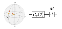
A concrete instance of this type is shown in Fig. 2. In this example, the angles with (Z-axis) of the two states and are and , respectively; see the first figure in Fig. 2. Around these two vectors, we randomly sample two sets (one for category “a” and one for category “b”) of quantum data points on the sphere, forming a dataset. The dataset consists of samples for the training and samples for the validation. As shown in Fig. 2, we use a parameterized rotation gate and a measurement to do the classification. Targeting to minimizing the MSE form of Eq. (8), we use Adam optimizer [39] to update . After training, we achieve both training and validation accuracy, and the final parameter is .
7.2 Quantum Phase Recognition
Quantum phase recognition (QPR) of one dimensional many-body systems has been attacked by quantum convolutional neural networks (QCNNs) proposed by Cong et al. [5]. Consider a symmetry-protected topological (SPT) phase and the ground states of a family of Hamiltonians on spin- chain with open boundary conditions:
where are Pauli matrices [2] for the spin at site , and the symmetry is generated by The goal is to identify whether the ground state of belongs to phase when is regarded as a function of . For small , a numerical simulation can be used to exactly solve this problem [5]; See Fig. 4a in Appendix E of the extended version of this paper [31] for the exact phase boundary points (blue and red diamonds) between SPT phase and non-SPT (paramagnetic or antiferromagnetic) phase for . Thus the -qubit instance is an excellent testbed for different new methods and techniques of QPR. Here, we train a QCNN model to implement -qubit QPR in this setting.
To generate the dataset for training, we sample a serials of Hamiltonian with , uniformly varying from to and compute their corresponding ground states; see the gray line of Fig. 4a in Appendix E of the extended version of this paper [31]. For the testing, we uniformly sample a set of validation data from two random regions of the 2-dimensional space ; see the two dashed rectangles of Fig. 4a. Finally, we obtain training data and validation data. Our parameterized QCNN circuit is shown in Fig. 4b in Appendix E of the extended version of this paper [31], and the unitaries are parameterized with generalized Gell-Mann matrix basis [40]: , where is a matrix and is a real number; the total number of parameters , is 114. For the outcome measurement of one qubit, we use measurement to predict that input states belongs to with output , where . Targeting to minimizing the MSE form of Eq. (8), we use Adam optimizer to update the parameters. After training, training accuracy and validation accuracy are obtained. At the same time, our classifier conducts a phase diagram (the colorful figure in Fig. 4a), where the learned phase boundary almost perfectly matches the exact one gotten by the numerical simulation. All these results indicate that our classifier is well-trained.
7.3 Cluster Excitation Detection
The task of cluster excitation detection is to train a quantum classifier to detect if a prepared cluster state is “excited” or not [7]. Excitations are represented with a rotation on one qubit. A large enough rotation is deemed to be an excited state and is labeled by , while a rotation that isn’t large enough is labeled by and is not deemed to be an excited state. Here, we demonstrate this classification task with qubits. We use the circuit shown in Fig. 5a of Appendix E in the extended version of this paper [31] to generate training () and validation () samples. The circuit generates cluster state by performing a rotation (we omit angle ) on one quibit. The rotation angle is ranging from to and if , the label of the output state is ; otherwise, the label is . The classification circuit model (a quantum convolutional neural network) uses the same structure in TensorFlow Quantum [7], shown in Fig. 5b of Appendix E in the extended version of this paper [31]. The explicit parameterization of can be found in [7]. The final measurement . Targeting to minimizing the MSE form of Eq. (8), we use Adam optimizer to update all . We achieve training accuracy and validation accuracy.
7.4 The Classification of MNIST
Handwritten digit recognition is one of the most popular tasks in the classical machine learning zoo. The archetypical training and validation data come from the MNIST dataset which consists of 55,000 training samples handwritten digits [41]. These digits have been labeled by humans as representing one of the ten digits from number 0 to 9, and are in the form of gray-scale images that contains pixels. Each pixel has a grayscale value ranging from to . Quantum machine learning has been used to distinguish a too simplified version of MNIST by downscaling the image sizes to pixels. Subsequently, the numbers represented by this version of MNIST can not be perceptually recognized [7]. Here, we build up a quantum classifier to recognize a MNIST version of pixels (see second column images of Fig. 3). As demonstrated in [7], we select out images of number and images of number to form our training () and validation () datasets. Then we downscale those images to images (fitting the size of quantum data), and encode them into the pure states of qubits via amplitude encoding. Amplitude encoding uses the amplitude of computational basis to represent vectors with normalization:
where is a set of orthogonal basis of the 8 qubits state space. The normalization doesn’t change the pattern of those images. For learning a quantum classifier, we use the QCNN model in Fig. 6 of Appendix E in the extended version of this paper [31] and use measurement . The output of measurement indicates the numbers: output for number and output for number . The explicit parameterization of those can be found in [7]. Again we use Adam optimizer to update the model parameters minimizing the MSE form of Eq.(8). We finally achieve training accuracy and validation accuracy.
7.5 Robustness Verification
Now, we start to check the -robustness for the above four well-trained classifiers presented in the previous four subsections.
In practical applications, the value of robustness in Definition 3 represents the ability of state preparation by quantum controls. For example, the state-of-the-art is that a single qubit can be prepared with fidelity 99.99% (e.g. [29, 30]). Here, we choose four different values of in each experiment.
| Robust Accuracy (in Percent) | ||||
| Robust Bound (Lemma 5.1 - Algorithm 3) | ||||
| Robustness Algorithm (Theorem 5.2 - Algorithm 2) | ||||
| Verification Times (in Seconds) | ||||
| Robust Bound (Lemma 5.1 - Algorithm 3) | ||||
| Robustness Algorithm (Theorem 5.2 - Algorithm 2) | ||||
To show the scalability of our robust bound given in Lemma 1, we use it to develop an algorithm (Algorithm 3 in Appendix F of the extended version of this paper [31]) to under-approximate the robust accuracy, which is computed by Algorithm 2. Algorithm 3 is a subroutine of Algorithm 2 without calling an SDP solver (whenever a potential non-robust state can be detected by the robust bound in Lemma 1). We compare the verification times by Algorithms 2 and 3.
The experiments are done on a computer with the following configurations: Intel(R) Core(TM) i7-9700 CPU @ 3.00GHz 8 Processor, 15.8 GiB Memory, Ubuntu 18.04.5 LTS, with CVXPY: Python Software for Disciplined Convex Programming [38] for solving SDP, and a SciPy solver for finding the minimum of constrained nonlinear multivariable function for solving QCQP.
| Robust Accuracy (in Percent) | ||||
| Robust Bound (Lemma 5.1 - Algorithm 3) | ||||
| Robustness Algorithm (Theorem 5.2 - Algorithm 2) | ||||
| Verification Times (in Seconds) | ||||
| Robust Bound (Lemma 5.1 - Algorithm 3) | ||||
| Robustness Algorithm (Theorem 5.2 - Algorithm 2) | ||||
The experimental results are given in Tables 1–4. As an example, we illustrate the details of the result for the case of in Table 1. First, we only apply our robust bound in Lemma 1 to pick up all potential non-robust states from the 800 points in the training dataset. Then points are left. Thus, the under-approximation of the robust accuracy computed by Algorithm 3 (in Appendix F of the extended version of this paper [31]) is 88.13%. Next, we check the -robustness by Algorithm 2. Indeed, only of the points detected by the above robust bound are non-robust and the exact robust accuracy is 90.00%. We also compare the verification time of the two approaches to the robust accuracy. See the second column in Table 1 for the detail, and other experiment results of -robustness are also summarized in the same table.
| Robust Accuracy (in Percent) | ||||
| Robust Bound (Lemma 5.1 - Algorithm 3) | ||||
| Robustness Algorithm (Theorem 5.2 - Algorithm 2) | ||||
| Verification Times (in Seconds) | ||||
| Robust Bound (Lemma 5.1 - Algorithm 3) | ||||
| Robustness Algorithm (Theorem 5.2 - Algorithm 2) | ||||
| Robust Accuracy (in Percent) | ||||
| Robust Bound (Lemma 5.1 - Algorithm 3) | ||||
| Robustness Algorithm (Theorem 5.2 - Algorithm 2) | ||||
| Verification Times (in Seconds) | ||||
| Robust Bound (Lemma 5.1 - Algorithm 3) | ||||
| Robustness Algorithm (Theorem 5.2 - Algorithm 2) | ||||
Tables 1–4 for the verification results show that in all of these experiments, the robust bound obtained in Lemma 1 scales very well, and the robustness verification by Algorithm 3 costs significantly less time () than the way of computing the optimal robust bound by Algorithm 2. For example, for quantum phase recognition, for and , the under-approximation of the robust accuracy is exactly same to the real value. Even for the last case of , only difference is got. Furthermore, from the tables, the verification time of Algorithm 2 is increasing with the value of , while the running time of the method by the robust bound is almost unchanged. This is because the former algorithm uses a SDP or QCQP solver to search all possible adversarial examples for the potential non-robust states picked up by the robust bound, and the number of these states are growing up with the value of . These counter-examples detected by the algorithm confirms that our robustness framework is effective. For instance, see Fig. 3 for two visualized adversarial examples generated by Algorithm 2 with a QCQP solver. As we can see, the benign and adversarial images are perceptually similar. This also proves that our robustness verification algorithm can detect not only quantum but also classical adversarial examples.


8 Conclusion
In this work, we initiate the research of the formal robustness verification of quantum machine learning algorithms against unknown quantum noise. We found an analytical robustness bound which can be efficiently computed to under-approximate the robust accuracy in practical applications. Furthermore, we developed a robustness verification algorithm that can exactly verify the -robustness of quantum machine learning algorithms and provides useful counter-examples for the adversarial training.
For topics for future research, it should be useful in practical applications to find an efficient method that over-approximates the robust accuracy of quantum classifiers. Combined the under-approximation approach developed in this work, it can help us to more accurately and fast estimate the robust accuracy. In classical machine learning, there exist some works in the literature to achieve this task. For instance, ImageStars, a new set representation, is introduced in [13] to perform efficient set-based analysis by combining operations on concrete images with linear programming, which leads to efficient over-approximative analysis of classical convolutional neural networks.
Tensor networks are one of the best-known data structures for implementing large-scale quantum classifiers (e.g. QCNNs with 45 qubits in [5]). For practical applications, we are going to incorporate tensor networks into our robustness verification algorithm so that it can scale up to achieve the demand of NISQ devices (of 50 qubits).
More generally, further investigations are required to better understand the role of the robustness in quantum machine learning, especially through more experiments on real world applications like learning phases of quantum many-body systems.
Acknowledgments
We would like to thank the anonymous reviewers for their insightful comments. This work was partly supported by the National Key R&D Program of China (Grant No: 2018YFA0306701), the National Natural Science Foundation of China (Grant No: 61832015) and the Australian Research Council (ARC) under grant No.DP210102449.
References
- [1] Giuseppe Carleo and Matthias Troyer. Solving the quantum many-body problem with artificial neural networks. Science, 355(6325):602–606, 2017.
- [2] Michael A Nielsen and Isaac L Chuang. Quantum computation and quantum information. Cambridge university press, 2010.
- [3] Jacob Biamonte, Peter Wittek, Nicola Pancotti, Patrick Rebentrost, Nathan Wiebe, and Seth Lloyd. Quantum machine learning. Nature, 549(7671):195–202, 2017.
- [4] Vedran Dunjko and Hans J Briegel. Machine learning & artificial intelligence in the quantum domain: a review of recent progress. Reports on Progress in Physics, 81(7):074001, 2018.
- [5] Iris Cong, Soonwon Choi, and Mikhail D Lukin. Quantum convolutional neural networks. Nature Physics, 15(12):1273–1278, 2019.
- [6] Hsin-Yuan Huang, Richard Kueng, and John Preskill. Information-theoretic bounds on quantum advantage in machine learning. arXiv preprint arXiv:2101.02464, 2021.
- [7] Michael Broughton, Guillaume Verdon, Trevor McCourt, Antonio J Martinez, Jae Hyeon Yoo, Sergei V Isakov, Philip Massey, Murphy Yuezhen Niu, Ramin Halavati, Evan Peters, et al. Tensorflow quantum: A software framework for quantum machine learning. arXiv preprint arXiv:2003.02989, 2020. See https://www.tensorflow.org/quantum for the platform.
- [8] Ling Huang, Anthony D Joseph, Blaine Nelson, Benjamin IP Rubinstein, and J Doug Tygar. Adversarial machine learning. In Proceedings of the 4th ACM workshop on Security and artificial intelligence, pages 43–58, 2011.
- [9] Ian J. Goodfellow, Jonathon Shlens, and Christian Szegedy. Explaining and harnessing adversarial examples. In Yoshua Bengio and Yann LeCun, editors, 3rd International Conference on Learning Representations, ICLR 2015, San Diego, CA, USA, May 7-9, 2015, Conference Track Proceedings, 2015.
- [10] Aleksander Madry, Aleksandar Makelov, Ludwig Schmidt, Dimitris Tsipras, and Adrian Vladu. Towards deep learning models resistant to adversarial attacks. In 6th International Conference on Learning Representations, ICLR 2018, Vancouver, BC, Canada, April 30 - May 3, 2018, Conference Track Proceedings. OpenReview.net, 2018.
- [11] Nicholas Carlini and David Wagner. Adversarial examples are not easily detected: Bypassing ten detection methods. In Proceedings of the 10th ACM Workshop on Artificial Intelligence and Security, pages 3–14, 2017.
- [12] Tom B Brown, Dandelion Mané, Aurko Roy, Martin Abadi, and Justin Gilmer. Adversarial patch. arXiv preprint arXiv:1712.09665, 2017.
- [13] Hoang-Dung Tran, Stanley Bak, Weiming Xiang, and Taylor T Johnson. Verification of deep convolutional neural networks using imagestars. In International Conference on Computer Aided Verification, pages 507–526. Springer, 2020.
- [14] Yizhak Yisrael Elboher, Justin Gottschlich, and Guy Katz. An abstraction-based framework for neural network verification. In International Conference on Computer Aided Verification, pages 43–65. Springer, 2020.
- [15] Daniel J Fremont, Johnathan Chiu, Dragos D Margineantu, Denis Osipychev, and Sanjit A Seshia. Formal analysis and redesign of a neural network-based aircraft taxiing system with verifai. In International Conference on Computer Aided Verification, pages 122–134. Springer, 2020.
- [16] Marta Z. Kwiatkowska. Safety verification for deep neural networks with provable guarantees (invited paper). In Wan J. Fokkink and Rob van Glabbeek, editors, 30th International Conference on Concurrency Theory, CONCUR 2019, August 27-30, 2019, Amsterdam, the Netherlands, volume 140 of LIPIcs, pages 1:1–1:5. Schloss Dagstuhl - Leibniz-Zentrum für Informatik, 2019.
- [17] Tommaso Dreossi, Daniel J Fremont, Shromona Ghosh, Edward Kim, Hadi Ravanbakhsh, Marcell Vazquez-Chanlatte, and Sanjit A Seshia. Verifai: A toolkit for the formal design and analysis of artificial intelligence-based systems. In International Conference on Computer Aided Verification, pages 432–442. Springer, 2019.
- [18] Hoang-Dung Tran, Xiaodong Yang, Diego Manzanas Lopez, Patrick Musau, Luan Viet Nguyen, Weiming Xiang, Stanley Bak, and Taylor T Johnson. Nnv: The neural network verification tool for deep neural networks and learning-enabled cyber-physical systems. In International Conference on Computer Aided Verification, pages 3–17. Springer, 2020.
- [19] Sirui Lu, Lu-Ming Duan, and Dong-Ling Deng. Quantum adversarial machine learning. Phys. Rev. Research, 2:033212, Aug 2020.
- [20] Yuxuan Du, Min-Hsiu Hsieh, Tongliang Liu, Dacheng Tao, and Nana Liu. Quantum noise protects quantum classifiers against adversaries. arXiv preprint arXiv:2003.09416, 2020.
- [21] Nana Liu and Peter Wittek. Vulnerability of quantum classification to adversarial perturbations. Physical Review A, 101(6):062331, 2020.
- [22] Maurice Weber, Nana Liu, Bo Li, Ce Zhang, and Zhikuan Zhao. Optimal provable robustness of quantum classification via quantum hypothesis testing. arXiv preprint arXiv:2009.10064, 2020.
- [23] Carl W Helstrom. Detection theory and quantum mechanics. Information and Control, 10(3):254–291, 1967.
- [24] Mahmood Sharif, Lujo Bauer, and Michael K Reiter. On the suitability of lp-norms for creating and preventing adversarial examples. In Proceedings of the IEEE Conference on Computer Vision and Pattern Recognition Workshops, pages 1605–1613, 2018.
- [25] T Figueiredo Roque, Aashish A Clerk, and Hugo Ribeiro. Engineering fast high-fidelity quantum operations with constrained interactions. npj Quantum Information, 7(1):1–17, 2021.
- [26] Boyan T Torosov and Nikolay V Vitanov. Smooth composite pulses for high-fidelity quantum information processing. Physical Review A, 83(5):053420, 2011.
- [27] Edward Farhi, Hartmut Neven, et al. Classification with quantum neural networks on near term processors. Quantum Review Letters, 1(2 (2020)):10–37686, 2020.
- [28] Seunghyeok Oh, Jaeho Choi, and Joongheon Kim. A tutorial on quantum convolutional neural networks (qcnn). In 2020 International Conference on Information and Communication Technology Convergence (ICTC), pages 236–239. IEEE, 2020.
- [29] AH Myerson, DJ Szwer, SC Webster, DTC Allcock, MJ Curtis, G Imreh, JA Sherman, DN Stacey, AM Steane, and DM Lucas. High-fidelity readout of trapped-ion qubits. Physical Review Letters, 100(20):200502, 2008.
- [30] AH Burrell, DJ Szwer, SC Webster, and DM Lucas. Scalable simultaneous multiqubit readout with 99. 99% single-shot fidelity. Physical Review A, 81(4):040302, 2010.
- [31] Ji Guan, Wang Fang, and Mingsheng Ying. Robustness verification of quantum classifiers. arXiv preprint arXiv:2008.07230, 2020.
- [32] Wenjie Ruan, Min Wu, Youcheng Sun, Xiaowei Huang, Daniel Kroening, and Marta Kwiatkowska. Global robustness evaluation of deep neural networks with provable guarantees for the hamming distance. In Sarit Kraus, editor, Proceedings of the Twenty-Eighth International Joint Conference on Artificial Intelligence, IJCAI 2019, Macao, China, August 10-16, 2019, pages 5944–5952. ijcai.org, 2019.
- [33] Alessio Lomuscio and Lalit Maganti. An approach to reachability analysis for feed-forward relu neural networks. arXiv preprint arXiv:1706.07351, 2017.
- [34] Vincent Tjeng, Kai Y. Xiao, and Russ Tedrake. Evaluating robustness of neural networks with mixed integer programming. In 7th International Conference on Learning Representations, ICLR 2019, New Orleans, LA, USA, May 6-9, 2019. OpenReview.net, 2019.
- [35] Osbert Bastani, Yani Ioannou, Leonidas Lampropoulos, Dimitrios Vytiniotis, Aditya V. Nori, and Antonio Criminisi. Measuring neural net robustness with constraints. In Daniel D. Lee, Masashi Sugiyama, Ulrike von Luxburg, Isabelle Guyon, and Roman Garnett, editors, Advances in Neural Information Processing Systems 29: Annual Conference on Neural Information Processing Systems 2016, December 5-10, 2016, Barcelona, Spain, pages 2613–2621, 2016.
- [36] Richard Y Zhang and Javad Lavaei. Sparse semidefinite programs with near-linear time complexity. In 2018 IEEE Conference on Decision and Control (CDC), pages 1624–1631. IEEE, 2018.
- [37] Guy Katz, Clark Barrett, David L Dill, Kyle Julian, and Mykel J Kochenderfer. Reluplex: An efficient smt solver for verifying deep neural networks. In International Conference on Computer Aided Verification, pages 97–117. Springer, 2017.
- [38] Steven Diamond and Stephen Boyd. CVXPY: A Python-embedded modeling language for convex optimization. Journal of Machine Learning Research, 17(83):1–5, 2016.
- [39] Diederik P. Kingma and Jimmy Ba. Adam: A method for stochastic optimization. In Yoshua Bengio and Yann LeCun, editors, 3rd International Conference on Learning Representations, ICLR 2015, San Diego, CA, USA, May 7-9, 2015, Conference Track Proceedings, 2015.
- [40] Reinhold A Bertlmann and Philipp Krammer. Bloch vectors for qudits. Journal of Physics A: Mathematical and Theoretical, 41(23):235303, may 2008.
- [41] Yann LeCun and Corinna Cortes. MNIST handwritten digit database. http://yann.lecun.com/exdb/mnist/, 2010.
- [42] Koenraad MR Audenaert, John Calsamiglia, Ramón Munoz-Tapia, Emilio Bagan, Ll Masanes, Antonio Acin, and Frank Verstraete. Discriminating states: The quantum chernoff bound. Physical review letters, 98(16):160501, 2007.
- [43] Robin J Blume-Kohout. How distinguishable are two quantum processes? or what is the error rate of a quantum gate? Technical report, Sandia National Lab.(SNL-NM), Albuquerque, NM (United States), 2017.
- [44] John Watrous. Semidefinite programs for completely bounded norms. Theory Comput., 5(1):217–238, 2009.
- [45] Sunyoung Kim and Masakazu Kojima. Exact solutions of some nonconvex quadratic optimization problems via sdp and socp relaxations. Computational optimization and applications, 26(2):143–154, 2003.
Appendix
Appendix 0.A Fidelity v.s. Trace Distance
In this section, we give more details of the reason that fidelity is better than trace distance as the metric in the study of the robustness of quantum machine learning against quantum noise.
As we know, a quantum computation can be modeled by a super-operator [2]. Under quantum noise, is disturbed to be another super-operator . How to measure the disturbance with some metric ? We have to apply them to a quantum system prepared in a state . Then we obtain the optimal discrimination by maximizing over :
| (9) |
where is some metric of state distinguishability. So we need to find a good metric of state distinguishability. Of all good candidates, fidelity and trace distance are two of the most widely used metrics.
Trace distance quantifies the maximum probability of correctly guessing whether or was prepared after making a measurement [2]:
where
is the trace distance between and , and is trace norm. Thus when copies of and are provided,
So how does behave as tends to infinite as the scenario of quantum machine learning? The quantum Chernoff bound explains this [42]:
where is a non-zero positive constant and is the quantum Chernoff bound which is generally hard to be computed. And when the states are pretty close, it’s close to the infidelity (1-) [43]:
Therefore, let be a small enough threshold value,
where . In terms of trace distance, we have:
which is derived by the Fuchs-van de Graaf inequalities
By the above inequalities about , we can see that infidelity gives a better (linear) estimation of how many samples we need to accurately discriminate from than trace distance which gives a polynomial estimation of . For instance, when (then ), for the same value of infidelity and trace distance, saying , the estimations of is and , respectively. Thus fidelity is more suitable as the metric in Eq.(9) in the scenario of quantum machine learning that many copies of quantum states are provided.
Appendix 0.B Proof of Lemma 5.1
Proof
For any with , by the monotonicity of the fidelity [2, Theorem 9.6], we have
Let
Without loss of generality, we assume . We use and to denote the inner product of and the -norm, respectively. Then and both have unit norms:
By the definition of fidelity, we have
We see that any probability distribution with and can be viewed as a unit vector and the fidelity of two distributions is the inner product of their corresponding unit vectors.
Next, we prove that the unit vector form of can be used to obtain a robust bound for it. First, we find a vector that has maximum inner product with and is within another class rather than the belonging class of . This can be done by solving the following optimization problem:
| (10) |
With constraint , we have for any . Thus, let , the above optimization problem is rewritten as:
| (11) |
The objective function is not changed by multiplying the numerator and denominator with a positive number. Thus, we can assume and obtain the following problem
| (12) |
By the assumption of , we claim that the constraint
can be replaced by . Suppose the optimal solution is
Then let
For the case of , with , we have
then there exists such that
which is equivalent to
So the first and second elements of are equal.
We have
which means that and are orthogonal. Then
We find a vector satisfies and .
Now we consider the situation of . We have and , and following the same analysis in the above, we can find such that the second and -th elements of are equal and
which is contradict to is the optimal value. Thus, the optimal value is achieved at a vector satisfying , then the problem can be reformulated as
| (13) |
Using the Lagrange multiplier method, the optimal value of problem (13) is
Then the optimal value of problem (10) is
Therefore, if
then for any vector with , we have the corresponding quantum state with and is classified into the class of . In other words, is -robust.
Appendix 0.C Proof of Theorem 5.1
Proof
The sufficient direction directly follows from the definition of adversarial robustness in Definition 3. For the necessary direction, if there is such that there is a solution in the above problem, then , i.e., is classified in the class . That is is an -adversarial example of and is not -robust.
Now we prove that the above problem can be reduced to a SDP. First, it is easy to verify , the set of quantum states on , is a convex set of positive semidefinite matrices. Computing can be reduced to solving a SDP [44]. Thus replacing by the SDP, the above problem is a SDP problem by noting that is equivalent to and .
Appendix 0.D Pure State Robustness Verification
In this section, we discuss the robustness verification for pure states, i.e. pure state against adversarial examples of pure states. That is that all quantum states in the training dataset and their adversarial examples are pure states. Then, by Theorem 5.2 and noting that the set of all pure states is not convex, computing the optimal robust bound for pure states is not an SDP. But we can prove it is a Quadratically Constrained Quadratic Program (QCQP), which is hard to be solved.
In mathematical optimization, a QCQP is an optimization problem in which both the objective function and the constraints are quadratic functions. It has the form
| subject to | |||
where are matrices and is the optimization variable. The problem is convex, if are all positive semidefinite, but non-convex, if these matrices are neither positive nor negative semidefinite. In general, solving QCQP is an NP-hard problem.
Corollary 1 (Pure State Optimal Robust Bound)
be a quantum classifier and is a pure state with . Then is the optimal robust bound of pure state against adversarial examples of pure states, where and is the solution of the following QCQP:
| subject to | |||
where if the QCQP is unsolved, then
Proof
First, we note that and for any matrix . Then the result follows from Theorem 5.2 and the observation that is equivalent to
where is the identity matrix on .
As we can see, the above QCQP is non-convex, so we cannot efficiently compute the pure state optimal robust bound like the mixed state case by SDP. However, there are some numerical tools designed to solve QCQP—not only compute the minimal value but also output a corresponding optimal solution , as SDP solvers. Some methods have been developed to approximately solving non-convex QCQPs in a reasonable time. For example, non-convex QCQPs with non-positive off-diagonal elements can be exactly solved by SDP relaxations [45]. Therefore, there may have a polynomial-time algorithm to solve this specific form of QCQP, and we left this problem as a future research.
Appendix 0.E Training Models
