Disentangled Item Representation for Recommender SystemsJournal: JACMVolume: 3741118CCS: Applied computing Online shoppingJournal: TISTVolume: 1111Price: 15.00DOI: 10.1145/3445811
Abstract.
Item representations in recommendation systems are expected to reveal the properties of items. Collaborative recommender methods usually represent an item as one single latent vector. Nowadays the e-commercial platforms provide various kinds of attribute information for items (e.g., category, price and style of clothing). Utilizing these attribute information for better item representations is popular in recent years. Some studies use the given attribute information as side information, which is concatenated with the item latent vector to augment representations. However, the mixed item representations fail to fully exploit the rich attribute information or provide explanation in recommender systems. To this end, we propose a fine-grained Disentangled Item Representation (DIR) for recommender systems in this paper, where the items are represented as several separated attribute vectors instead of a single latent vector. In this way, the items are represented at the attribute level, which can provide fine-grained information of items in recommendation. We introduce a learning strategy, LearnDIR, which can allocate the corresponding attribute vectors to items. We show how DIR can be applied to two typical models, Matrix Factorization (MF) and Recurrent Neural Network (RNN). Experimental results on two real-world datasets show that the models developed under the framework of DIR are effective and efficient. Even using fewer parameters, the proposed model can outperform the state-of-the-art methods, especially in the cold-start situation. In addition, we make visualizations to show that our proposition can provide explanation for users in real-world applications.
Keywords:
Representation learning, Recommender systems, Attribute disentangling1. Introduction
The item representations are significant in recommendation systems, which are expected to reveal the item properties. Early collaborative recommender methods represent an item as a single latent vector only using collaborative information (Rendle et al. 2009; Koren et al. 2009; Zhang et al. 2019). Today’s e-commercial platforms provide various kinds of attribute information for items (e.g., category, price and style of clothing) helping customers select their favorite items. These attribute information of items is significant but have not been fully exploited in recommender systems. Utilizing these information for better recommendation is preferred in recent years. For example, based on traditional collaborative methods, researchers try to add more attribute information to augment the representations (Lian et al. 2014; He and McAuley 2016b), by simply concatenating the attribute information with the latent item vectors and learning item representations by user-item interactions. Recently, some methods on clothing recommendation begin to analyze items from two attributes, i.e., category and style (He et al. 2016; Liu et al. 2017; Yu et al. 2018). Their success inspires us that an item could be considered as a combination of different attributes. Compared with item-level representations, attribute-level representations provide a more informative description for items.
In this paper, we formalize an novel item representation framework at the attribute level, Disentangled Item Representation (DIR), as shown in Figure 1. Each item is represented as a combination of attribute vectors instead of a single latent vector. Aside from the given attributes of items (generally called explicit attributes), we introduce an implicit attribute to distinguish items from those having the same given attributes. To better illustrate our framework, we take items of two explicit attributes for example. Assume the clothes have two kinds of given attributes, category and style. As shown in Figure 1, each item can be allocated into a cell of the 3-axes tensor, where each axis corresponds to one kind of attribute (2 explicit attributes and 1 implicit attribute). Accordingly, we have two main tasks: 1) assign each item with its corresponding implicit attribute (the explicit attribute are given), i.e., allocate each item into a cell of the tensor; 2) learn all the attribute vectors. We also introduce a learning algorithm, LearnDIR, in which we first randomly initialize all the attribute vectors and allocate them to items, and then we train the vectors and reallocate them to items alternately during training process.

DIR has several advantages compared with traditional methods. On one hand, DIR reduces the size of parameters. For a table with rows and columns, using latent attribute vectors, DIR can represent items at most. In pervious traditional models, the number of latent vectors equals the number of items (i.e., in the Figure 1) at least. On the other hand, DIR alleviates the cold-start problem. Cold-start items seldom appear on history records, indicating sparse collaborative information at the item level. However, DIR models items by shared attributes, where collaborative information is dense. DIR could be used in most collaborative recommender models. In this paper, we apply DIR on two typical models (i.e., MF and RNN). The proposed models are accordingly called DIR-MF and DIR-RNN. Experimental results on two real-world datasets show that the models developed under the framework of DIR are effective and efficient. Even using fewer parameters, the proposed model can outperform the state-of-the-art methods. In addition, we make visualizations to show that our proposition can provide the explainability for users in real-world applications.
Overall, main contributions of our work are summarized as follows:
- •
We propose a novel disentangled item representation for recommender systems, which can fully reveal the properties of items and provide explanation for making recommendation.
- •
DIR can reduce the size of parameters. It is a good solution to relieve the cold-start problem by taking advantage of the attribute sharing mechanism.
- •
We show how to implement DIR on two typical models, MF and RNN and demonstrate that DIR can represent items effectively and efficiently. Extensive experiments on real-world datasets show that our proposed DIR-RNN model outperforms the state-of-the-art methods.
2. Related Work
In this section, we briefly review some related works on representation learning and collaborative recommender methods for implicit feedback.
2.1. Disentangled Representation Learning
The representation learning algorithms are mainly discussed in natural language processing. The word embedding techniques achieve a great success, such as Word2Vec (Mikolov et al. 2013a; Mikolov et al. 2013b) and Glove (Pennington et al. 2014). Recently, LightRNN (Li et al. 2016) models the items’ commonalities based on the 2-component shared embedding, which largely reduces the parameter size. This work disentangles the word representations into two components at the first time and achieves considerable performance. Many researchers begin to realize the significance of representation disentangling. Disentangled representation is commonly the idea of analyzing different attributes of image or text. Michael et al (Mathieu et al. 2016) and Xi Chen et al (Chen et al. 2016) try to split the style information from image by representation disentangling. Vineet et al (John et al. 2018) use the auto-encoder model to disentangle the sentiment information of text. Not only in the area about image or text, disentangled representations can capture the descriptive entity (Higgins et al. 2018) of the real world. In e-commercial applications, items representation could be disentangled as attributes, which may bring the bonus for recommendation.
2.2. Item Representation Learning
In recommendation applications, previous researchers enrich the item representation by using more attribute information. The work of (Lian et al. 2014) simply augments the item representation by concatenating location information with latent factors. Sun et al (Sun et al. 2017b) uses the information of the category tree to give item hierarchical representation. These works try to augment the item representation by using attribute information to describe items more elaborately. Some works also begin to analyze the items’ attributes in detail. For example, in clothing recommendation, researchers describe items from the view of category and style (McAuley et al. 2015). He et al (He et al. 2016) and Liu et al (Liu et al. 2017) hold the view that both category and style reflect properties of items together. Sherlock (He et al. 2016) uses well-designed linear projections to get style representations from visual information, where different categories of items have different projections. DeepStyle (Liu et al. 2017) declares that style representation could be obtained by splitting category information from visual representation. Following the ideas above, some recent works map items into different attribute spaces to get multiple views of items. For example, Yu et al (Yu et al. 2018) extract both aesthetic features and category features from item images to represent items in aesthetic space and category space. Sun et al (Sun et al. 2017a; Sun et al. 2017b) try to model the category tree to get different item representations in different hierarchical spaces. Recently, some researches on fashion recommendation begin to adopt more attribute tags (Bao et al. 2019; Yang et al. 2019; Hou et al. 2019) and content information (Hu et al. 2019; Yan et al. 2019; Shin et al. 2019) to enrich items. Different from previous works, our proposed model directly represents items by their attributes. Each item has a disentangled representation at the attribute level.
2.3. Collaborative Methods for Implicit Feedback
Implicit feedbacks come from the users’ behavior on the internet, which could be tracked automatically, such as clicks, purchases, and so on. Compared with explicit feedbacks like ratings, implicit feedbacks are easier to be collected, but more difficult to be modeled because of containing only positive observations. Collaborative recommender models are mainly used for implicit feedback. Matrix factorization (MF) (Koren et al. 2009) is a classical collaborative method. Especially, One-Class MF (Pan et al. 2008) treats the non-observed interactions as negative samples. After that, Bayesian Personalized Ranking (BPR) (Rendle et al. 2009) is introduced, using pair-wise ranking strategies to balance the positive and negative samples. By using the BPR framework, BPR-MF achieves the state-of-the-art performance in many scenarios.
Since then, some works try to apply BPR to sequential recommendation. For example, Factorizing Personalized Markov Chains (FPMC) (Rendle et al. 2010) uses Markov Chains to model sequential behaviors of users and employs BPR to learn the factorization parameters. Recently, some researchers begin to use RNN to model the sequential behaviors (Yu et al. 2016; Liu et al. 2016a). Long Short-Term Memory (LSTM) (Hochreiter and Schmidhuber 1997; Gers et al. 2000; Sundermeyer et al. 2012) is a popular RNN architecture, which can alleviate the long-term dependence problem of RNN. Various RNN based models tend to use LSTM for recommendation.
3. Proposed Method
In this section, we first give the basic notation used in this paper and then propose DIR which could be used for collaborative recommendation models. After that, we introduce LearnDIR for DIR learning. Finally, we show how DIR can be combined with two typical models, MF and RNN.
3.1. Notation
We use a tuple to describe the user behavior, which means that a user buys an item . Let be the set of all users and be the set of all items. The purchase set could be formalized as . The task of the recommender algorithms is to provide each user with a personalized score on each item , denoted as . The larger value of , the higher probability that buy . For convenience, we also define:
where is the set of items which are purchased by the user , and is the set of users who have purchased the item .
3.2. Disentangled Item Representation
We formulate that an item is represented by the combination of several explicit attributes (given) and an implicit attribute (unknown). There are kinds of explicit attributes noted as,
Each explicit attribute represents a known attribute. The implicit attribute is noted as,
implicit attributes is defined to describe the latent attribute of items, which is not described by explicit attributes. By adding implicit attributes, items with the same explicit attributes could be distinguished from each other. We pre-define the number of implicit attributes for a specific dataset to guarantee each item belongs a unique combination (detail discussion in Section 4.6.2). We have two tasks: 1) allocate attributes to items and 2) learn all the attribute vectors and . Mathematically, we use allocating functions (or ) to formulate whether belongs to an explicit attribute (or an implicit attribute ). means that the item belongs to the attribute , otherwise , and has the same analogous definition. Task 1 could be considered as allocating each item into a cell of a tensor with axes (i.e., explicit attributes and implicit attribute). In the following, Equation (1) makes sure that each cell of the tensor could have at most one item. Equation (2) guarantees that each item could only be allocated to one cell of the tensor. Satisfying both Equations of constraints, each item could be uniquely represented.
| (1) |
| (2) |
We denote the preference of user for explicit attribute and implicit attribute as and . Given a user behavior tuple (, ), instead of predicting directly, we predict his preference for attributes respectively. can be formulated as:
| (3) |
where item is represented by . Commonly, preference indicts the favor degrees of a user for items. In this paper, we extend the meaning of preference, which indicts the favor degrees of a user for attributes. In that case, the favor degrees of a user to an item (i.e., ) could be considered as the aggregation of the preference of for all the attributes that possesses. Here, we use multiply as aggregation for simplification.
3.3. LearnDIR
LearnDIR aims to minimize the negative log loss, which is formulated as,
| (4) | ||||
Since the explicit attributes are given in most e-commercial scenarios, the allocation of items is usually known11 1 We set this constraint for the reason that most recommender applications have explicit attributes information. Adding this constraint could make a great profit on performance. Without this constraint, the following optimization could still be done in the same way. Detail discussions are in Section 4.4.. We simplify our learning algorithm to only deal with the implicit attribute allocation . Different from other parameters, the allocating function is non-differentiable. We thus take a bootstrap strategy (Li et al. 2016) by iteratively conducting E-step and R-step. E-step mainly deals with estimating all latent attribute vectors, and . R-step aims to find a better implicit attribute allocation , since is known (that is because the explicit attributes of an item are always known). The LearnDIR algorithm is shown in Algorithm 1. Initially, we give each item a random implicit attribute. Then, we iteratively conduct E-step and R-step until the convergence.
E-step: Estimating latent vectors. This step assumes that the allocating function is given. With the fixed , we train the specific model (e.g. MF, RNN) with DIR to learn the latent vectors of attributes. The specific model estimates latent vectors of the explicit and implicit attributes, along with and , which will be described in Section 3.5 in detail. Generally, the gradient of our loss function with respect to the model parameters is,
| (5) |
We use stochastic gradient descent (SGD) to learn the parameter in E-step. In this case, for each user-item pair , an update is performed.
| (6) |
where is the learning rate of SGD. We stochastically update parameters by user-item pairs in the training set. The loss will converge after several epochs.
R-step: Reallocating items to implicit attributes. This step fixes and , which are estimated in E-step. Since usually does not need to be learned, we remove the explicit part in Equation (4), which leads to,
| (7) | ||||
Considering the constraints described in Equations (1) and (2), the complete optimization problem can be summarized as,
| (8) | ||||
where denotes the set of items having the same combination of explicit attributes .
For each , we use the OR-tool22 2 https://developers.google.com/optimization/; we use the solver of minimizing cost flow. to solve this optimization as finding a maximum matching between the item set and the implicit attribute set .
3.4. Model discussion
The time complexity of R-step is (Ahuja 2017), where is the number of latent vectors of implicit attributes. The training procedure could be conducted off-line, where the time consumption is acceptable. Both E-step and R-step share the same objective function. The only difference is E-step optimizes continuous variables, and R-step optimizes discrete variables. Since both step has the same objective function, they will promote each other. Similar strategies have been used in different application. (Li et al. 2016; McAuley and Leskovec 2013) We do experiments in Section 4.6.4 for further discussion.
DIR framework largely cuts down the parameters of item representation and does not bring much time complexity during inference. However, the drawback of DIR based methods is the time complexity in training process. The training process is much longer than original methods. The main problem comes from the difficulty of allocating items into suitable attributes (i.e., MCMF). In real-world application, we could give a good initialization of allocation according to prior knowledge or previous training results. Besides, the inference time of DIR is similar to item based representation models, which makes DIR workable.
DIR framework could alleviate the cold-start problem to a certain extent without adding other content information. In common collaborative methods, the cold-start problem partly comes from too sparse collaborative information of new items. It is difficult for new items to have accurate representations, since there are few collaborative information for optimization. However, under the framework of DIR, all items are represented at attribute level, which means items share attribute vectors with others, so that a new item could share well-learnt attributes vectors of other old items. We can learn how to best represent or allocate new items based on the already well-learned attributes in R-step, which only need a few collaborative records.
3.5. Learning Models with DIR
DIR is a model-agnostic attributed based item representation framework. All the collaborative filtering based methods who represent items as vectors and calculate for recommendation could be used under DIR. In this subsection, we describe two typical recommender models, MF and RNN, and show how we can learn these two models with DIR. Both MF and RNN try to predict the possibility of a user purchasing an item. For MF, the prediction is a score per user-item pair . For RNN, the prediction is per user-item-time tuple . Instead of modeling an item by a latent vector in original MF and RNN, we provide a latent vector for each attribute and model items by a combination of attribute vectors in the DIR framework.
MF with DIR. To predict the rating score of user on item , MF represents both users and items in a joint latent vector space, such that the user-item interaction is modeled as the inner product in that space (Koren et al. 2009).
In DIR, MF could model the preference of user u for explicit and implicit attribute by dot product as
| (9) |
According to Equations (4) and (9), the objective function in DIR-MF is expressed as,
| (10) |
RNN with DIR. RNN can capture the sequential structure of the user historical behavior. To describe RNN for recommendation, we formulate to denote the item which is bought by at time step . The behavior set is formed by the triple which means purchases at time step .
In the RNN recommender model (Yu et al. 2016; Liu et al. 2016b; Cui et al. 2019), the input sequence of RNN is the item representation of the item . At time step , we calculate the hidden layer by the input and the hidden layer at the previous time step . The hidden layer can be treated as the dynamic representation of the user . The following equation denotes a unit of RNN,
| (11) |
where , are transition parameter matrices and is the activation function (e.g., the sigmoid function ).
In DIR-RNN, we concatenate the attribute vectors to represent the corresponding item . That is to say,
| (12) |
where the item belongs to the explicit attribute and implicit attribute .
At each time step, the preference of user for explicit and implicit attributes could be determined by dot product,
| (13) |
4. Experiments
The main contribution of this work is to develop a new representation method DIR for recommendation. We aim to answer the following research questions via experiments.
-
RQ1 Does the method under the DIR framework perform better than other methods?
-
RQ2 Does the method under the DIR framework perform better than other methods in cold-start situation?
-
RQ3 Does the improvement of performance come from the disentangled representation at the attribute level?
-
RQ4 How does the learned attribute representation guide the real-world application?
-
RQ5 How do different parts of DIR affect the performance and how does DIR work?
Next, we first describe the experimental settings. We then report results by answering the above research questions in turn.
| Dataset | # Users | # Items | # Category | # Feedback | % Cold-start |
|---|---|---|---|---|---|
| Clothing | 20196 | 22280 | 323 | 145932 | 34.25 |
| Electronics | 15944 | 28519 | 281 | 117485 | 22.25 |
4.1. Experimental Settings
Datasets: We use the amazon dataset33 3 http://jmcauley.ucsd.edu/data/amazon/links.html (McAuley et al. 2015; He and McAuley 2016a) to assess the performance of our proposed method. We choose the “Clothing Shoes & Jewelry” and the “Electronics” datasets, which are named as Clothing and Electronics for short. Following the previous work (Sun et al. 2017a), we uniformly sample the datasets to balance their sizes for the cross-dataset comparison. Following the work of (Liu et al. 2017), we remove users with less than 5 purchases or more than 100 purchases. The statistics of datasets are listed in Table 1. Items which appear less than 5 times in the training data are called cold-start items. The percent of cold-start items is of overall testing set in Clothing, while in Electronics. We evaluate all methods with two settings in the following sections: Warm-start and Cold-start. The warm-start setting focuses on the overall ranking performance using the whole test set, while the cold-start setting only uses cold-start items in the test set.
Parameter Settings: Since category is the only completely given attribute from these two datasets, we only consider one explicit attribute (i.e., category) in our experiment. In both DIR-MF and DIR-RNN, we initially set the learning rate as 1.0 and then decrease it by a ratio of 2 after ten epochs. In our experiment, the number of implicit attributes is 1584 in the Clothing dataset, and 2958 in the Electronics dataset. The number of latent vectors of implicit attributes is equal to the number of items in the largest category, which is the least number of implicit attributes to guarantee that every item has a distinctive combination (detail discussion in Section 4.6.2). In order to have a better category representation, we embed categories in a hierarchical way, similar to Sherlock (He et al. 2016), which has been proved effective and efficient.
Evaluation Protocol: Similar to several previous works of recommendations with implicit feedback (Rendle et al. 2009; He et al. 2016), we also use the leave-one-out protocol for evaluation. For each user , we use the last purchase for testing and the others for training. We apply the average AUC (Area Under the ROC Curve) metric to evaluate the performance of all methods in terms of personalized ranking,
| (15) |
where is the leave-out item that the user purchases, is a random item that the user hasn’t purchased, is the indicator function which equals to one when the condition is met, and zero otherwise.
Compared methods: we compare the proposed model with the following methods:
- •
MF (Rendle et al. 2009) is required as BPR-MF which is known as a classical MF method for implicit feedback.
- •
FPMC (Rendle et al. 2010) combines Markov chain and MF for sequential recommendation.
- •
RNN (Yu et al. 2016) here denotes the LSTM-based RNN model, which alleviates the long-term dependencies of basic RNN.
- •
Sherlock (He et al. 2016) uses both hierarchical category information and visual information to enhance the item embeddings.
- •
HieVH (Sun et al. 2017a) models the item relationship using hierarchical category information.
| Dataset | Setting | MF | FPMC | RNN | Sherlock | HieVH | DIR-MF | DIR-RNN |
|---|---|---|---|---|---|---|---|---|
| Clothing | warm-start | 0.5842 | 0.6766 | 0.6784 | 0.7065 | 0.7401 | 0.6549 | 0.7569 |
| # parameter (M) | 1.3003 | 6.1533 | 1.1342 | 12.2634 | 496.8363 | 1.1373 | 0.2886 | |
| time (s) | 0.1134 | 0.2932 | 120.3526 | 0.2767 | 1.1592 | 0.2738 | 178.1951 | |
| Electronics | warm-start | 0.7061 | 0.7964 | 0.7517 | 0.7492 | 0.8217 | 0.7585 | 0.8548 |
| # parameter (M) | 1.3339 | 5.0751 | 1.4462 | 7.7214 | 816.0235 | 0.7594 | 0.2720 | |
| time (s) | 0.0806 | 0.1835 | 45.8593 | 0.2418 | 0.8251 | 0.2379 | 59.1175 |
4.2. Performance Comparison (RQ1)
We list the best performance, parameter size and the corresponding inference time of each method in Table 2. First of all, we can see that DIR-MF and DIR-RNN significantly improve the performance of both MF and RNN, which illustrates that DIR can well describe item properties for different recommendation models. Among the compared models, FPMC and RNN are both sequential recommendation models, and perform well in two datasets. Although HieVH achieves a relatively higher AUC in both datasets, it needs a complicated pre-training for item co-occurrence matrix consuming too much parameter space, which is difficult to use in real-world applications. Sherlock is highly dependent on the representativeness of visual information, so it performs well only in the Clothing dataset, and relatively poor in the Electronic dataset where visual information has difficulty in revealing attributes. Different from these methods, DIR-based models are not dependent on visual information. They perform stably in different datasets. Especially, DIR-RNN outperforms all other methods in terms of the prediction quality, which illustrates the ability of DIR. In term of evaluation time, DIR-MF consumes similar time with other MF based methods. DIR-RNN is also similar to RNN. The result proves that DIR does not need much additional evaluating time
Figure 2 shows the AUC of all models on two datasets with different parameter sizes. The traditional methods tend to obey the rule that better performance relies on more parameters. While our DIR-based methods, especially DIR-RNN (on the left-top corner), use relatively fewer parameters and achieve the best performance among other methods. Although DIR-MF does not extremely outperform other methods, it obtains a great improvement compared with BPR-MF.
| Dataset | MF | FPMC | RNN | Sherlock | HieVH | DIR-MF | DIR-RNN |
|---|---|---|---|---|---|---|---|
| Clothing | 0.5315 | 0.5574 | 0.5182 | 0.6498 | - | 0.5459 | 0.6621 |
| Electronics | 0.5126 | 0.5868 | 0.5897 | 0.5823 | 0.5325 | 0.5332 | 0.6491 |
4.3. Performance Comparison in Cold-start Situation (RQ2)
The sparser training data is, the more difficult learning representation of items will be. In order to test the representation ability of DIR, we compare the methods in the cold-start situation. Table 3 shows AUC results of all methods under the cold-start situation of both Clothing and Electronic datasets. DIR-RNN achieves the best performance in the cold-start setting of two datasets and obtains an average improvement of 6.68% compared with Sherlock and 5.23% compared with FPMC. In Clothing, content information describes items well, so Sherlock gets a good performance. In Electronics, the sequential information plays an important role for recommendation, which is the reason for the exceptionally good performance of sequential models, i.e., FPMC, RNN and DIR-RNN. Our DIR-RNN performs better in both datasets, which means DIR can better describe the properties of items.
In Figure 3, we look into the performance of several methods with different degrees of cold-start situation. As can be seen in the figure, the AUC results decrease as the percent of infrequent items increasing. HieVH performs poor in the cold-start situation. When the infrequent percent improves to 0.8, the model completely fails. Only DIR-RNN and Sherlock could maintain a stable performance in the cold-start situation. Sherlock takes advantage of visual information to achieve better representations of items. So it could also learn the infrequent items in the training set well. DIR-RNN even performs better than Sherlock, especially with 0.4 to 0.6 percent of infrequent items. Overall, the results show that DIR could learn the item representations well even if there is inadequate supervised information. The key reason why DIR could have a nice performance in cold start situation is that DIR makes items share attribute vectors with others, so that a new item could share well-learnt attributes vectors of other old items. In cold start situation, the user-item pairs are sparse but the user-category pair or user-implicit attribute pairs are always dense, making the representation easy to learn. In another words, for a new item who only has a few records, we only need to learn how to best represent or allocate new items based on the already well-learned attributes.
| Datasets | Clothing | Electronics | ||||
|---|---|---|---|---|---|---|
| Setting | AUC | # param (M) | time (s) | AUC | # param (M) | time (s) |
| Augmented-MF | 0.6256 | 1.9419 | 0.2745 | 0.7128 | 1.8206 | 0.2467 |
| Augmented-RNN | 0.7074 | 1.1504 | 221.0825 | 0.7623 | 1.4602 | 70.4628 |
| DIR-MF() | 0.6524 | 2.1364 | 0.2485 | 0.7182 | 1.1397 | 0.1865 |
| DIR-RNN() | 0.6631 | 0.1504 | 139.5490 | 0.8185 | 0.0827 | 47.0039 |
| DIR-MF | 0.6549 | 1.1373 | 0.2738 | 0.7585 | 0.7594 | 0.2379 |
| DIR-RNN | 0.7569 | 0.2886 | 178.1951 | 0.8548 | 0.2720 | 59.1175 |
4.4. Effectiveness of Disentangled Item Representation (RQ3)
In this subsection, we further discuss the advantages of DIR. We make experiments in two aspects. Firstly, we compare DIR with with other kinds of augmented item representations. They use the same attribute features as DIR, this comparison could reveal the effectiveness of DIR. Secondly, we remove the explicit attribute information, and allocate the every items into 2 dimension matrix, which could investigate the advantages of explicit information.
Augmented-MF simply concatenates the vectors of attribute information with the latent vectors of items. This augmented latent vectors are used as item representations in MF.
Augmented-RNN is similarly designed with Augmented-MF, and the same augmented vectors are used for the RNN recommendation model.
DIR-MF() Similar model as DIR-MF, while we do not use any explicit information. We allocate every items to 2 attributes. Both the attributes of each items are randomly initialized and re-allocated by LearnDIR algorithm. The numbers of vectors in both dimension are equal to the upper rounding of the root of item numbers, to ensure each item has unique attributes combination.
DIR-RNN() DIR-RNN with the same setting as DIR-MF().
Among Augmented-* and DIR-*, the attribute information is processed in the same way, i.e., each attribute is represented by a vector of dimensions. For fair comparison, Augmented-* shares the same settings with its corresponding DIR-*. For convenience, we only consider the attribute information of categories. DIR-*() is similar with the setting of DIR-*. Instead of using explicit attribute, DIR-*() disentangles item representation into two implicit attributes. The result of each method is given in the Table 4. DIR-MF (DIR-RNN) achieves great improvement compared with Augmented-MF (Augmented-RNN), which proves the superiority of DIR over other augmented item representations. Models under the framework of DIR use less parameters compared with the other models, since DIR lets different items share the same representation of attributes. DIR-*() also gets well performances in both two datasets, even better than Augmented-* models. That is to say, items could find their attributes during LearnDIR. To sum up, DIR can achieve better performance compared with traditional embedding method with fewer parameters.
4.5. The Guidance for Real-World Applications (RQ4)
In this section, we will give a general display of DIR’s guidance for real-world applications.
Firstly, the learned attribute representations of DIR can better reflect different properties of items. Secondly, since we represent items at the attribute level, the user preference for items can be described at the attribute level, which can provide explanation for users in recommender systems.

4.5.1. Visualization of Different Attribute Representations
First, we depict the category vectors of DIR. In Figure 4, we project category representations to 2-D vectors by principal component analysis (PCA). Categories with the same color are from the same father category. For example, orange is “Novelty Costumes & More”, yellow is “Women”, black is “Boys”, green is “Men” and blue is “Boot”. It is obvious that categories with the same color cluster, which indicates that similar categories learn similar embedding vectors. In that case, category representations in our model are well-learnt.
Then, we cluster items according to implicit attribute representations and visualize them in a table as shown in Figure 5. Items in the same box belong to the same cluster. As can be seen, the learnt implicit attribute of clothing can reflect style regardless of category information. From left to right and from top to bottom, the implicit attributes tend to be cute-like, casual-like, working uniform, out-door actives, fashionable-like and sports-like. This proves the effectiveness of the learnt attribute representations.


4.5.2. Preference at the Attribute Level
Traditional collaborative methods can only predict the users’ preference at the item level, while methods under the framework of DIR can predict the preference at the attribute level. Here we show the users’ preference for the category attribute and implicit attributes of items under the framework of DIR. We randomly look into a user who has bought some clothing, shown on the left side of Figure 6. We use our proposed DIR-RNN to find the top-100 items as the candidate set for recommendation, then calculate the preference for category attribute, implicit attribute and also the item (product of the two above preferences). The top-5 ranking results are listed in the right side of Figure 6. From top to bottom, they indicate preference according to category attribute, implicit attribute, and the integration of them. The user’s interests is low-chest, uniform color, tight women’s blouses. Among this attributes, “women’s blouses” is the explicit attributes (i.e., category information), while “low-chest”, “uniform color” and “tight” are implicit attributes in the dataset. In the top row, the model recommends items according to the woman’s preference for category, i.e., the women’s blouses that the user often bought. In the second row, the top-5 items are of the same implicit attribute with the user’s historical purchases, which capture the user’s preference for style (as described in Sect 4.5.1), i.e., low-chest, tights and uniform color. Items listed in bottom meet both the user’s preference for category and style. i.e., tight and solid color blouses, which proves the precise and diverse recommendation quality of DIR.
4.6. Model Discussion (RQ5)
This section mainly discusses the feasibility of our model. First, we discuss the how hyper parameters affect the performance. Then, we show the convergence of our methods during training.
4.6.1. Impact of Embedding Dimensionalities
We try our models with different embedding dimensionalities of latent vectors. As illustrated in Figure 7, both DIR-MF and DIR-RNN perform relatively stable with varying dimensionalities. When the embedding dimensionality is high, both DIR-MF and DIR-RNN tend to be overfitting. In Clothing, DIR-MF gets the best performance with , while DIR-RNN achieves the best performance when . In Electronics, the AUC of DIR-MF is the highest when is 30, while the AUC of DIR-RNN is the highest when is 70. We compare two datasets in the same model, and find that clothing needs higher-dimensional vectors to be represented than electronics. It may be because that clothing contains more detailed factors than electronics for recommendation.
4.6.2. Impact of Implicit Attribute Vector Number
In the above section, we set the implicit attribute number as 1584 in the Clothing dataset, and 2958 in the Electronics dataset, which is the minimum number could be set. The number of implicit attribute is set to guarantee that every item has different representation combination. For example, there are three items in the same category . When we represent them by one explicit attribute (category) and one implicit attribute, we need at least three implicit vectors to distinguish them as , , . In the Clothing dataset, 1584 is the number of items under the largest explicit attribute (category tag). In this section, we discuss how DIR performs with the number of implicit attribute number increasing. Figure 8 shows the changes of AUC and parameter numbers along with the increasing of attribute number from the minimum number to minimum number. In the figure, the performance increases at the beginning and becomes stable, when the attribute number increases to of the minimum number. The result is reasonable, since when the number of impact increases, the item could get more implicit vectors to choose. For example, man’s clothing and woman clothing may not share some implicit attributes. However, too many implicit attributes is unnecessary.
4.6.3. Three-attribute item representation
In the above section, we mainly discuss on only one explicit attribute, i.e., category. In this section, we try to add another attribute (i.e., price) to form a three-attribute representation as category, price, implicit attribute. In common scene of e-commercial platform, there are plenty of attribute tags except category. However, few datasets could cover all of those information. In the dataset of Amazon, although there are still some other attribute tags such as price, price. These tags only cover a part of items. We use the price tag as the additional attribute. To have an evenly separation of price, we map the prices which are higher than 5 by the function . Then, we equally divide the range into 5 shares. So we represent price correspondingly by 5 vectors and an additional vector for the items who do not have price tag in the dataset.
The result is listed in Table 5. By using 3-attribute representation, the parameter space is consequently cut down. However, it does not have great difference compared with 2-attribute representation. The reason is that the different categories tend to have different price range. The minimum number of style vectors (i.e., the largest number of items in the same combination of category and price tag) is in the Clothing dataset and in the Electronics. The number of style vectors does not change a lot compared with 2-attribute representation i.e., in the Clothing dataset and in the Electronics. In the dataset of Clothing, an additional attribute seems to have side effect on the performance, while in the Electronics dataset the performance gets a little improvement. The main problem of the Clothing dataset comes from too much missing information of item price. There are nearly one-third of items without price tag in the Clothing dataset and only one-tenth of items in the Electronics dataset. This insight gives us an useful conclusion that the information of explicit attributes needs to be accurate. The missing or false information of explicit attributes leads the items with different real-world attributes share the same representation part, which confuses DIR to learn the real attributes representation. In that case, under the framework of DIR, it is not good to add an explicit attribute, whose tag is unknown to too much items.
| Dataset | Setting | DIR-MF (3) | DIR-MF (2) | DIR-RNN (3) | DIR-RNN (2) |
|---|---|---|---|---|---|
| Electronics | warm-start | 0.7644 | 0.7585 | 0.8568 | 0.8548 |
| # parameter (M) | 0.7036 | 0.7594 | 0.1743 | 0.2720 | |
| time (s) | 0.2489 | 0.2379 | 65.3184 | 59.1175 | |
| Clothing | warm-start | 0.6139 | 0.6549 | 0.7094 | 0.7569 |
| # parameter (M) | 1.1197 | 1.1373 | 0.2534 | 0.2886 | |
| time (s) | 0.2845 | 0.2738 | 190.0021 | 178.1951 |
4.6.4. Convergence
We look at the loss during our learning process. In Figure 9, the horizontal ordinate means the number of training epochs. In an epoch, the model adapts all user-item pairs in training set once. The blue curve represents the loss and the orange curve represents the AUC in valid dataset. The dotted bar is the time when a reallocation is conducted. DIR nearly reaches convergence after 3 reallocations. Although the training process does not totally converge. DIR could allocate the items to a better representations and get a better estimation. There are reasonable waves after 2 reallocations, since reallocation changes relation of representations which is trained by SGD. According to experimental experience, our model tends to achieve the best result in the testing set, after three allocation.
4.6.5. Failed examples
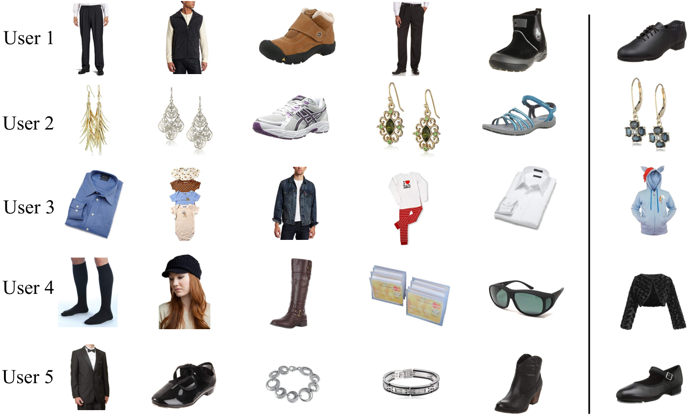
In this section, we list some failed examples of DIR-RNN and analyze the reason in detail. Figure 10 performs Five failed examples of DIR-RNN. Each row is a user’s purchase sequence. The predictions of DIR-RNN are listed on the right side. The failed examples mainly come from three reasons. First, DIR-RNN some times could not totally figure out preference changing from one attribute to another. For example, User1’s purchase history indicts that he prefers formal suits, so DIR-RNN recommends a leather shoes, while the user prefers casual shoes now. User2 always buys ear rings, but her preference changes to shoes recently. Second, some users’ purchase sequences are difficult to predict, such as User3 and User4. User3 may be a father. He buy things for his child and himself together. DIR-RNN confuses of his preference on categories. User4 tends to buy things of similar style. DIR-RNN recommends a jacket corresponding to the style, but she buy a pair of sunglasses which is also suitable. Third, DIR-RNN sometimes ignores the meticulous diversity of items. DIR-RNN recommends a pair of women’s leather shoes for User5, which appeal to her preference. As we can see in Figure 10, User5 has bought a similar pair of leather shoes before, so she chooses a pair of different ones. This difference could only be distinguished by image, which is not yet adopted in DIR-RNN.
5. Conclusion
In this paper, we have proposed a novel DIR to model attribute-level disentangled representations of items. The LearnDIR is further introduced to train the models under the framework of DIR. We apply DIR to two typical models as DIR-MF and DIR-RNN. Our experiments have shown that the DIR could establish an elaborate item representation for collaborative models, and the proposed model outperforms the state-of-the-art results. DIR allocates the items into tensor-like attribute embeddings, which has great benefits in reducing the parameter size and alleviating the cold-start problem. Besides, the only trade off comes from the complexity during training. Since additional training time does not have much influence in most real-world applications, DIR is workable.
In the future, first, we are going to take multimodal information like visual information into account, to enrich the representation. Second, we try to adapt the DIR to user representation. The code will soon be released 44 4 https://github.com/CRIPAC-DIG/DIR..
Acknowledgements.
This work is supported by National Key Research and Development Program (2018YFB1402605, 2018YFB1402600), National Natural Science Foundation of China (U19B2038, 61772528), Beijing National Natural Science Foundation (4182066).References
- (1)
- Ahuja (2017) Ravindra K Ahuja. 2017. Network flows: theory, algorithms, and applications. Pearson Education.
- Bao et al. (2019) Shilong Bao, Qianqian Xu, Ke Ma, Zhiyong Yang, Xiaochun Cao, and Qingming Huang. 2019. Collaborative Preference Embedding against Sparse Labels. In Proceedings of the 27th ACM International Conference on Multimedia. 2079–2087.
- Chen et al. (2016) Xi Chen, Yan Duan, Rein Houthooft, John Schulman, Ilya Sutskever, and Pieter Abbeel. 2016. Infogan: Interpretable representation learning by information maximizing generative adversarial nets. In Advances in neural information processing systems. 2172–2180.
- Cui et al. (2019) Qiang Cui, Shu Wu, Yan Huang, and Liang Wang. 2019. A hierarchical contextual attention-based network for sequential recommendation. Neurocomputing 358 (2019), 141–149.
- Gers et al. (2000) Felix A. Gers, Jürgen Schmidhuber, and Fred A. Cummins. 2000. Learning to Forget: Continual Prediction with LSTM. Neural Computation 12, 10 (2000), 2451–2471.
- He et al. (2016) Ruining He, Chunbin Lin, Jianguo Wang, and Julian McAuley. 2016. Sherlock: Sparse Hierarchical Embeddings for Visually-Aware One-Class Collaborative Filtering. In IJCAI. 3740–3746.
- He and McAuley (2016a) Ruining He and Julian McAuley. 2016a. Ups and downs: Modeling the visual evolution of fashion trends with one-class collaborative filtering. In WWW. 507–517.
- He and McAuley (2016b) Ruining He and Julian McAuley. 2016b. VBPR: Visual Bayesian Personalized Ranking from Implicit Feedback.. In AAAI. 144–150.
- Higgins et al. (2018) Irina Higgins, David Amos, David Pfau, Sebastien Racaniere, Loic Matthey, Danilo Rezende, and Alexander Lerchner. 2018. Towards a Definition of Disentangled Representations. arXiv preprint arXiv:1812.02230 (2018).
- Hochreiter and Schmidhuber (1997) Sepp Hochreiter and Jürgen Schmidhuber. 1997. Long short-term memory. Neural computation 9, 8 (1997), 1735–1780.
- Hou et al. (2019) Min Hou, Le Wu, Enhong Chen, Zhi Li, Vincent W Zheng, and Qi Liu. 2019. Explainable fashion recommendation: a semantic attribute region guided approach. arXiv preprint arXiv:1905.12862 (2019).
- Hu et al. (2019) Guangneng Hu, Yu Zhang, and Qiang Yang. 2019. Transfer Meets Hybrid: A Synthetic Approach for Cross-Domain Collaborative Filtering with Text. In The World Wide Web Conference. 2822–2829.
- John et al. (2018) Vineet John, Lili Mou, Hareesh Bahuleyan, and Olga Vechtomova. 2018. Disentangled Representation Learning for Text Style Transfer. arXiv preprint arXiv:1808.04339 (2018).
- Koren et al. (2009) Yehuda Koren, Robert Bell, and Chris Volinsky. 2009. Matrix factorization techniques for recommender systems. Computer 42, 8 (2009).
- Li et al. (2016) Xiang Li, Tao Qin, Jian Yang, Xiaolin Hu, and Tieyan Liu. 2016. LightRNN: Memory and Computation-Efficient Recurrent Neural Networks. In NIPS. 4385–4393.
- Lian et al. (2014) Defu Lian, Cong Zhao, Xing Xie, Guangzhong Sun, Enhong Chen, and Yong Rui. 2014. GeoMF: joint geographical modeling and matrix factorization for point-of-interest recommendation. In SIGKDD. 831–840.
- Liu et al. (2016b) Qiang Liu, Shu Wu, Diyi Wang, Zhaokang Li, and Liang Wang. 2016b. Context-aware sequential recommendation. In Data Mining (ICDM), 2016 IEEE 16th International Conference on. IEEE, 1053–1058.
- Liu et al. (2017) Qiang Liu, Shu Wu, and Liang Wang. 2017. DeepStyle: Learning User Preferences for Visual Recommendation. In SIGIR. 841–844.
- Liu et al. (2016a) Qiang Liu, Shu Wu, Liang Wang, and Tieniu Tan. 2016a. Predicting the Next Location: A Recurrent Model with Spatial and Temporal Contexts.. In AAAI. 194–200.
- Mathieu et al. (2016) Michael F Mathieu, Junbo Jake Zhao, Junbo Zhao, Aditya Ramesh, Pablo Sprechmann, and Yann LeCun. 2016. Disentangling factors of variation in deep representation using adversarial training. In Advances in Neural Information Processing Systems. 5040–5048.
- McAuley et al. (2015) Julian McAuley, Christopher Targett, Qinfeng Shi, and Anton Van Den Hengel. 2015. Image-based recommendations on styles and substitutes. In SIGIR. 43–52.
- McAuley and Leskovec (2013) Julian John McAuley and Jure Leskovec. 2013. From amateurs to connoisseurs: modeling the evolution of user expertise through online reviews. In Proceedings of the 22nd international conference on World Wide Web. 897–908.
- Mikolov et al. (2013a) Tomas Mikolov, Kai Chen, Greg Corrado, and Jeffrey Dean. 2013a. Efficient estimation of word representations in vector space. arXiv preprint arXiv:1301.3781 (2013).
- Mikolov et al. (2013b) Tomas Mikolov, Ilya Sutskever, Kai Chen, Greg S Corrado, and Jeff Dean. 2013b. Distributed representations of words and phrases and their compositionality. In NIPS. 3111–3119.
- Pan et al. (2008) Rong Pan, Yunhong Zhou, Bin Cao, Nathan N Liu, Rajan Lukose, Martin Scholz, and Qiang Yang. 2008. One-class collaborative filtering. In ICDM. IEEE, 502–511.
- Pennington et al. (2014) Jeffrey Pennington, Richard Socher, and Christopher D. Manning. 2014. GloVe: Global Vectors for Word Representation. In Empirical Methods in Natural Language Processing (EMNLP). 1532–1543. http://www.aclweb.org/anthology/D14-1162
- Rendle et al. (2009) Steffen Rendle, Christoph Freudenthaler, Zeno Gantner, and Lars Schmidt-Thieme. 2009. BPR: Bayesian Personalized Ranking from Implicit Feedback. In UAI, Proceedings of the Twenty-Fifth Conference on Uncertainty in Artificial Intelligence. 452–461.
- Rendle et al. (2010) Steffen Rendle, Christoph Freudenthaler, and Lars Schmidt-Thieme. 2010. Factorizing personalized markov chains for next-basket recommendation. In WWW. 811–820.
- Shin et al. (2019) Yong-Goo Shin, Yoon-Jae Yeo, Min-Cheol Sagong, Seo-Won Ji, and Sung-Jea Ko. 2019. Deep Fashion Recommendation System with Style Feature Decomposition. In 2019 IEEE 9th International Conference on Consumer Electronics (ICCE-Berlin). IEEE, 301–305.
- Sun et al. (2017a) Zhu Sun, Jie Yang, Jie Zhang, and Alessandro Bozzon. 2017a. Exploiting both Vertical and Horizontal Dimensions of Feature Hierarchy for Effective Recommendation.. In AAAI. 189–195.
- Sun et al. (2017b) Zhu Sun, Jie Yang, Jie Zhang, Alessandro Bozzon, Yu Chen, and Chi Xu. 2017b. MRLR: Multi-level Representation Learning for Personalized Ranking in Recommendation. In IJCAI. 2807–2813.
- Sundermeyer et al. (2012) Martin Sundermeyer, Ralf Schlüter, and Hermann Ney. 2012. LSTM Neural Networks for Language Modeling. In INTERSPEECH 13th Annual Conference of the International Speech Communication Association. 194–197.
- Yan et al. (2019) Cairong Yan, Yizhou Chen, and Lingjie Zhou. 2019. Differentiated fashion recommendation using knowledge graph and data augmentation. IEEE Access 7 (2019), 102239–102248.
- Yang et al. (2019) Xun Yang, Xiangnan He, Xiang Wang, Yunshan Ma, Fuli Feng, Meng Wang, and Tat-Seng Chua. 2019. Interpretable Fashion Matching with Rich Attributes. In Proceedings of the 42nd International ACM SIGIR Conference on Research and Development in Information Retrieval. 775–784.
- Yu et al. (2016) Feng Yu, Qiang Liu, Shu Wu, Liang Wang, and Tieniu Tan. 2016. A dynamic recurrent model for next basket recommendation. In SIGIR. 729–732.
- Yu et al. (2018) Wenhui Yu, Huidi Zhang, Xiangnan He, Xu Chen, Li Xiong, and Zheng Qin. 2018. Aesthetic-based clothing recommendation. In Proceedings of the 2018 World Wide Web Conference on World Wide Web. International World Wide Web Conferences Steering Committee, 649–658.
- Zhang et al. (2019) Shuai Zhang, Lina Yao, Aixin Sun, and Yi Tay. 2019. Deep learning based recommender system: A survey and new perspectives. ACM Computing Surveys (CSUR) 52, 1 (2019), 1–38.