Multiphase Circumnuclear Gas in a Low-$\beta$ Disk: Turbulence and Magnetic Field ReversalsJournal: ApJ

We study the pc-scale magnetized gas disk using 3D MHD simulations, considering radiative cooling and various heating effects in the cylindrical coordinate $(R,\varphi,z)$. The resistive MHD equations are:

where $\bm{B}$ is the magnetic field, $\rho$ is the gas density, $\rho\equiv m_{\rm H}n\sim m_{\rm H}(n_{n}+n_{i})$ with number densities of neutral and ionized hydrogen. $P_{\rm g}$ is the thermal gas pressure. The gas temperature is adopted as that of an ideal gas with the specific heat ratio $\gamma_{\rm g}=5/3$. The gravitational potential is assumed to be the Newtonian potential, $\Phi=GM_{\rm BH}/r$, where $G$ is the gravitational constant, $M_{\rm BH}=10^{7}M_{\sun}$ is the mass of the SMBH, and $r=\sqrt{R^{2}+z^{2}}$ is the distance from the SMBH. The electric field $\bm{E}$ obeys the Ohm’s law, $\bm{E}=-\bm{v}\times\bm{B}+\eta\bm{\nabla}\times\bm{B}$. We assume the anomalous resistivity $\eta$ as modeled by Yokoyama & Shibata 1994,

where $v_{d}=|\bm{\nabla}\times\bm{B}|/\rho$ is the electron-ion drift velocity, $v_{c}=10^{8}$ cm s^-1 is the critical velocity, and we adopted $\eta_{0}=10^{-9}$ and $\eta_{\rm max}=10^{-6}$ pc² yr^-1, respectively. Note that the results presented below are not sensitive to $\eta_{0}$ and $\eta_{\rm max}$ (see also, the Appendix A).

The radiative cooling and heating term $\rho{\cal L}$ in Equation 5 is given as

where the cooling function $\Lambda$ (Figure 1) is taken from Meijerink & Spaans 2005 and Wada et al. 2009. As a major heating source, we consider that X-ray photons come from the accretion disk, and the heating function is $\Gamma_{\rm X}=\Gamma_{\rm Coulomb}+\Gamma_{\rm Compton}+\Gamma_{\rm photoionic}$. The Coulomb interaction is given by

where $\eta_{\rm h}$ is the efficiency in fixed $0.2$, and $H_{\rm X}$ is the X-ray energy deposition rate, $H_{\rm X}=3.8\times 10^{-25}\xi{\rm~erg~s}^{-1}$. For the Compton and photoionization interactions, we use a formula given by Blondin 1994, i.e.

where $T_{\rm X}=10^{8}$ K is the characteristic temperature of an X-ray photon. Here the ionization parameter $\xi$ is

where $L_{\rm X}$ is X-ray luminosity and $L_{\rm Edd}$ is the Eddington luminosity for $M_{\rm BH}=10^{7}M_{\sun}$. In this simulation, we set $\xi=100$ for simplicity.

The photoelectric heating, assuming spatially uniform FUV is taken into account,

We start the simulation from an equilibrium torus. In order to construct the equilibrium torus solutions with a toroidal field, we assume the polytropic relation,

where $K$ is the polytropic constant, and the weak toroidal field $B_{\varphi}$ is given by plasma-$\beta$, $\beta=100$. To give the density distribution, we assume the rotation velocity to be the radial distribution of angular momentum $L(R)$,

where $L_{0}(\equiv R_{0}v_{0})$ and $R_{0}$ adopt the normalized units and $a=0.35$ is the power index. The flux surface $\Psi(R,z)$ is then given as

where $c_{s}^{2}=\gamma_{\rm g}P_{\rm g}/\rho$ is the square of the sound speed and $v_{A}^{2}=B_{\varphi}^{2}/(4\pi\rho)$ is the square of the Alfvén speed. We defined the normalized unit as the torus density maximum, $\Psi_{0}=\Psi(R_{0},0)$. For the condition of positive pressure, we can obtain a torus density distribution $\Psi(R,z)=\Psi_{0}$,

We assume that the torus is embedded in the isothermal nonrotating and nonmagnetized halo, with pressure and density given by

The normalized quantities are listed in Table 1. The polytropic indexes $K$ and $K_{\rm h}$ are parameterized by the square of the velocity ratio, $\varepsilon=K\rho_{0}^{\gamma_{\rm g}-1}/v_{0}^{2}=\gamma_{\rm g}^{-1}c_{s}^{2}(R_{0},0)/v_{0}^{2}$ in the normalization, and we set $\varepsilon=0.04$ in the torus and $\varepsilon_{\rm h}=2$ in the halo, respectively.

We use CANS+ code (Matsumoto et al. 2019), which is implemented using the HLLD solver (Miyoshi & Kusano 2005, Harten-Lax-van Leer discontinuitues;) with div $B$ cleaning (Dedner et al. 2002) and three-stage total variation diminishing Runge-Kutta time integration (TVDRK). The fifth-order accuracy in space is achieved through the Monotonicity Preserving method (Suresh & Huynh 1997, MP5;) to capture small-scale magnetic fluctuations. Basic equations are solved using conservative forms with geometrical and gravitational source terms explicitly included. After TVDRK updating, the cooling and heating source terms are treated in the implicit operator splitting approach.

As a numerical constraint in our simulation, we set the floor of the gas pressure in the grid cells where the minimum temperature is $T=20$ K or the minimum plasma-$\beta$ is $\beta=0.001$. Comparing the volume-averaged energies of the grid cells where the lower limit is applied, the thermal energy is always 2-3 orders of magnitude smaller than the kinetic and magnetic energies. This implies that the artificial thermal energy due to the numerical floor does not affect the gas dynamics.

The size of the simulation box is $0\leq R/R_{0}<12$, $0<\varphi$ [rad]$<2\pi$, $|z/R_{0}|<3$. The grid size is $\Delta R=0.01R_{0}$ and $\Delta z=0.002R_{0}$. We use a coarser grid size outside for $R/R_{0}>2.0$ or $|z/R_{0}|>0.4$, and for the region around the axis $R/R_{0}<0.2$. The numbers of grid cells are $N_{R}=256$, $N_{\varphi}=512$, and $N_{z}=512$.

We assume the outflow boundary condition for the outer boundaries (i.e. $R/R_{0}=10$ and $|z|/R_{0}>2.8$). For the azimuthal direction, the periodic boundary condition is assumed. Meshes around the cylindrical axis are sent to the opposite computational domain of the azimuthal direction, which means that fluid can flow across the polar axis ($R=0$). In the central region for $r/R_{0}<0.4$, we impose an absorbing boundary condition, i.e.

where $q$ and $q_{\rm init}$ are the primitive variables of the TVDRK updating state and the initial state, respectively. Damping function $D(r)$ is modeled as,

We start the simulations assuming the adiabatic MHD, then after the magnetic field strength sufficiently develops and the system becomes a quasi-steady state at $t\leq 0.477$ Myr (25 rotational periods at $R=1$ pc), the cooling and heating terms are considered until $t\leq 3.64$ Myr (97 rotational periods).

Figure 2 shows three snapshots ($t=0.000,0.744$ and 2.353 Myr) of the gas temperature and the plasma-$\beta$ on a $R$-$z$ plane. Figure 2a shows the initial conditions. As explained in Section II.3, the system evolves adiabatically until $t=0.477$ Myr. During this period, gas spreads out vertically, and intense magnetic field fluctuations are developed by the MRI and $\beta>0.6$ inside the torus. The magnetic field is stronger near the surface of the torus with $\beta\sim 0.2$. MRI causes not only turbulent motion but also heating due to magnetic reconnection. After cooling and heating are taken into account, the structure of the torus changes (Figure 2c). The plasma-$\beta$ around the midplane becomes smaller with $0.003<\beta<6.0$. The torus becomes geometrically thinner, and it consists of two components: cold disk ($T\lesssim 10^{3}$ K) and warm disk ($T=10^{3-5}$ K). The cold, thin disk ($R<2$ pc) is supported vertically by the magnetic field as discussed below.

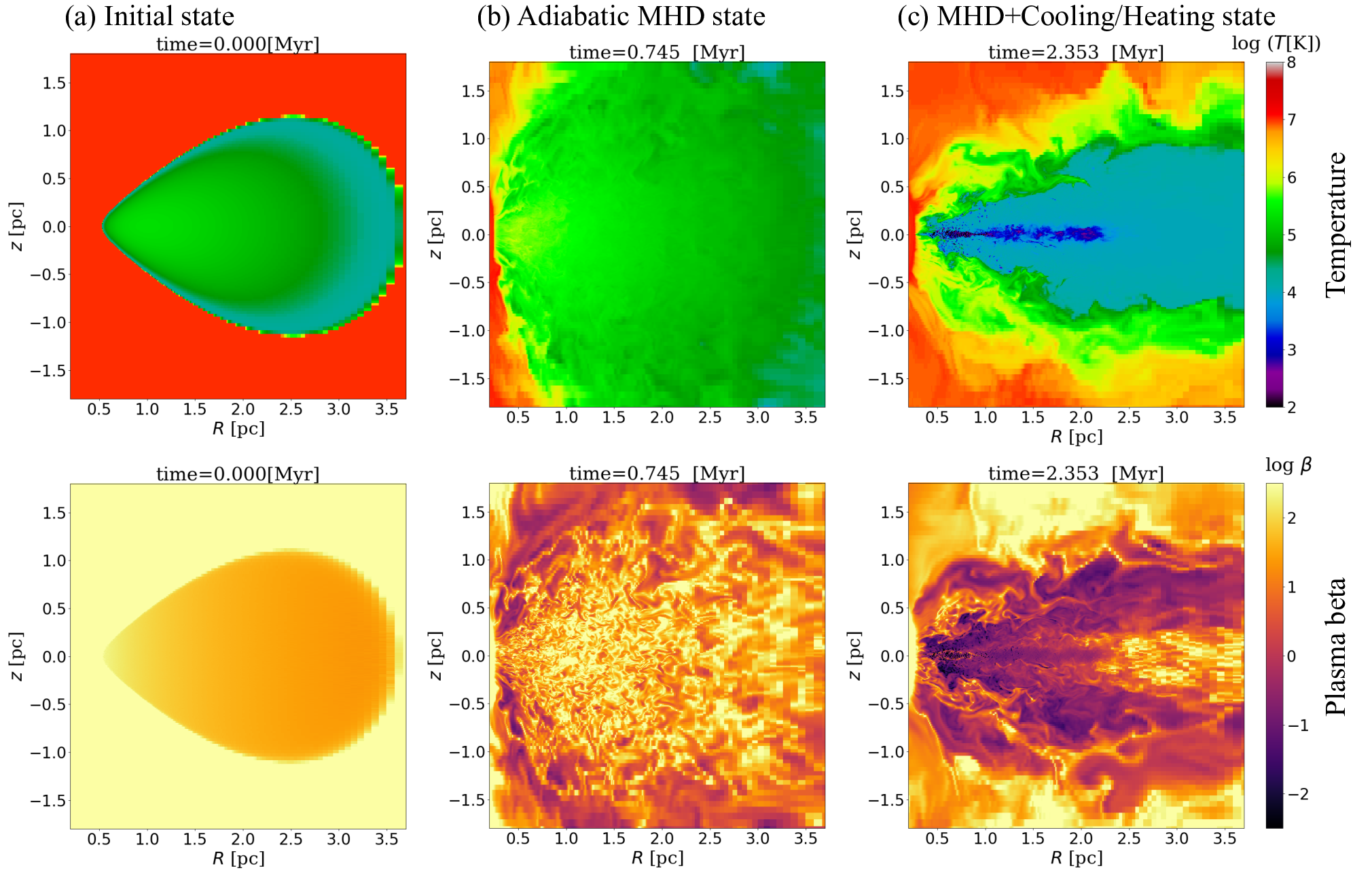
Figure 3 shows the magnetic field structure at $t=0.744$ Myr of the adiabatic MHD state. The turbulent field in the torus dominates in the $R$-$z$ and $R$-$\varphi$ planes. The toroidal field ($B_{\varphi}$) shows the flux bundle of the positive direction (red) around the torus surface at $|z|=1.5$ pc.

Figure 4 is the same as Figure 3, but cooling and heating are considered ($t=2.353$ Myr). The field strength and turbulent fluctuation are markedly different from those in Figure 3. The toroidal field $B_{\varphi}$ dominates the total magnetic field. The two plots of $B_{\varphi}$ show that the mean toroidal field has more coherent structures compared to the that in the adiabatic phase (Figure 3) with opposite directions shown in blue and red in Figure 4. On the other hand, radial and vertical magnetic fields are dominated by the turbulent component. We can also see that the patches of $B_{R}$ and $B_{z}$ with opposite directions tend to extend radially and vertically, respectively.

For a more quantitative observation, we decomposed the magnetic energy into mean and turbulent components. We measured the mean component as the azimuthal average,

Hence, the turbulent component is derived as,

where we notate the mean as $\bar{~}$ and the turbulence as $\delta$. Figure 5 shows the evolution of the magnetic energy in each component. It is clear that the structures of the magnetic field change drastically after the cooling and heating. For $t<0.5$ Myr, turbulent fields become exponentially stronger than mean fields, while the ratios between them are approximately constant, i.e. $\delta B_{\varphi}^{2}/\delta B_{R}^{2}\sim 10$ and $\delta B_{\varphi}^{2}/\delta B_{z}^{2}\sim 22$. After cooling/heating at $t=0.744$ Myr, the turbulent fields decrease quickly by one order of magnitude, and they survive until $t\sim 3.5$ Myr. This turbulent field dissipation is caused by the decrease in the gas temperature (see in Section IV). During this phase, we found that $|\delta B_{\varphi}|>|\delta B_{R}|>|\delta B_{z}|$, but the ratios between them change.

In the adiabatic MHD state, the amplitude of $\overline{B}_{\varphi}$ (blue solid line in Figure 5) reaches a quasi-steady state with a periodical cycle of $T_{\rm cycle}=0.163$ Myr $\sim 9.1$ rotational periods. After cooling/heating effects are included, oscillating amplification of $\overline{B_{\varphi}}$ continues for $0.744<t<1.75$ Myr. The quasi-steady state is achieved when $\overline{B_{\varphi}}$ does not significantly change . However, $|\overline{B_{\varphi}}|$ shows quasi-periodic oscillations on a long time scale beyond reaching steady state. This amplitude and period become larger and longer than those of the adiabatic MHD state. Around the maximum of $|\overline{B_{\varphi}}|$ (i.e. $t=1.75,3.08$ Myr), $|\delta\bm{B}|$ and $|\overline{B_{R}}|$ are maximized, and around the minimum of that (i.e. $t=2.1,3.2$ Myr), $|\delta\bm{B}|$ and $|\overline{B_{R}}|$ are maximized. We show the quasi-periodic spatial changing in the animation of Figure 4.

Steady-state behavior is also seen from examining the mass flux inside 0.9 pc for $t>1.75$ Myr. The radial profile of the net mass accretion rate appears to be roughly constant in time, which has been observed in simulation studies (Stone & Pringle 2001; Jiang et al. 2019, e.g.). We took the time averages over 1.6 Myr, which is the longest time scale in the periodic oscillation of $|\overline{B_{\varphi}}|$. The time variation of the mass accretion rate due to MRI turbulence has been discussed in O’Neill et al. 2011, Hawley et al. 2011, and Hogg & Reynolds 2016. Since the mass flux varies with the averaging time interval, the time domain $0.744<t<1.75$ Myr is not steady.

The periodical cycle of the mean toroidal field energy is observed to have the pattern of a quasi-periodic direction reversal. Figure 6 (top), the so-called the butterfly diagram, is the space ($z$-direction) time evolution of the mean toroidal field direction at $R=0.715$ pc. It shows that the direction periodically changes at a given $z$, and it also implies that the $B$-field escapes from the midplane. Figure 6 (bottom) is for the mean plasma-$\beta$, $\overline{\beta}\equiv 2\overline{P_{\rm g}}/\overline{|\bm{B}|^{2}}$. The disk surface traces the bounding surface for $\overline{\beta}\leq 10$. This implies that the magnetic field becomes amplified near the midplane and is transferred to the high latitudes of the disk. The quasi-steady radial mass flow indicates the saturation of the MRI-driven turbulence.

In the MHD+cooling/heating state ($t>0.744$ Myr), the lowest plasma-$\beta$ is in the midplane, and mean field transport is slower than that of the adiabatic MHD. The direction of $B_{\varphi}$ in $1.20<t$ Myr $<2.27$ is vertically stratified in blue around the mid-plane and red above that. The vertical transport changes from slow to fast at time $t=1.74$ Myr. Recall that the energy of $B_{\varphi}$ increases and decreases in Figure 5, and this time is the maximum point. The same phenomenon occurs on the next reversal where it is red around the midplane and blue above that. We have confirmed the cycle through the mean toroidal field direction reversal and escape from the disk.

The vertical escape of the mean field is described as the vertical magnetic energy transport using the Poynting flux $F_{P,~z}$,

where a rise speed $v_{B}$ denotes the vertical derivative of the pattern of the mean toroidal field (Salvesen et al. 2016b). The large rise speeds occur at the direction reversal, and large fall speeds appear around the midplane and $|z|>0.5$ pc (Figure 7). The maximum rise speed $v_{B}$ is 37.3 km s^-1 in $|z|<0.8$ pc. In the same way, Alfvén speed and vertical speed are measured as $|\bm{v}_{A}|\sim 41.6$ km s^-1 and $|v_{z}|\sim 44.0$ km s^-1, and these speeds are comparable. The rise speed cannot reach the gravitational escape speed, $244.8$ km s^-1 at $R=0.715$ pc.

In this subsection, we investigate the physical origin of the turbulent magnetic field shown in Section III.1 and how it is maintained. Figure 8 shows the turbulent velocity field of the gas at $t=2.353$ Myr. The maximum upflow (blue arrows) is about 18$\%$ of the escape velocity at that position. The gas circulates with downward and upward flows in the ambient, where $\log\left\{P_{\rm g}/(\gamma_{\rm g}-1)\right\}\lesssim-4$. The velocity inside the disk is relatively smaller than that in the ambient. The magnitude of the turbulent velocity for $R\lesssim 0.9$ pc is comparable to the sound speed. That for $R\gtrsim 0.9$ pc is roughly 10$\%$ of the sound speed. The direction of vectors does not coincide with the turbulent and mean magnetic fields; however, part of the gas falls into the midplane along the magnetic field lines. Each component of the turbulent field and velocity has a difference only within one order of magnitude.

Figure 9 shows the vertical structures of the magnetic, thermal, and kinetic energies at a given radius at $t=2.533$ Myr. Around the midplane, the mean toroidal magnetic field dominates the turbulent magnetic and kinetic energies ($\overline{\rho}\overline{|\delta\bm{v}|^{2}}/2$), both of which are comparable to the thermal energy ($\overline{P_{\rm g}}/(\gamma_{\rm g}-1)$). The mean field decreases more rapidly than the turbulent component with $z$. As a result, there are regions where $\overline{\delta B_{\varphi}^{2}}>\overline{B}_{\varphi}^{2}$ ($0.2\lesssim|z|$ pc $\lesssim 0.8$). The transition between the turbulent component and the mean field also occurs at the disk surface ($|z|\sim 0.05$ pc), where the mean field reverses its direction as seen in Figure 6. At higher latitude ($|z|\gtrsim 0.3$ pc), contrary to the midplane ($z=0$ pc), turbulent toroidal field energy ($\overline{\delta B_{\varphi}^{2}}/2$) is about 10 $\%$ of the mean thermal energy, but it is comparable to or a few times larger than the kinetic energy.

The vertical random motion could be related to the magnetoconvective instability (or interchange instability, see, e.g., Acheson 1979). The unstable criterion is

This criterion corresponds to the convective instability for the gas with decreasing specific entropy $s$ with large $|z|$, i.e.

Replacing $P_{\rm g}$ and $\gamma_{\rm g}$ in the relation (27) with $P_{B}$ and $\gamma_{B}$, where the magnetic pressure $P_{B}=|\bm{B}|^{2}/2$, the criterion (26) is obtained. Here $\gamma_{B}=1+P_{B}/U_{B}=2$ for the energy density $U_{B}=|\bm{B}|^{2}/2$ (Kulsrud 2005, e.g.,). The criterion (26) can be written as $d\left(|B_{\varphi}|/\rho\right)/dz<0$. Therefore, the instability occurs when the mass frozen in the magnetic flux tube per unit length increases with increasing $|z|$.

One should note that the criteria (27) and (26) are necessary conditions for convection. We compare the two criteria with the vertical variation of the modified plasma $\hat{\beta}$, i.e. $\hat{\beta}\equiv\left(\overline{P_{\rm g}}+\overline{P_{\rm K}}\right)/\overline{P_{B}}$ in Figure 10, where ${P_{\rm K}}\equiv\overline{\rho}\delta{\bm{v}}^{2}$. Note that the strong ram pressure exists around the midplane, and $P_{\rm K}\sim P_{\rm g}$, but magnetic energy dominates. In the bottom panel of Figure 10, hydrodynamic convection is essentially stable, i.e. the positive entropy gradient shown in shadows in red shadows. In contrast, as seen in the top panel of Figure 10, there are many unstable regions for the magnetoconvective instability (blue shadows). From the conditions, i.e. $\frac{d}{dz}\left(\frac{P_{B}}{\rho^{2}}\right)<0$(unstable), $\frac{d}{dz}\left(\frac{P_{\rm g}}{\rho^{\gamma_{\rm g}}}\right)>0$ (stable), after some algebraic calculations to vanish the density gradient, we can derive

When $d|B_{\varphi}|/dz\sim 0$ (i.e. when field direction reversal occurs) and/or $\gamma_{\rm g}/2\sim 1$, this condition satisfies $d\beta/dz>0$. Figure 10 shows that the regions with $d\hat{\beta}/dz>0$ correspond to unstable regions for magnetoconvective instability.

The two panels of Figure 11 show the unstable regions for the two criteria, (26) and (27). They show that the unstable regions for the magnetoconvection form belt-like layers, where the mean toroidal field direction reverses (see, $B_{\varphi}$ on the $R$-$z$ plane in Figure 4). The unstable layers move with the rising direction pattern of the mean toroidal field. The width of the unstable layers remains approximately constant around $0.05$-$0.1$ pc. The bottom panel implies that the system is convectively stable.

Figure 12 shows the vertical distributions of the density and temperature at $R=0.715$ pc at $t=2.353$ Myr. For $|z|<0.05$ pc, the gas is cold ($\sim 8\times 10^{2}$ K) and dense ($n\sim 10^{3}$ cm^-3). As seen in Figure 2(c), this cold disk extends to $R\sim 2$ pc. Outside this cold, dense disk, the gas is warm ($\sim 10^{4}$ K) and less dense ($n\sim 10$ cm^-3); therefore, they are roughly in pressure equilibrium. The temperature of the ambient region ($|z|>0.25$ pc) increases continuously until $\sim 10^{6}$ K. Figure 12 also shows that there is a large azimuthal fluctuation around the mean values. The density fluctuation is in the order of unity or less while the temperature, as a maximum, fluctuates by three orders of magnitude. For the cold disk ($|z|<0.05$ pc), the minimum temperature reaches the lower limit, and the maximum does not exceed $10^{4}$ K of the warm disk.

To quantify the temperature and density fluctuations in phase space, we plot the gas mass fraction as a function of gas pressure and number density in the top panel of Figure 13. A large amount of gas mass is collected in characteristic regions over the gas mass fraction $\log(M/M_{\rm tot})>-5$. These are multiphase states created by the thermal instability. The gas is also distributed in a wide range of densities and temperatures, but a large fraction of the gas is in a state with $P_{\rm g}/k_{B}\gtrsim 10^{5}$ and $n\gtrsim 1$. The bottom panel in Figure 13 shows the spatial distributions of four thermal states shown in the top panel on the $R$-$z$ plane. The colors represent the region enclosed by the same colors on $P_{\rm g}$-$n$ plane. The low-temperature gases is patchy in the warm ($\sim 10^{4}$ K) thick disk shown in blue. The mass fraction of this low-temperature gas is small. Although the mass fraction of gas in the red region is small, The green region refers to the dense gas in a cold ($\sim 100$ K) phase. The gas shown in yellow in the top panel mostly forms the thick disk at $R>0.9$ pc as shown in the bottom panel, where they are approximately isothermal (therefore, the gas pressure is constant).

In Figure 14, density and temperature for $R<0.9$ pc (i.e., the quasi-steady cold, thin gas disk) are plotted as a functions of the magnetic pressure $P_{\rm B}$ and the thermal pressure $P_{\rm g}$ at $t=2.35$ Myr. In the region where magnetic pressure dominates ($\beta<1$), the number density of the left panel is distributed in a wide range from $n\sim 10^{-2}$ to $10^{4}$ cm^-3 for a given gas pressure. It shows that the temperature is lower than $T\sim 10^{5}$ K, and the strongly magnetized gas consists of cold gas with $T<1000$ K, which dominates the total mass (Figure 13). In the high-$\beta$ domain, the temperature and density fixed at gas pressure are not sensitive to changes in magnetic field. The thermal state is determined by the compression and expansion of the gas pressure.

In the above results, we observe a thin cold ($T<100$ K) disk where the magnetic field is strong ($\beta\lesssim 1$) at $R<0.9$ pc (see Figures 13 and 14). This structure is stable at least until the end of the simulation, i.e. $t\sim 3.6$ Myr ( $\sim 96$ rotational periods at $R=1$ pc). The disk is maintained by the MRI and by the mass inflow from the outer disk ($R>0.9$ pc), where the gas is less dense and less magnetized. Therefore, we suspect that this strongly magnetized disk is not “transient”, and it could last during the lifetime of the AGNs ($\sim 10$ Myr).

If this is the case, a strong magnetic field at $R<1$ pc could be expected in AGNs, and it can be observable by the Zeeman effect using future observations by ALMA, ng-VLA, and SKA.

If the mass supply from the outer region is stopped, the magnetic field can be dissipated by the ambipolar diffusion (see, Equation A10 and the Appendix A). The expected time scale is

which is still long enough to be observed.

We found that the low-$\beta$ disk formed by radiative cooling and heating is discernible by the direction reversal (Fig. 6) and vertical transfer of the magnetic field (Fig. 7). A long reversal period is observed in the strong toroidal field with low-$\beta$ compared to the turbulence with high-$\beta$. This trend is also found in the local 3D simulations of an isothermal gas (Bai & Stone 2013; Salvesen et al. 2016b). The mean plasma-$\beta$, $\overline{\beta}\sim 0.1-0.4$ in the midplane is also similar to our result (Salvesen et al. 2016b, see, Fig. 10; Table 2 of). Compared to an analytical model (Begelman et al. 2015), it was demonstrated that heating efficiency, defined as the ratio between the dissipation rate (e.g. the magnetic reconnection) and mean toroidal field production rate, decreases with $\beta$. Salvesen et al. 2016b showed that assuming steady Poynting flux, the period of the direction reversal is proportional to the rotational period ($T_{\rm cycle}=2\pi/\Omega\xi_{B}^{-1}$) and is determined by the phenomenological parameters; $\xi_{B}=\nu\eta_{B}/(\beta-\nu+1)$, where $v_{B}=\eta_{B}\Omega z$ (see also Equation 25) and $\nu$ is the degree of turbulent heating. The turbulent heating caused by the nonlinear MRI is weakened by the small plasma-$\beta$ (Salvesen et al. 2016b, see, Table 3 of).

The field direction reversal as seen in Figure 6 is caused by the changes in balance between the turbulent energy and the mean field energy. When the direction of the mean field, which is represented by two shaded colors, reverses (e.g., $t=1.20,2.12,3.48$ Myr in Figure 15), the energy density $\overline{B}_{\varphi}^{2}/2$ (blue solid line) temporarily drops and the turbulent magnetic field ($\delta\bm{B}_{\varphi}^{2}/2$; blue dotted line) is amplified. While the turbulent kinetic energy ($\overline{\rho}\delta\bm{v}^{2}/2$; black dotted line) exceeds the thermal energy ($\sim P_{\rm g}$; green solid line), the turbulent magnetic energy (blue dotted line) is smaller than the thermal energy of cold gas ($T\sim 1000$ K), i.e. $\beta$ at this moment becomes large. The direction reversal is caused by a combination of MRI and the Parker instability (Machida et al. 2013, Figure 16 or see, e.g.,). A magnetic field line with a small radial fluctuation (panel (a)) is stretched to the radial and azimuthal directions (panel (b)). The stretched field line with a longer wavelength is selectively buoyed up toward higher latitudes by the Parker instability (panel (c)). As a result, for the $R$-$\varphi$ plane, the buoyant field line has an opposite direction to the field line in the midplane. In the low-$\beta$ disk, direction reversal is possible by driving turbulence from the mean field; thus, the process to high $\beta$ will be important (i.e. magnetoconvection in Section III.3). Direction reversal was widely observed in adiabatic MHD simulations (Beckwith et al. 2011; O’Neill et al. 2011; Flock et al. 2012; Machida et al. 2013; Parkin & Bicknell 2013; Hogg & Reynolds 2016, e.g., ), but we found here for the first time that direction reversal also occurs in the low-$\beta$ disk with the multiphase gas ($10<T$ [K]$<10^{5}$).

We observed the strongly magnetized disk driven by MRI in Section 3. We discuss here what constrains the strength of the magnetic field (plasma-$\beta$) in this simulation. In Figure 10, the mean plasma-$\beta$ around the cold disk shows $\bar{\beta}>0.1$. This satisfies the condition for the MRI, i.e. $\bar{\beta}>\beta_{\rm crit}$ (Begelman & Pringle 2007), above which the MRI can be driven, and

where we adopted the Keplerian rotation $v_{K}$ at $R=0.715$ pc and the mean temperature in Figure 12. On the other hand, the mean plasma-beta is expressed as $\bar{\beta}^{-1}\sim(\delta B_{\varphi}^{2}/2+\overline{B_{\varphi}}^{2}/2)/P_{\rm g}$. For $\overline{B_{\varphi}}^{2}\geq\delta B_{\varphi}^{2}$, which is the case in the disk, $\bar{\beta}\leq P_{\rm g}/\delta B_{\varphi}^{2}$. From Figure 15, $P_{\rm g}/\delta B_{\varphi}^{2}\sim 10$, therefore, the mean plasma-beta can be constrained as $0.01\lesssim\bar{\beta}\lesssim 10$.

It has been known that the MRI-driven turbulence depends on numerical spatial resolution. Hawley et al. 2011; Hawley et al. 2013 applied the quality factor $Q_{\varphi}\equiv\lambda/(R\Delta\varphi)$, which is the resolution of the characteristic MRI wavelength ($\lambda=2\pi B_{\varphi}/\sqrt{\rho\Omega^{2}}$). They identified the empirical condition as $Q_{\varphi}\gtrsim 20$. However, for the toroidal field, the numerical convergence of adiabatic turbulence has not been clarified yet. The low-$\beta$ MRI in cold gas requires high resolution,

where $N_{\varphi}=2\pi/\Delta\varphi$ is the azimuthal resolution. In our model, $N_{\varphi}=512$ and we found that $Q_{\varphi}\gtrsim 20$ (Kudoh & Wada 2018, see, e.g.). Additionally, a comparison with $N_{\varphi}=128$ showed that the low resolution is $Q_{\varphi}<10$, and thus, there is no direction reversal in the cold and low-$\beta$ disk. Our simulations are in agreement with the estimation of Equation 31 and the empirical condition. In the long-term calculation, the turbulent magnetic field is sensitive to the numerical flux solver and the high-order accuracy. In order to reduce numerical dissipation, HLLD flux solver is employed (Hawley et al. 2013, see, e.g.). Matsumoto et al. 2019 pointed out that the high-order accuracy prevents the dissipation rather than the low-order scheme. We took a highly precise numerical approach, hence the differences from previous global 3D simulations.

AGNs emit enormous energy fluxes over a wide wavelength, and its feedback is important for the dynamics of the circumnuclear gas (Chan & Krolik 2016; Chan & Krolik 2017, e.g.,). However, IR radiative pressure is not dynamically effective (Namekata & Umemura 2016), and cannot contribute to MRI in the cold gas. Notably, the anisotropic radiation pressure on the dust in the gas with the X-ray heating produces flows in a fountain-like manner in the central tens-of-parsec pc regions around the AGNs (Wada 2012). The radiation pressure is expected to be stronger than the magnetic pressure, i.e.

where $\kappa_{d}=10^{5}$ is the dust opacity and $\alpha_{d}=0.01$ is the gas to dust ratio (Wada 2012). In a subsequent paper, we will investigate the effect of radiation pressure, how magnetic structures are changed, and how magnetic buoyancy or magnetoconvection can help.

References

- Acheson (1979) Acheson, D. J. 1979, Sol. Phys., 62, 23, doi: 10.1007/BF00150129
- Bai & Stone (2013) Bai, X.-N., & Stone, J. M. 2013, ApJ, 767, 30, doi: 10.1088/0004-637X/767/1/30
- Balbus & Hawley (1991) Balbus, S. A., & Hawley, J. F. 1991, ApJ, 376, 214, doi: 10.1086/170270
- Beckwith et al. (2011) Beckwith, K., Armitage, P. J., & Simon, J. B. 2011, MNRAS, 416, 361, doi: 10.1111/j.1365-2966.2011.19043.x
- Begelman et al. (2015) Begelman, M. C., Armitage, P. J., & Reynolds, C. S. 2015, ApJ, 809, 118, doi: 10.1088/0004-637X/809/2/118
- Begelman & Pringle (2007) Begelman, M. C., & Pringle, J. E. 2007, Monthly Notices of the Royal Astronomical Society, 375, 1070, doi: 10.1111/j.1365-2966.2006.11372.x
- Blondin (1994) Blondin, J. M. 1994, ApJ, 435, 756, doi: 10.1086/174853
- Braginskii (1965) Braginskii, S. I. 1965, Reviews of Plasma Physics, 1, 205. http://adsabs.harvard.edu/abs/1965RvPP....1..205B
- Chan & Krolik (2016) Chan, C.-H., & Krolik, J. H. 2016, ApJ, 825, 67, doi: 10.3847/0004-637X/825/1/67
- Chan & Krolik (2017) —. 2017, ApJ, 843, 58, doi: 10.3847/1538-4357/aa76e4
- Crocker et al. (2010) Crocker, R. M., Jones, D. I., Melia, F., Ott, J., & Protheroe, R. J. 2010, Nature, 463, 65, doi: 10.1038/nature08635
- Dedner et al. (2002) Dedner, A., Kemm, F., Kröner, D., et al. 2002, Journal of Computational Physics, 175, 645, doi: 10.1006/jcph.2001.6961
- Dorodnitsyn & Kallman (2017) Dorodnitsyn, A., & Kallman, T. 2017, ApJ, 842, 43, doi: 10.3847/1538-4357/aa7264
- Draine et al. (1983) Draine, B. T., Roberge, W. G., & Dalgarno, A. 1983, ApJ, 264, 485, doi: 10.1086/160617
- Ferrière (2009) Ferrière, K. 2009, A&A, 505, 1183, doi: 10.1051/0004-6361/200912617
- Flock et al. (2012) Flock, M., Dzyurkevich, N., Klahr, H., Turner, N., & Henning, T. 2012, ApJ, 744, 144, doi: 10.1088/0004-637X/744/2/144
- Fragile & Sa̧dowski (2017) Fragile, P. C., & Sa̧dowski, A. 2017, MNRAS, 467, 1838, doi: 10.1093/mnras/stx274
- Han (2017) Han, J. L. 2017, ARA&A, 55, 111, doi: 10.1146/annurev-astro-091916-055221
- Hawley et al. (2011) Hawley, J. F., Guan, X., & Krolik, J. H. 2011, ApJ, 738, 84, doi: 10.1088/0004-637X/738/1/84
- Hawley et al. (2013) Hawley, J. F., Richers, S. A., Guan, X., & Krolik, J. H. 2013, ApJ, 772, 102, doi: 10.1088/0004-637X/772/2/102
- Hogg & Reynolds (2016) Hogg, J. D., & Reynolds, C. S. 2016, ApJ, 826, 40, doi: 10.3847/0004-637X/826/1/40
- Hsieh et al. (2018) Hsieh, P.-Y., Koch, P. M., Kim, W.-T., et al. 2018, The Astrophysical Journal, 862, 150, doi: 10.3847/1538-4357/aacb27
- Izumi et al. (2018) Izumi, T., Wada, K., Fukushige, R., Hamamura, S., & Kohno, K. 2018, ApJ, 867, 48, doi: 10.3847/1538-4357/aae20b
- Jiang et al. (2019) Jiang, Y.-F., Stone, J. M., & Davis, S. W. 2019, The Astrophysical Journal, 880, 67, doi: 10.3847/1538-4357/ab29ff
- Kudoh & Wada (2018) Kudoh, Y., & Wada, K. 2018, Galaxies, 6, 139, doi: 10.3390/galaxies6040139
- Kulsrud (2005) Kulsrud, R. M. 2005, Plasma physics for astrophysics. https://ui.adsabs.harvard.edu/abs/2005ppfa.book.....K
- Liu et al. (2013) Liu, H. B., Ho, P. T. P., Wright, M. C. H., et al. 2013, ApJ, 770, 44, doi: 10.1088/0004-637X/770/1/44
- Lopez-Rodriguez et al. (2015) Lopez-Rodriguez, E., Packham, C., Jones, T. J., et al. 2015, MNRAS, 452, 1902, doi: 10.1093/mnras/stv1410
- Machida et al. (2013) Machida, M., Nakamura, K. E., Kudoh, T., et al. 2013, ApJ, 764, 81, doi: 10.1088/0004-637X/764/1/81
- Machida et al. (2009) Machida, M., Matsumoto, R., Nozawak, S., et al. 2009, PASJ, 61, 411, doi: 10.1093/pasj/61.3.411
- Matsumoto et al. (2019) Matsumoto, Y., Asahina, Y., Kudoh, Y., et al. 2019, PASJ, 71, 83, doi: 10.1093/pasj/psz064
- Meijerink & Spaans (2005) Meijerink, R., & Spaans, M. 2005, A&A, 436, 397, doi: 10.1051/0004-6361:20042398
- Mishra & Simon (2020) Mishra, B., B. M. C. A. P. J., & Simon, J. B. 2020, MNRAS, 492, 1855, doi: 10.1093/mnras/stz3572
- Miyoshi & Kusano (2005) Miyoshi, T., & Kusano, K. 2005, Journal of Computational Physics, 208, 315, doi: 10.1016/j.jcp.2005.02.017
- Modjaz et al. (2005) Modjaz, M., Moran, J. M., Kondratko, P. T., & Greenhill, L. J. 2005, ApJ, 626, 104, doi: 10.1086/429559
- Namekata & Umemura (2016) Namekata, D., & Umemura, M. 2016, MNRAS, 460, 980, doi: 10.1093/mnras/stw862
- Netzer (2015) Netzer, H. 2015, ARA&A, 53, 365, doi: 10.1146/annurev-astro-082214-122302
- Nishiyama et al. (2010) Nishiyama, S., Hatano, H., Tamura, M., et al. 2010, ApJ, 722, L23, doi: 10.1088/2041-8205/722/1/L23
- Nishiyama et al. (2013) Nishiyama, S., Yasui, K., Nagata, T., et al. 2013, ApJ, 769, L28, doi: 10.1088/2041-8205/769/2/L28
- O’Neill et al. (2011) O’Neill, S. M., Reynolds, C. S., Miller, M. C., & Sorathia, K. A. 2011, ApJ, 736, 107, doi: 10.1088/0004-637X/736/2/107
- Parkin & Bicknell (2013) Parkin, E. R., & Bicknell, G. V. 2013, ApJ, 763, 99, doi: 10.1088/0004-637X/763/2/99
- Salvesen et al. (2016a) Salvesen, G., Armitage, P. J., Simon, J. B., & Begelman, M. C. 2016a, MNRAS, 460, 3488, doi: 10.1093/mnras/stw1231
- Salvesen et al. (2016b) Salvesen, G., Simon, J. B., Armitage, P. J., & Begelman, M. C. 2016b, MNRAS, 457, 857, doi: 10.1093/mnras/stw029
- Spitzer (1962) Spitzer, L. 1962, Physics of Fully Ionized Gases. http://adsabs.harvard.edu/abs/1962pfig.book.....S
- Stone & Pringle (2001) Stone, J. M., & Pringle, J. E. 2001, MNRAS, 322, 461, doi: 10.1046/j.1365-8711.2001.04138.x
- Suresh & Huynh (1997) Suresh, A., & Huynh, H. T. 1997, Journal of Computational Physics, 136, 83, doi: 10.1006/jcph.1997.5745
- Suzuki et al. (2015) Suzuki, T. K., Fukui, Y., Torii, K., Machida, M., & Matsumoto, R. 2015, MNRAS, 454, 3049, doi: 10.1093/mnras/stv2188
- Wada (2012) Wada, K. 2012, ApJ, 758, 66, doi: 10.1088/0004-637X/758/1/66
- Wada et al. (2018) Wada, K., Fukushige, R., Izumi, T., & Tomisaka, K. 2018, ApJ, 852, 88, doi: 10.3847/1538-4357/aa9e53
- Wada et al. (2009) Wada, K., Papadopoulos, P. P., & Spaans, M. 2009, ApJ, 702, 63, doi: 10.1088/0004-637X/702/1/63
- Wada et al. (2016) Wada, K., Schartmann, M., & Meijerink, R. 2016, ApJ, 828, L19, doi: 10.3847/2041-8205/828/2/L19
- Yokoyama & Shibata (1994) Yokoyama, T., & Shibata, K. 1994, ApJ, 436, L197, doi: 10.1086/187666
- Zhu & Stone (2018) Zhu, Z., & Stone, J. M. 2018, ApJ, 857, 34, doi: 10.3847/1538-4357/aaafc9