The well known Nakano–Nishijima–Gell-Mann (NNG) formula relates certain quantum numbers of elementary particles to their charge number. This equation, which phenomenologically introduces the quantum numbers (isospin), (strangeness), etc., is constructed using group theory with real numbers . But, using a discrete Galois field instead of and assuring the fundamental invariance laws such as unitarity, Lorentz invariance, and gauge invariance, we derive the NNG formula deductively from Meson (two quarks) and Baryon (three quarks) representations in a unified way. Moreover, we show that quark confinement ascribes to the inevitable fractionality caused by coprimeness between half-integer (1/2) of isospin and number of composite particles (e.g., three).
The Nakano–Nishijima–Gell-Mann Formula From Discrete Galois Fields
I Introduction
The standard model of particle physics has been established based on physics with real numbers (). However, problems such as the problem of infinite in gravity are yet unsolved. To avoid such problems, quantum gravity theories like superstring theory or loop quantum gravity are developing, but neither of those theories has been completed. On the other hand, the assumption that all of the physics in the universe is constructed solely of has not been proved. For instance, Yukawa considered extended wave function of elementary particles using “elementary domains” Yukawa 1966 and Snyder Snyder 1947 and Finkelstein Finkelstein 1969 simply considered quantization of space-time. However, these approaches are incomplete and a unified formulation is unknown. Here, we assert that a different mathematical structure, namely a world with a finite Luminet et al. 2003 and discrete space-time Coish 1959; Nambu 1987; Järnefelt 1977; Beltrametti and Blasi 1968; Shapiro 1960; Joos 1964; Ahmavaara 1965; Morris 1974; Lev 2010; Lev 2020, is needed for the following reasons.
The description of a discrete space-time would require a discrete mathematical structure. Unitary transformation from quantum mechanics and Lorentz (Möbius) transformation from relativity requires this structure to be a number field, where addition, subtraction, multiplication, and division can be defined. The set of integers is not a field because division is not defined. For instance, fractional numbers such as are not defined. What we would consider in this paper is called a Galois field (), that is, the set of integers where two numbers differing by a multiple of a prime number are equivalent Coish 1959; Nambu 1987; Järnefelt 1977; Beltrametti and Blasi 1968; Shapiro 1960; Joos 1964; Ahmavaara 1965; Morris 1974; Lev 2010; Lev 2020. has a finite, periodic, and discrete structure. Mathematical and physical justification to consider this field are as follows.
Mathematically, there is another system called p-adic numbers ( prime) that is equivalent to Vladimirov et al. 1994. is regarded as the limit of p-adic integers with .
Moreover, In adele ring theory, is regarded as the limit of with Kato et al. 2005.
So, from the viewpoint of number theory, the geometry constructed by the real numbers is only an approximation of a finite and discrete geometry R.Penrose 2004; Ahmavaara 1965. Physics over may be obtained from physics over under the appropriate limit.
Physically, Galois fields can appear naturally in our universe from multiple perspectives. First, recent observation of microwave background radiation suggests that the world is finite and periodic (: Poincaré Dodecahedron) Luminet et al. 2003. Second, if space-time has the Planck length as a characteristic scale, then Lorentz transformation must be discrete Amelino-Camelia 2010. Theoretically, Jarnefelt estimated a huge but finite number of world coordinates as Coish 1959; Järnefelt 1977; Järnefelt 1951. Third, the theory of quantum gravity needs to be expanded because of the difficulty of renormalizability. This problem would not appear in in the first place Coish 1959; Nambu 1987; Lev 2010; Lev 2020, so the expansion is expected to be achieved by using a discrete system. In standard particle physics theory, the existence of antiparticles depends on additional assumptions, while in the Galois field such strange assumptions are not necessary Lev 2010. Fourth, the field theory of Galois field was investigated by Nambu in the context of recurrence time Nambu 1987. Recently, the discreteness of time is also discussed the context of time crystals Shapere and Wilczek 2012; Wilczek 2012; Nakatsugawa et al. 2017; Nakatsugawa et al. 2020; Sacha and Zakrzewski 2018. So, if space-time is both finite and discrete, we have to re-examine the laws of physics Nambu 1987.
In this article, we re-examine a previous model and classify hadrons by using a discrete Galois field . When we reconstruct new theories with a Galois field, these new theories must satisfy fundamental conservation laws, namely those related to unitarity, Lorentz invariance, and gauge invariance. Consequently, instead of the Nakano–Nishijima–Gell-Mann (NNG) formula (which is proposed using continuous coordinate ), we obtained the alternate formula , where is charge number, is multivaluedness in Galois field, and is total isospin. This formula is derived from Meson (two quarks) and Baryon (three quarks) representations in a unified way. The use of isospin was not investigated in detail by previous authors Coish 1959; Järnefelt 1951; Järnefelt 1977; Beltrametti and Blasi 1968; Shapiro 1960; Joos 1964; Ahmavaara 1965; Kustaanheimo 1952; Morris 1974 who introduced finite geometry into the field theory. Since the NNG formula also applies to individual quarks, we apply the new formula to up-quark and down-quark, which inevitably lead to fractional numbers. Fractional numbers in Galois fields are, however, very large numbers. Therefore, isolated quarks with fractional charge can have a very large energy. We surmise that quark confinement ascribes to this fractionality in Galois field. These results may be a starting point to develop a theory without problems of infinity.
II Galois Field
Here, we introduce the Galois fields and . A number field is a mathematical structure where addition, subtraction, multiplication and division are defined. Let be the set of integers where two numbers differing by an integral multiple of are regarded equivalent. A well-known result from number theory is that is a number field if and only if is a prime number. This finite field is called a Galois field which is denoted by :
| (1) |
A Galois field is not an ordered field. But, as was made clear in Reference Kustaanheimo 1952, can be partially ordered if has the form
| (2) |
where is an odd integer and is the product of the first odd primes. So, the usual notion of magnitude (large and small) and sign (positive and negative) hold for the first elements. Therefore, we consider a prime of the form in Equation (2) which is assumed to be large enough to construct a geometry containing all coordinates in the universe.
Quantum mechanics requires complex numbers. To consider complex numbers in a Galois field, it is natural to take an analogue of the ordinary extension of real numbers to complex numbers. That is to say, the set of “complex” numbers
| (3) | ||||
| (4) |
is a “complex” Galois field which is denoted by . For a prime of the form 1 (), complex conjugation is given by and since we have
| (5) |
The first equality holds because is a character of the field, that is for all ; The second equality follows from Fermat’s little theorem . Note that can become negative for the non-ordered part of .
III Lorentz Group in a Galois Field: The Coish Group
Lorentz transformation can be recovered with the Galois field introduced in the previous section Coish 1959; Ahmavaara 1965; Beltrametti and Blasi 1968; Morris 1974. Coordinates in Minkowski space-time are closely related to spinor structure through the Pauli matrix representation
| (6) |
where and
are Pauli matrices. (See Reference Weinberg 2005 for the case of .) The metric form is given as the determinant of :
| (7) |
Let be a 2 2 matrix with coefficients in . The linear transformation
| (8) |
is a proper Lorentz transformation if it leaves the metric form Equation (7) invariant, that is, if holds. Such matrices form the orthogonal group SL. In finite geometry, however, there also exist transformations with which reverse the sign of the metric Coish 1959.
In addition, suppose that matrices and lead to the same Lorentz transformation. Then transforms as
| (9) |
Since the set of contains the identity matrix, Equation (9) leads to . So, is a unitary matrix of the form
| (10) |
Given that is unitary, satisfies
| (11) |
In a Galois field, such become discrete and multivalued. That is, for a prime of the form (such as in Equation (2)) we have
| (12) |
where . So, the the orthogonal group in a Galois field has multivaluedness as with a cyclotomic field, and acts as a phase factor (Figure 1). In this way, we obtain the full Coish group. The spinor group, which is a subgroup of the rotational group, has the same multivaluedness. This multivaluedness will plays an essential role for the classification of hadrons.

IV Gauge Transformation in Galois Field
In this section, the charge number is derived with gauge transformation in Galois field in accordance with the derivation given in Reference Coish 1959. Because of homomorphism, an orthogonal group leads a spinor group. The irreducible representation of the orthogonal group must be a matrix with elements of as its coefficients. The spinor group is a subgroup of of the two dimensional general linear homogeneous Galois group over the complex finite field . The irreducible representations of are given by Brauer and Nesbitt Brauer and Nesbitt 1941 and extended by Coish Coish 1959 as
| (13) |
where
| (14) | ||||
| (15) |
Here, is a spinor matrix which transforms a spinor
| (16) |
is interpreted as the multivaluedness of the representation. Next, consider the polynomial
| (17) |
The set can be regarded as the linearly independent set of basis for a -dimensional vector space. The action of on is given by
| (18) |
So, is a matrix transforming the monomials . In particular, the phase factor transforms and . This phase factor corresponds to a gauge transformation, and Equation (13) is transformed as follows
| (19) |
where
| (20) |
Therefore, we naturally derive Equation (20) as the charge number reflecting discreteness of gauge transformation in Galois field.
V Classification of Hadrons
Now, we can classify Hadrons in a Galois field. Coish interpreted and as spins and represented baryons and mesons with Equations (13) and (20). However, his model does not agree with the standard model of particle physics. So, we give a different interpretation. Instead of spins, we interpret and as isospin. More precisely, to encompass the multiplet structure of hadrons, it would be appropriate to interpret as the total isospin instead of . Mesons, which are composed of particles and anti-particles, are transformed by the representation
| (21) |
but it is now interpreted as a representation of . Baryons, which are composed of three quarks, are transformed by another representation
| (22) |
of . Here, the contribution of strangeness appears as a modification of the multivaluedness .
Mesons and baryons can be classified according to the charge number
| (23) |
where for mesons and for baryons.
Tables 1 and 2, respectively, show quantum numbers and representations of mesons and baryons in a Galois field. Here, we did not use symmetry but assume the known quark contents.
| Meson | Representation | |||||
|---|---|---|---|---|---|---|
| 1 | 0 | 1/2 | 1/2 | 0 | ||
| 0 | 1/2 | 1/2 | 1/2 | 0 | ||
| 1 | 1/2 | 0 | 1/2 | 1/2 | ||
| 0 | 0 | 0 | 1/2 | 1/2 | ||
| 1 | 1/2 | 0 | 1/2 | 1/2 | ||
| 0 | 1/2 | 1/2 | 0 | 1/2 | ||
| 1 | 0 | 1/2 | 0 | 1/2 |
| Baryon | Representation | ||||||
|---|---|---|---|---|---|---|---|
| 1 | 1 | 3/2 | 1/2 | 1/2 | 1/2 | ||
| 0 | 3/2 | 3/2 | 1/2 | 1/2 | 1/2 | ||
| 1 | 1/2 | 1 | 1/2 | 1/2 | 0 | ||
| 0 | 1 | 1 | 1/2 | 1/2 | 0 | ||
| 1 | 3/2 | 1 | 1/2 | 1/2 | 0 | ||
| 0 | 1/2 | 1/2 | 1/2 | 0 | 0 | ||
| 1 | 1 | 1/2 | 1/2 | 0 | 0 |
We derived Equation (23) equivalent to the NNG formula
| (24) |
where is the hypercharge. Figure 2 shows the classification of hadrons with and . Particles and anti-particles are related by CP conjugation (that is, point symmetry around the origin ) as in Reference Coish 1959. Different values of indicate the multiplet structure of hadrons. By comparison with the NNG formula, includes both the isospin and the hypercharge . In this way, Galois fields can be used to organize the quantum number of hadrons. Similarly, as it is well known, the quantum number of leptons are related with an equation similar to the NNG formula; the origins of the weak isospin and weak hypercharge, which are properties of leptons introduced phenomenologically, may also be explained by the Galois field.
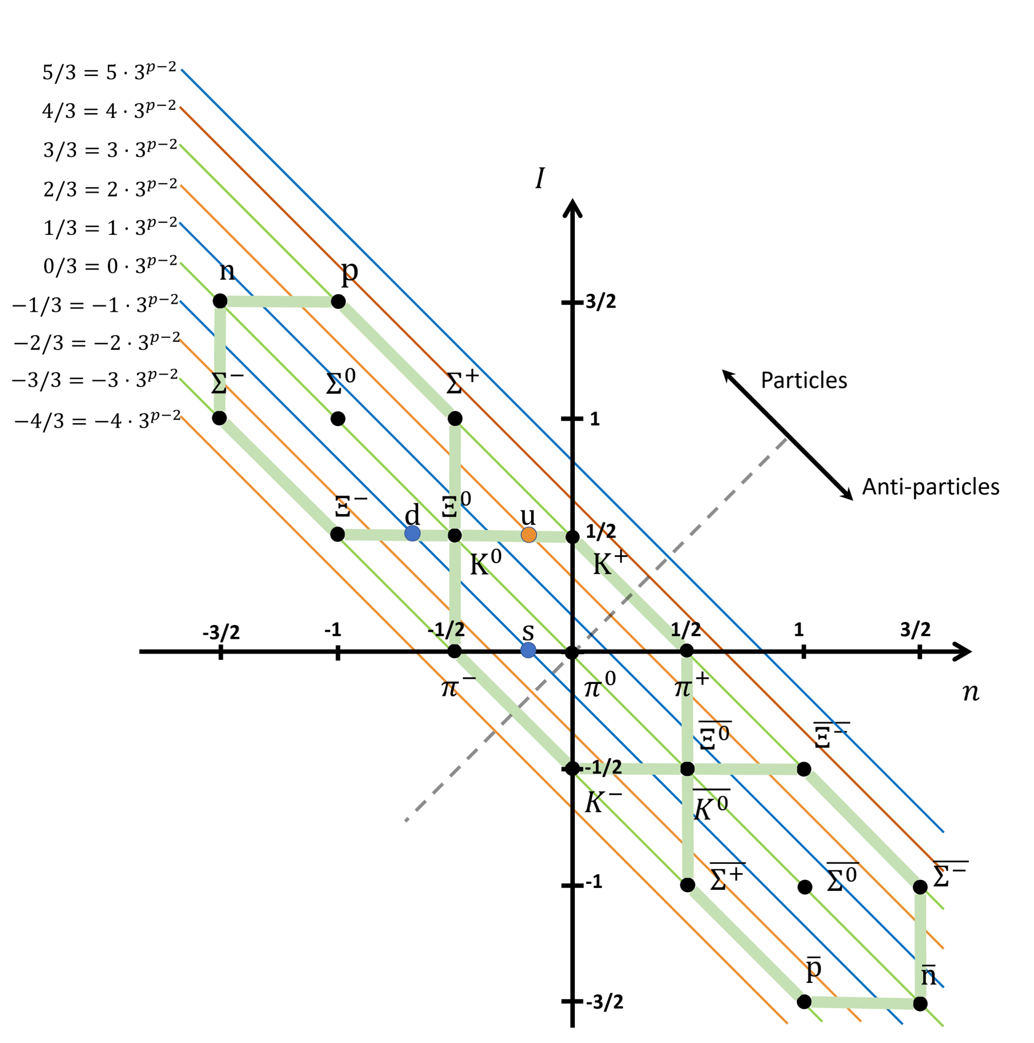
More generally, we can give a unified representation for arbitrary composit particles. First, we can give a representation of a single particle as . Likewise, a representation of particles with ( or higher) constituents is possible with
| (25) |
where are half-integers, or , is the identity map , and maps to the conjugate group with coefficients (c.f. References Brauer and Nesbitt 1941; Coish 1959). Then, the charge number is given by where plus and minus correspond to and , respectively. This includes a representation of mesons, baryons, pentaquark, and so on, in a unified way.
VI Quark Confinement
Finally, we provide a possible approach toward quark confinement which ascribes to fractionality in Galois field.
Suppose for the moment that up-quark and down-quark can be described by the following irreducible representation of :
| (26) |
We expect that proton and neutron can be expressed as and , respectively. Then, the quantum numbers of proton and neutron can be written in terms of their constituent quarks as follows:
| (27) | ||||
| (28) | ||||
| (29) |
Substitute this decomposition into Equation (23) and we obtain
| (30) |
Then, we can solve for and
| (31) |
Taking the values , and as in Table 2 we obtain
| (32) |
which are not half-integers as in (15). Therefore, irreducible representations of quarks as in Equation (26) is not possible.
Now, suppose that we can nevertheless write the corresponding charge numbers as elements of . Then, we obtain and . Counterintuitively, these fractional quantum numbers in are very large, which can be shown as follows. The modular inverses in of an integer in is defined by
| (33) |
On the other hand, from Fermat’s little theorem
| (34) |
we obtain
| (35) |
The prime given by Equation (2) contains the first odd prime , so it has the form for some . In this case, the fractional number in takes the value (see Figure 3). Therefore, fractional numbers in Galois field are large numbers of order . Consequently, isolated quark can have, for instance a huge electromagnetic self-energy (Figure 4). In this case, quark confinement in may be a consequence of energy minimization.


VII Discussion and Conclusions
Finally, we summarize and discuss our results. The NNG formula is a phenomenological equation. By using a Galois field, the NNG Formula (24) is rewritten as (23). The new quantum number , which includes isospin and hypercharge , arises from the multivaluedness of a linear representation of the Galois field. We also discussed quark confinement which ascribes to fractionality of Galois field. After all, these results may indicate finiteness and discreteness of the world. While such a method is unconventional, it is not inherently inconsistent under one assumption, namely that the geometry constructed by the real numbers is only an approximation of a finite and discrete geometry R.Penrose 2004; Ahmavaara 1965.
As future developments, we expect that composite particles such as pentaquarks Nakano et al. 2003; Aaij et al. 2016; Kim et al. 2017 can be explained by generalizing Equation (25) to any number of particles and combining the quantum numbers and to a single “grand spin” as discussed in Kim et al. 2017. We expect that the inclusion of other flavors such as c (charm), t (top) and b (bottom) would require extension of our result to (analogous to SU(3)), , and so on, which goes in parallel to the extension of SU(2) to SU(3) or higher. Representation of particles in Figure 2 can be modified accordingly. This extention can be done based on previous studies Mark 1938 and using a method equivalent to the “enlarging lemma” Kempe et al. 2001. Recently, with the development of quantum information, Galois fields have begun to be used to construct space-time models as error-correcting codes Lévay and Holweck 2019. Further application of Galois fields is expected in the foundation of quantum physics Chang et al. 2014 and time crystal with discrete space-time symmetry Shapere and Wilczek 2012; Wilczek 2012; Nakatsugawa et al. 2017; Nakatsugawa et al. 2020; Sacha and Zakrzewski 2018.
Acknowledgements.
We thank Kohkichi Konno, Masanori Yamanaka, Thomas Zeugmann, Tatsuhiko N. Ikeda, Masanori Morishita and Ryotaro Okazaki for stimulating and valuable discussions.References
- Yukawa (1966) H. Yukawa, Progress of Theoretical Physics Supplement 37-38, 512 (1966).
- Snyder (1947) H. S. Snyder, Phys. Rev. 71, 38 (1947).
- Finkelstein (1969) D. Finkelstein, Phys. Rev. 184, 1261 (1969).
- Luminet et al. (2003) J.-P. Luminet, J. R. Weeks, A. Riazuelo, R. Lehoucq, and J.-P. Uzan, Nature 425, 593 (2003).
- Coish (1959) H. R. Coish, Phys.Rev. 114, 383 (1959).
- Nambu (1987) Y. Nambu, in Quantum Field Theory and Quantum Statistics, Vol. 1, edited by I. A. Batalin (IOP Publishing, 1987) pp. 625–636, also in Broken Symmetry, World Scientific Pub Co Inc, 1995.
- Järnefelt (1977) G. Järnefelt, Astronomische Nachrichten 298, 69 (1977).
- Beltrametti and Blasi (1968) E. G. Beltrametti and A. A. Blasi, J. Math. Phys. 9, 1027 (1968).
- Shapiro (1960) I. S. Shapiro, Nuclear Phys 21, 474 (1960).
- Joos (1964) H. Joos, J. Math. Phys. 5, 155 (1964).
- Ahmavaara (1965) Y. Ahmavaara, J. Math. Phys. 6, 87 (1965).
- Morris (1974) H. C. Morris, Int. J. Theor. Phys. 9, 369 (1974).
- Lev (2010) F. M. Lev, Symmetry 2, 1810 (2010).
- Lev (2020) F. M. Lev, Symmetry 12, 409. (2020).
- Vladimirov et al. (1994) V. S. Vladimirov, I. V. Volovich, and E. I. Zelenov, p-Adic Analysis and Mathematical Physics (World Scientific, 1994) pp. 1–141.
- Kato et al. (2005) K. Kato, S. Kurokawa, and T. Saito, Number Theory I (Iwanami-Shoten, 2005) (in Japanese).
- R.Penrose (2004) R.Penrose, The road to reality (Vintage, 2004) Chap. 16.
- Amelino-Camelia (2010) G. Amelino-Camelia, Symmetry 2, 230 (2010).
- Järnefelt (1951) G. Järnefelt, Ann. Acad. Sci. Fennicae Ser. A.I. 96, 1 (1951).
- Shapere and Wilczek (2012) A. Shapere and F. Wilczek, Phys. Rev. Lett. 109, 160402 (2012).
- Wilczek (2012) F. Wilczek, Phys. Rev. Lett. 109, 160401 (2012).
- Nakatsugawa et al. (2017) K. Nakatsugawa, T. Fujii, and S. Tanda, Phys. Rev. B 96, 094308 (2017).
- Nakatsugawa et al. (2020) K. Nakatsugawa, T. Fujii, A. Saxena, and S. Tanda, J. Phys. A 53, 025301 (2020).
- Sacha and Zakrzewski (2018) K. Sacha and J. Zakrzewski, Rep. Prog. Phys. 81, 016401 (2018).
- Kustaanheimo (1952) P. Kustaanheimo, Ann. Acad. Sci. Fennicae Ser. A.I. 129, 1 (1952).
- Weinberg (2005) S. Weinberg, The Quantum Theory of Fields, Volume 1: Foundations (Cambridge University Press, 2005).
- Brauer and Nesbitt (1941) R. Brauer and C. Nesbitt, Ann. Math. 42, 556 (1941), sec. 30.
- Nakano et al. (2003) T. Nakano et al., Phys. Rev. Lett. 91, 012002 (2003).
- Aaij et al. (2016) R. Aaij et al., Phys. Rev. Lett 117, 202007 (2016).
- Kim et al. (2017) H.-C. Kim, M. V. Polyakov, and M. Praszałowicz, Phys. Rev. D 96, 014009 (2017).
- Mark (1938) J. C. Mark, On the modular representation of the group GLH, Ph.D. thesis, University of Toronto (1938).
- Kempe et al. (2001) J. Kempe, D. Bacon, D. A. Lidar, and K. B. Whaley, Phys. Rev. A 63, 042307 (2001).
- Lévay and Holweck (2019) P. Lévay and F. Holweck, Phys. Rev. D 99, 086015 (2019).
- Chang et al. (2014) L. N. Chang, Z. Lewis, D. Minic, and T. Takeuchi, Int. J. Mod. Phys. A 29, 1430006 (2014).