Quantum state preparation of spin eigenstates including the Dicke states with generalized all-coupled interaction in a spintronic quantum computing architecture
Preprint: APS/123-QED

The total spin angular momentum $\bm{S}$ is defined as the tensor sum, $\bm{S}=\sum_{i}\bm{S}_{i}$, where $\bm{S}_{i}$ denote spin operator of $i^{th}$ qubit. We will denote the spin eigenstates by $\ket{X(n,S,M)}$, where n is number of qubits, and S and M denote the spin and z-component of spin, quantum numbers i.e. $\bm{S}^{2}\ket{X(n,S,M)}=S(S+1)\hbar^{2}\ket{X(n,S,M)}$ and $\bm{S}_{z}\ket{X(n,S,M)}=M\hbar\ket{X(n,S,M)}$. We will denote the two single qubit states, $S=1/2,M=\pm 1/2$ by $\ket{0}$ and $\ket{1}$ respectively. The eigenstates of n-1 qubit system with spin S and a single qubit can be combined to yield eigenstates with spin of $S\pm(1/2)$. This is expressed in Eq. 1 (See Ref. (Pauncz 1979)) where we have defined $A=\sqrt{\frac{S+M+1}{2S+1}}$ and $B=\sqrt{\frac{S-M}{2S+1}}$. The state is normalized as $A^{2}+B^{2}=1$. It should be noted that the values of n,S and M may not specify a unique state, and this issue is dealt with later. The equations Eq. 1 a and b can be inverted as given in Eq. 2

We now assume that we have two kinds of Hamiltonians at our disposal and show that spin eigenfunction of n-qubit system can be prepared from n-1 qubit system by subjecting the later system to time evolutions under these two Hamiltonians. The two Hamiltonians we need are: 1) Heisenberg exchange interaction between all pairs of qubits 2) Zeeman interaction generated by local magnetic fields along z direction acting on the qubits. We have shown in Ref. (Sharma and Tulapurkar 2020) that both these Hamiltonians can be engineered in a system of non-interacting spin qubits connected to ferromagnetic reservoirs. This aspect is further discussed in section III. It should be noted that the first Hamiltonian can be used for entangling the qubits, while the second Hamiltonian can be used for single qubit z-axis rotation operation. The first Hamiltonian can be written as:

where $J^{\prime}$ denotes the exchange interaction strength. The above equation shows that eigenstates $\bm{S}^{2}$ operator are also eigenstates of all coupled Heisenberg Hamiltonian with eigenvalue $(J^{\prime}\hbar^{2}/2)[S(S+1)-3n/4]$. Let us now see how we can prepare state $\ket{X(n,S+1/2,M+1/2)}$ from $\ket{X(n-1,S,M)}$ state. We append a qubit in $\ket{0}$ state to the system and take the initial state as a tensor product state $\ket{\psi(0)}=\ket{X(n-1,S,M)}\otimes\ket{0}$. We now subject the initial state to time evolution under the all coupled Heisenberg interaction. As the states $\ket{X(n,S\pm 1/2,M+1/2}$ are eigenfunctions of the Hamiltonian, the state at time $t$ can be written as,

with $c_{1}(0)=A$ and $c_{2}(0)=-B$. From equation 1a and 1b, we see that both the spin-eigenstates are linear combinations of $\ket{X(n-1,S,M)}\otimes\ket{0}$ and $\ket{X(n-1,S,M+1)}\otimes\ket{1}$. We can therefore write the state at time $t$ as:

with appropriately normalized $a_{1}$ and $a_{2}$ factors. We can easily get the expressions for $a_{1}$ and $a_{2}$ in terms of $c_{1}$ and $c_{2}$ (and vice-versa) from equations 1 and 2, as given below:

Under the evolution with all coupled Heisenberg interaction, ignoring the global phase, we can write $c_{1}(t)=\exp(-i\omega t)c_{1}(0)$ and $c_{2}(t)=c_{2}(0)$, where $\omega=(E_{1}-E_{2})/\hbar$ and $E_{1}$ and $E_{2}$ are eigenvalues of $\ket{X(n,S+1/2,M+1/2)}$ and $\ket{X(n,S-1/2,M+1/2)}$ states respectively. $\omega$ is given by, $\omega=J^{\prime}(S+1/2)\hbar$. We can obtain $a_{1}(t)$ and $a_{2}(t)$ from equation 6 as $a_{1}(t)=A^{2}[\exp(-i\omega t)-1]+1$ and $a_{2}(t)=AB[\exp(-i\omega t)-1]$. We stop the time evolution at time $t_{s}$, when the amplitudes are given by $|a_{1}(t_{s})|=A$ and $|a_{2}(t_{s})|=B$. ( Normalization of the state imply that if $|a_{1}|=A$ then $|a_{2}|=B$ and vice-versa). Using the above expressions for $a_{1}$ or $a_{2}$, we get the following equation for $t_{s}$:

The state time time $t_{s}$ is very close to the desired $\ket{X(n,S+1/2,M+1/2)}$ state except for a relative phase factor. The state $\ket{\psi(t_{s})}$, ignoring the global phase, can be written as:

The relative phase factor $e^{i\phi}=(A/B)(a_{2}(t_{s})/a_{1}(t_{s}))$ can be easily corrected by applying local magnetic field to the last qubit for a certain time. This corresponds to application of $R_{z}(\theta)$ gate on the last qubit, which performs a rotation about z-axis, modifies the relative phase factor to $e^{i(\phi+\theta)}$ in Eq. 8. This clearly leads to the desired spin eigenstate for a rotation amount $\theta=2m\pi-\phi$ for any integer m. Eq. 7 besides providing the value of $t_{s}$ also gives the condition on S and M for which the algorithm would work. It can be easily checked that for real values $t_{s}$, the equation can be satisfied only when $2S+4M+3\geq 0$. In the above, we prepared $\ket{X(n,S+1/2,M+1/2)}$ state staring from$\ket{X(n-1,S,M)}$ state and appending a qubit in $\ket{0}$ state. The final state essentially corresponds to the first term in Eq. 2a. By appropriately choosing the stopping time $t_{s}$, followed by single qubit rotation of the last qubit, we can as well prepare $\ket{X(n,S-1/2,M+1/2)}$ state which corresponds to the second term in Eq. 2a. The stopping time in this case is chosen by to satisfy the condition $|a_{1}(t_{s})|=B$ or $|a_{2}(t_{s})|=A$. This condition gives the following equation for $t_{s}$:

The state at time $t_{s}$ is very close to the desired $\ket{X(n,S-1/2,M+1/2)}$ state except for a phase factor. The state $\ket{\psi(t_{s})}$ can be written as

As before, the relative phase factor can be corrected by single qubit rotation on the last qubit. The algorithm would work for real values of $t_{s}$, which gives the condition that $2(S-2M)\geq 1$.

Now if we examine Eq. 2b, we see that we can append a qubit in $\ket{1}$ state (instead of $\ket{0}$ state) to the n-1 qubit spin-eigenstate and prepare n qubit spin-eigenstates. The algorithm is again same as before: The system is subjected to the evolution under all coupled Heisenberg Hamiltonian for a certain time followed by phase correction by single qubit rotation operation on the last qubit. We will write the same equations as 4 and 5 with difference that $c_{1}(0)=B$ and $c_{2}(0)=A$. Putting $c_{1}(t)=c_{1}(0)\exp(-i\omega t)$ and $c_{2}(t)=c_{2}(0)$ in equation 6, we get $a_{1}(t)=AB[\exp(-i\omega t)-1]$ and $a_{2}(t)=B^{2}[\exp(-i\omega t)-1]+1$. We stop the time evolution at time $t_{s}$, when the amplitudes are given by $|a_{1}(t_{s})|=A$ and $|a_{2}(t_{s})|=B$ if desired final state is $\ket{X(n,S+1/2,M+1/2)}$. We get:

If the final desired state is $\ket{X(n,S-1/2,M+1/2)}$, the time evolution is stopped when $|a_{1}(t_{s})|=B$ and $|a_{2}(t_{s})|=A$. We get:

Let us now examine the case where spin quantum number is increased by 1/2 i.e. preparation of $S+1/2$ spin state from $S$ spin-state. We shall call it the spin incrementing method from now on. This can be done in two ways as discussed above: We can prepare $\ket{X(n,S+1/2,M+1/2)}$ state from $\ket{X(n-1,S,M)}$ or $\ket{X(n-1,S,M+1)}$ by appending $\ket{0}$ or $\ket{1}$ respectively. Calling the final state quantum numbers as $\widetilde{S}=S+1/2$ and $\widetilde{M}=M+1/2$, and using equations 7 and 11, we see that the two schemes work under the respective conditions: $\widetilde{S}+2\widetilde{M}\geq 0$ and $\widetilde{S}-2\widetilde{M}\geq 0$. It is thus always possible to reach the final state using one of these two or both expansion schemes. We can similarly examine the case where the final state spin quantum number is decreased by 1/2. In the same spirit, we can call this the spin decrementing method. This again can be done in two ways: We can prepare $\ket{X(n,S-1/2,M+1/2)}$ state from $\ket{X(n-1,S,M)}$ or $\ket{X(n-1,S,M+1)}$ by appending $\ket{0}$ or $\ket{1}$ respectively. Calling the final state quantum numbers as $\widetilde{S}=S-1/2$ and $\widetilde{M}=M+1/2$, and using equations 9 and 12, we see that the two algorithms work under the respective conditions $\widetilde{S}-2\widetilde{M}+1\geq 0$ and $\widetilde{S}+2\widetilde{M}+1\geq 0$. It is thus always possible to reach the final state using one of these two or both algorithms.

We now address the problem mentioned earlier that n,S and M quantum numbers may not be sufficient to specify a state completely. We can use a ”branching diagram” to represent a spin-eigenstate. (See Ref. Pauncz 1979 for details). We essentially construct a state starting from one qubit state and increasing the number of electrons in each stage, using either equation 1 a or 1 b. Thus in each stage we either increase or decrease spin by 1/2. Specifying the path of how a state is constructed, specifies the state uniquely. Increasing spin step is denoted by 1 and decreasing spin step is denoted by 2. As an example, let’s consider state $\ket{X(n=5,S=3/2,M=1/2,11211)}$. The state $\ket{X(n=5,S=3/2,M=1/2)}$ has a degeneracy of 5 and path 11211 is required to specify the state uniquely (This state turns out be $\sqrt{(1/18)}[2\ket{00101}+2\ket{00110}-\ket{01001}-\ket{01010}+\ket{01100}-\ket{10001}-\ket{10010}+\ket{10100}-2\ket{11000}]$). To prepare this state on a quantum computer (equipped with the two Hamiltonians mentioned before), we essentially follow the same path viz. 11211. In each step there could be two possible ways to prepare the next state. Let’s trace back the path starting with the final state. We need to follow path of increasing spin i.e. we can prepare the final state from $\ket{X(n=4,S=1,M=0,1121)}$ or $\ket{X(n=4,S=1,M=1,1121)}$ by appending $\ket{0}$ or $\ket{1}$ respectively. Both of these options are allowed as they satisfy $\widetilde{S}+2\widetilde{M}\geq 0$ and $\widetilde{S}-2\widetilde{M}\geq 0$ conditions. Let’s choose to prepare the final state from $\ket{\psi_{4}}=\ket{X(n=4,S=1,M=0,1121)}$. To prepare $\ket{\psi_{4}}$ we need to follow the path of increasing spin, which means that it can be prepared from $\ket{X(n=3,S=1/2,M=-1/2,112)}$ or $\ket{X(n=3,S=1/2,M=1/2,112)}$ by appending $\ket{0}$ or $\ket{1}$ respectively. Both the options are allowed. Let’s choose to prepare the $\ket{\psi_{4}}$ state from $\ket{\psi_{3}}=\ket{X(n=3,S=1/2,M=1/2,112)}$. To prepare $\ket{\psi_{3}}$, we need to follow spin decreasing path i.e. the state can be prepared from $\ket{X(n=2,S=1,M=0,11)}$ or $\ket{X(n=2,S=1,M=1,11)}$ by appending $\ket{0}$ or $\ket{1}$ respectively. Again both these options are allowed. If we choose $\ket{\psi_{2}}=\ket{X(n=2,S=1,M=1,11)}$, then we have finished the process as $\ket{\psi_{2}}=\ket{00}$ is a completely un-entangled state. If we choose $\ket{\psi_{2}}=\ket{X(n=2,S=1,M=0,11)}$, we need one more step to prepare $\ket{\psi_{2}}$ from $\ket{1}$ or $\ket{0}$ by following spin increasing path. It is clear from above arguments that we can prepare a general spin-eigenstate of n-qubit system in O(n) stages with each stage involving an entangling evolution under all coupled Heisenberg interaction followed by single qubit rotation operation. We shall see later how this linear step algorithm can be improved for a special class of spin-eigenstates called Dicke states.

Let’s consider preparation of state $\ket{X(n,S=n/2,M)}$. This is the state with highest value of spin and the path to be followed to prepare it, is always spin-increasing i.e. we do not need to specify the path separately. As a particular example, let’s choose $M=S-2=(n-4)/2$. This state can be prepared from $\ket{X(n-1,S=(n-1)/2,M=(n-5)/2}$ or $\ket{X(n-1,S=(n-1)/2,M=(n-3)/2}$ by appending $\ket{0}$ or $\ket{1}$ respectively. However, state $\ket{X(n-1,S=(n-1)/2,M=(n-3)/2}$ can not be used as it does not satisfy the condition $\widetilde{S}-2\widetilde{M}\geq 0$. For the same reason, even the state $\ket{X(n-1,S=(n-1)/2,M=(n-3)/2}$ can not be prepared from $\ket{X(n-1,S=(n-2)/2,M=(n-2)/2}$ by appending $\ket{1}$. However if it was possible to prepare these states by these ’forbidden’ paths, it would be of a great advantage as the state $\ket{X(n-1,S=(n-2)/2,M=(n-2)/2}$ is completely un-entangled. This means that we could have prepared $\ket{X(n,S=n/2,M=(n-4)/2)}$ state in just two steps. The same considerations apply to preparation of $\ket{X(n,S=n/2,M=(-n+4)/2)}$ starting from $\ket{X(n,S=n/2-2,M=-n/2)}$ appending $\ket{0}$ states, which is a completely un-entangled state (product state).

To find a solution to this problem, let us take the case of preparing $\ket{X(n,S+1/2,M+1/2)}$ state from $\ket{\psi_{i}}=\ket{X(n-1,S,M+1)}\otimes\ket{1}$ and understand the constraint $2(S-2M)\geq 1$ from a different perspective. By using the equation 2b, we can find out the average value spin angular momentum of the initial state as $\braket{\psi_{i}|\bm{S}^{2}|\psi_{i}}=\hbar^{2}[S(S+1)-M-1/4]$. The intermediate state ($\ket{\overline{\psi}}$ after the entangling evolution is given by equation 8. If we can reach the intermediate state $\ket{\overline{\psi}}$, we can certainly reach the final desired state by correcting for the phase $\phi$ by single qubit operation. The average spin angular momentum of the intermediate state can be found out using Eq. 2. After some algebraic steps, one can show that

As the spin angular momentum is conserved during the evolution under all coupled Heisenberg interaction, the second therm on RHS of the above equation must be zero, which gives us a condition:

Comparing this to equation 12, we see that the phase correction required is the same as $\omega t_{s}$. Further, the requirement that $\phi$ be real gives us the same condition as obtained before viz. $2(S-2M)\geq 1$. It should be noted that the spin angular momentum of the desired final state, $\ket{X(n,S+1/2,M+1/2)}$ given by $(S+1/2)(S+3/2)\hbar^{2}$, is always greater than that of the initial state. The difference, $(S+M+1)\hbar^{2}$ is actually supplied to the system during the phase correction step through single qubit operations which tends to make $\phi=0$. Thus the algorithms that we have used essentially work as follows: The initial state is subjected to entangling evolution. Spin momentum is conserved in this process. Then the state is subjected to z-axis rotation of last qubit. This step changes the spin momentum of the state. If the spin momentum after these two steps can reach the desired final state spin momentum, the expansion is successful. If the spin momentum of the final state can not reach the spin momentum of the desired final state, what we can do is to repeat the previous two steps i.e. subject the state to entangling evolution for a certain time and then z-axis rotation of the last qubit. We repeat these steps till the spin momentum of the evolved state reaches the final state spin momentum. Note that there is a limitation to how much spin momentum can be pumped using single qubit rotations (dependent on the current state) and hence we need to go through these processes iteratively to pump in more and more spin momentum. This redressal can be summarized as a schematic illustrated in Fig. 1 where we have simply appended a loop in the previous sequence of operations.

A rigorous way to appreciate the workings of this modification is to track the states throughout. Like seen before, tracking the coefficients $c_{1}(t),c_{2}(t),a_{1}(t)$ and $a_{2}(t)$ is sufficient for this purpose. It is also worth emphasising here that $(c_{1}(t),c_{2}(t))$ can be considered as a (complex) coordinate vector of the state at time t in the basis {$\ket{X(n,S+1/2,M+1/2}$, $\ket{X(n,S-1/2,M+1/2}$}. Studying time evolutions under all coupled Heisenberg interaction is easy in this basis. A state evolved for a time $t_{s}$ can be simply represented by the coordinate $\left(c_{1}(t)\exp(-i\omega t_{s}),c_{2}(t)\right)$ ignoring a global phase. Similarly, the coordinate $(a_{1}(t),a_{2}(t))$ in {$\ket{X(n-1,S,M}\otimes\ket{0}$, $\ket{X(n-1,S,M+1}\otimes\ket{1}$} basis is easy to work with, when studying the effect of single qubit rotation $R_{z}$ of the added qubit. A rotation by an amount $\theta$ transforms the coordinate to $\left(a_{1}(t)\exp(-i\theta),a_{2}(t)\right)$ where we have neglected the global phase again. Also, since we already have a way to transform the coordinate vectors into the other basis after either evolution or rotation operation (Eq. 6), we can find the state coordinates at any time during the iteration starting from the initial state $\ket{\psi_{i}}$ which is represented as $(c_{1}(0),c_{2}(0))=(B,A)$ and $(a_{1}(0),a_{2}(0))=(0,1)$ in respective bases.

The choice of $t_{s}$ and $\phi$ in each iteration that minimizes the total number iterations required to prepare the desired state is an important question. We observe that except for the last iteration, choosing $t_{s}=\pi/\omega$ and $\theta=\pi$ takes the coefficients closest to the desired state coordinates $(c_{1},c_{2})=(1,0)$ and $(a_{1},a_{2})=(A,B)$ in respective bases for given values of S and M and hence A and B (See Appendix. A). For this choice, the coefficients in the two bases at the end of $(r+1)$th iteration in terms of those at the end of $r$th iteration can be obtained as:

where we have discretely indexed the coefficients using square brackets indicating a sampling of their continuous counterparts at the end of each iteration. For r = 0 the sampling is done at t=0 i.e. $c_{1}[0]$ is defined as $c_{1}(0)$ and so on. Eq. 15 is suggestive of a rotation of the coordinate vector by same amount, say $\alpha$, in either basis and can be easily by choosing to write $(A,B)=(\cos(\alpha/2),\sin(\alpha/2))$. Further insight can be gained by visualizing these operations and hence the rotations geometrically and is discussed in detail in Appendix. A. The key understanding is that the sequence of operations $(I\otimes R_{z}(\pi))U(\pi/\omega)$, can be compared to a Grover’s iterate, with the time evolution $U(\pi/\omega)$ seen as an instance of an oracle and the single qubit rotation $R_{z}(\pi)$ as an instance of the reflection operation about the initial state vector instead of the usual reflection about the mean operation (also known by the name diffusion operation). The initial iterations progresses identically to Grover’s algorithm amplifying $c_{1}$, the component along $\ket{X(n,S+1/2,M+1/2)}$, in each iteration and hence pumping in the spin momentum described previously. This prepares the state to within an error probability of $\frac{S-M}{2S+1}$ in $O\left(\sqrt{\frac{2S+1}{S-M}}\right)$ iterations. However, this error can be corrected completely in the last iteration. In the last iteration the evolution interval and the amount of rotation is chosen in a way discussed in previous section: Solving $|a_{1}(t_{s})|=A$ (or $|a_{2}(t_{s})|=B$) for $t_{s}$ after the entangling evolution and determining the relative phase between $a_{1}$ and $a_{2}$ immediately after the entangling evolution. The final iteration thus gives us the desired state: $\ket{X(n,S+1/2,M+1/2)}$.

The above amplitude amplification scheme generalizes the spin incrementing expansion of a $\ket{1}$ appended spin-eigenstate $\ket{n-1,S,M+1}$ outside the region $2(S-2M)\geq 1$ and reduces to the single iteration expansion inside the region as discussed in previous section. Although we have discussed here one of the four spin-incrementing and decrementing methods, it is also possible to generalize other expansion methods using the same procedure in respective ’forbidden’ regions.

Here, we summarize the expansion methods discussed above in the context of highly-entangled largest-spin-valued eigenstates (called Dicke states) and evaluate its cost of preparation from completely unentangled states.

For a system of n qubits, in the notation we have used here, Dicke states can be written as $\ket{X(n,S=n/2,M=n/2-k)}$. The index $0\leq k\leq n$ is called the hamming weight and for $k=0$ and $n$ correspond to unentangled spin-eigenstates that are trivial to prepare. We will also use a relatively common shorthand $D^{n}_{k}$ to denote these states from now on. We must use spin-incrementing path in preparing these states and the methods discussed in Section. II.1, can be translated as

1. 1.

   Weight preserving:
   $D^{n}_{k}\xrightarrow{\otimes\ket{0}}D^{n}_{k}\otimes\ket{0}\xrightarrow{U}\bar{D}^{n+1}_{k}\xrightarrow{\text{Phase Correction}}D^{n+1}_{k}$

2. 2.

   Weight incrementing:
   $D^{n}_{k}\xrightarrow{\otimes\ket{1}}D^{n}_{k}\otimes\ket{1}\xrightarrow{U}\bar{D}^{n+1}_{k+1}\xrightarrow{\text{Phase Correction}}D^{n+1}_{k+1}$

For convenience we have chosen to write the expansion methods starting from an n qubit state instead of n-1 qubit state. We have also dubbed the expansion of a $\ket{0}$ and $\ket{1}$ appended eigenstate as weight preserving and incrementing expansion respectively. The respective requirements on $\widetilde{S}$ and $\widetilde{M}$ can also be translated in terms of n and k as $k\leq 3(n+1)/4$ and $k\geq(n-3)/4$ in respective cases. These expansions can be visualized in an n-k space where each coordinate $(n,k\leq n)$ represents a Dicke state $D^{n}_{k}$. Here, tracing points horizontally (diagonally) towards right (positive slope direction) corresponds to weight preserving (incrementing) expansion. Corresponding regions where aforementioned movement is feasible are shaded green and pink respectively in Fig. 2. The dark coloured region indicates the simultaneous feasibility of two expansions and therefore it is possible to expand in either direction for points in this region. The blue coloured line borders the entangled states inside. Thus, the task of preparing an arbitrary Dicke state essentially translates to finding out a path from $(n,k)$ to any point outside the blue border representing all zeros or all ones states. It can be seen that the weight preserving and incrementing expansions are not sufficient individually to prepare arbitrary Dicke states but are sufficient when used together. As an example, consider preparation of $D^{34}_{10}$ state. As shown in Fig. 2, we back trace diagonally till point (31,7) and then horizontally until we reach (9,7). And finally we back trace diagonally to point (2,0). This is also evident from preparation of $D^{33}_{7}$ and $D^{35}_{28}$, whose preparation paths are also shown in Fig. 2. Based on this observations, we can write a particularly simple linear-step algorithm to prepare arbitrary Dicke states in terms of finding a path to unentangled states: Back trace diagonally as far as possible, then back trace horizontally as far as possible and repeat these steps.

In Section. II.2 we discussed amplitude amplification can be used to expand eigenstates in the ’forbidden’ regions. In the present context this means we can continue to trace a path diagonally backwards inside green region as well expecting to reach an unentangled state quicker. For the example of preparing $D^{34}_{10}$ considered above, we traced back a path to (31,7) but using amplitude amplification we can trace a path all the way back to (25,1) and hence (24,0) which is an simple product state $\ket{0}^{\otimes 24}$ (See Fig. 2). Although, we reach an unentangled state in $k=10$ spin-incrementing steps here, we should note that each weight incrementing expansion (using amplitude amplification) in the green region becomes costlier, requiring more number of iterations (r), for decreasing k and therefore a sum of iterations in each step of the traced path is a better indicator of the cost. Also, since the cost of preparing $D^{n}_{1}$, which is a W state, from $D^{n-1}_{0}$ is $O(\sqrt{n})$, we may as well choose to prepare these W states exponentially faster using algorithms like discussed in Ref. (Sharma and Tulapurkar 2020) in $O(\log(n))$ steps. The cost for preparing $D^{n}_{1}$ from $D^{n-1}_{0}$ is obtained by noting that preparing $D^{n+1}_{k+1}$ from $D^{n}_{k}$ requires $O\left(\sqrt{\frac{2\widetilde{S}}{\widetilde{S}-\widetilde{M}}}\right)\approx O\left(\sqrt{\frac{n+1}{k+1}}\right)$ iterations, where we have substituted $\widetilde{S}=(n+1)/2$ and $\widetilde{M}=(n+1)/2-(k+1)$.

We can now describe our final algorithm to prepare arbitrary Dicke states. For $k<n/2$, first prepare $D^{n-k+1}_{1}$ state in $\lceil\log_{4}(n-k+1)\rceil$ number of stages as described in Sharma and Tulapurkar 2020, then use the generalized weight incrementing method to successively prepare Dicke states with increasing ”spin-down” number (climbing diagonally upwards in Fig. 2). The number of stages required for each climb is the number of convergence steps and is added up cumulatively with each climb upto the point (n,k). Note that r automatically becomes 1 when in pink region. The total time cost (number of stages) to prepare (n,k) can thus be given by:

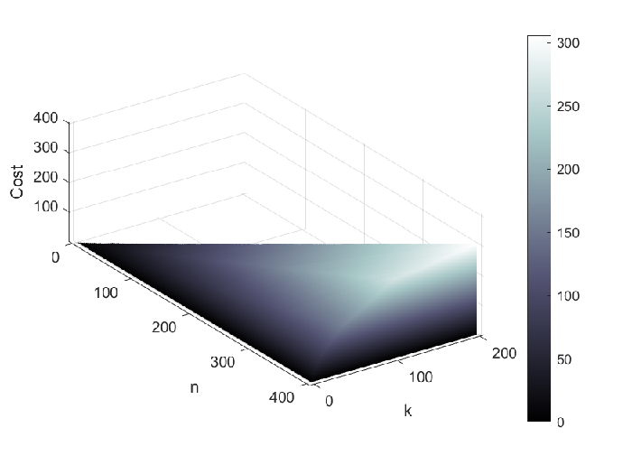
where $r_{(p,q)}$ indicates number of iterations required to prepare $D^{p}_{q}$ from $D^{p-1}_{q-1}$. The exact cost in order to prepare $D^{n}_{k\leq n/2}$ using this scheme is plotted in Fig. 3 for some values n and k. We see that the cost is always less than n and this algorithm performs significantly better than the linear step algorithm discussed previously for smaller and smaller values of k. The sub-linearity of this cost for some values of k is discussed in Appendix. C. On the other hand, for $k>n/2$, prepare $D^{n}_{n-k}$ using the method above and then apply bit-flip gates to all the qubits. An analogous approach to prepare $D^{n}_{k>n/2}$ would to be to first prepare one-spin-up W states exponentially (also suggested in Ref. (Sharma and Tulapurkar 2020)) and then repeatedly use weight preserving expansion and if needed using amplitude amplification.

As an example of using this final algorithm, a path to prepare $D^{34}_{10}$ state is shown in Fig. 2. Starting from point (1,1) we first jump by maximum factor of 4 to reach point (25,1) i.e. $(1,1)\rightarrow(4,1)\rightarrow(16,1)\rightarrow(25,1)$. We then move diagonally till point (31,7) by using spin angular momentum pumping algorithm. From point (31,7) we move diagonally to point (34,10) by using weight incrementing method.

We now discuss generalization of Hamiltonian describing systems where the algorithm discussed can still be implemented. The algorithms we have discussed used two kinds of Hamiltonians viz. Heisenberg exchange interaction between all pairs of qubits and Zeeman interaction generated by local magnetic fields along z direction acting on the qubits. Zeeman Hamiltonian is diagonal in the computational basis. All coupled Heisenberg Hamiltonian (Eq. 3) commute with $\bm{S_{z}}$ and is block diagonal in the partitions of the computational basis with fixed value of k ($k=n/2-M$). We will call this as k-spin-down subspace which has dimension of ${}^{n}C_{k}$. In this subspace, the Hamiltonian is given by:

where $\ket{u}$ denotes a computational basis state comprising of string of 0’s and 1’s. ’$\cdot$’ represents the bitwise ’AND’. Actually, every diagonal entry of $\mathcal{H}_{k}$ can be shown to be $J(^{k}C_{2}+^{n-k}C_{2}-k(n-k))$ but note we have taken them to be 0, since they only contribute global phase factors in state evolutions. (We have defined $J$ as $J^{\prime}(\hbar/2)^{2}$ for simplicity.) The above Hamiltonian has dimension of ${}^{n}C_{k}$ with $k+1$ distinct eigenvalues corresponding to S varying from $n/2$ to $n/2-k$. Equation 17 essentially means that the Hamiltonian has non-zero values at only the indices corresponding to the basis states obtainable by single swaps of 1 and 0. A more general Hamiltonian in the k-spin-down subspace can be given as ($k\leq n/2$)

If we impose $J_{m}=0\;\forall\;m\neq l\in[0,k]$ above and denote the Hamiltonian (partial Hamiltonians) so obtained by $\mathcal{H}_{k,l}$, we can write $\mathcal{H}_{k}=\sum_{l=0}^{k}\mathcal{H}_{k,l}$. The partial hamiltonian $\mathcal{H}_{k,l}$ can be interpreted to represent the interaction between the states obtainable by l swaps of 1’s and 0’s in the binary literals representing these state. It can be seen that only $\mathcal{H}_{k,1}$ has been dealt with until now. The other partial Hamiltonians also have a similar symmetry as possessed by $\mathcal{H}_{k,1}$. Therefore, the expansion procedures, scope of their operations and the amplitude amplification algorithm work for each $\mathcal{H}_{k,l}$ independently ($l\neq 0,\mathcal{H}_{k,0}=I$). The only difference is that the value of $\omega=(E_{1}-E_{2})/\hbar$ depends on the $\mathcal{H}_{k,l}$ (See the discussion in Appendix. B). Further, the partial Hamiltonians commute with each other i.e. $[\mathcal{H}_{k,m},\mathcal{H}_{k,n}]=0$. Thus a Hamiltonian given by sum the partial Hamiltonians can also be used for all the algorithms discussed previously.