A Stochastic Control Approach to Defined Contribution Plan Decumulation:
“The Nastiest, Hardest Problem in Finance”
Abstract
We pose the decumulation strategy for a Defined Contribution (DC) pension plan as a problem in optimal stochastic control. The controls are the withdrawal amounts and the asset allocation strategy. We impose maximum and minimum constraints on the withdrawal amounts, and impose no-shorting no-leverage constraints on the asset allocation strategy. Our objective function measures reward as the expected total withdrawals over the decumulation horizon, and risk is measured by Expected Shortfall (ES) at the end of the decumulation period. We solve the stochastic control problem numerically, based on a parametric model of market stochastic processes. We find that, compared to a fixed constant withdrawal strategy, with minimum withdrawal set to the constant withdrawal amount, the optimal strategy has a significantly higher expected average withdrawal, at the cost of a very small increase in ES risk. Tests on bootstrapped resampled historical market data indicate that this strategy is robust to parametric model misspecification.
Keywords: optimal control, DC plan decumulation, variable withdrawal, Expected Shortfall, asset allocation, resampled backtests
JEL codes: G11, G22
AMS codes: 91G, 65N06, 65N12, 35Q93
1 Introduction
The traditional Defined Benefit (DB) pension plan is in the process of disappearing for new entrants into the labour market.11 1 See, for example, “The extinction of defined-benefit plans is almost upon us,” Globe and Mail, October 4, 2018. https://www.theglobeandmail.com/investing/personal-finance/retirement/article-the-extinction-of-defined-benefit-pension-plans-is-almost-upon-us/ In some countries, notably Australia, DB plans have been replaced by Defined Contribution (DC) plans almost exclusively. 22 2 In Australia, DC plans have 86% of pension assets, compared with 14% in DB assets.(Towers-Watson 2020)
Assuming the DC plan holder has accumulated a reasonable amount in her DC plan account, the retiree is faced with an enormous challenge. The retiree has to devise an investment policy and a withdrawal strategy during the decumulation phase. Nobel laureate William Sharpe has referred to DC plan decumulation as “the nastiest, hardest problem in finance” (Ritholz 2017).
Although it is often suggested that DC plan holders should purchase annuities upon retirement, this is rarely done (Peijnenburg et al. 2016). In fact, MacDonald et al. 2013 argue that in many instances, this entirely rational. Reasons for the lack of interest in annuities include meager returns of annuities in the current low interest rate environment, poor annuity pricing, the lack of true inflation protection, and no access to capital in the event of emergencies.
For an extensive review of strategies for decumulation, we refer the reader to Bernhardt and Donnelly 2018 and MacDonald et al. 2013. A non-exhaustive list of the approaches discussed by these authors include use of traditional utility functions, practitioner rules of thumb, target approaches, minimizing probability of ruin and modern tontines. Previous decumulation strategies are also summarized in Forsyth 2020b. Concerning the current state of DC plan decumulation strategies, MacDonald et al. 2013 conclude “There is no solution that is appropriate for everyone and neither is there a single solution for any individual.”
We should mention that there is a standard rule of thumb for DC plan decumulation, termed the four per cent rule. Based on historical backtests, Bengen 1994 suggests investing in a portfolio of 50% bonds and 50% stocks, and withdrawing 4% of the initial capital each year (adjusted for inflation). Over historical rolling year 30 year periods, this strategy would have never depleted the portfolio.
Another recent strategy is based on the Annually Recalculated Virtual Annuity (ARVA) (Waring and Siegel 2015; Westmacott and Daley 2015; Forsyth et al. 2020). The ARVA strategy determines the yearly spending based on the theoretical value of a fixed term (virtual) annuity purchased with the current portfolio wealth. This approach is efficient in the sense that the portfolio is exhausted at the end of the investment horizon, but there is no guarantee of a yearly minimum withdrawal amount.
A recent survey33 3 2017 Allianz Generations Ahead Study - Quick Facts #1. (2017), Allianz. showed that a majority of pre-retirees fear exhausting their savings in retirement more than death. In addition, it is considered axiomatic amongst practitioners that retirees desire to have minimum (real) cash flows each year to fund expenses (Tretiakova and Yamada 2011). Typical (e.g. CRRA) utility function based objective functions do not directly focus on these two issues.
To address these two concerns, our objective in this article is to determine a decumulation strategy which has the following characteristics.
- •
Withdrawals can be variable, but with minimum and maximum constraints.
- •
The risk of portfolio depletion is minimized.
- •
The expected average withdrawal is maximized.
- •
The asset allocation strategy can be dynamic and non-deterministic.
We specify that the withdrawals are to take place over a fixed, lengthy (30 years) decumulation horizon. We do not explicitly take into account longevity risk, which we recognize as a weakness of this strategy. However, this is mitigated (somewhat) by specifying a long decumulation period. For example, the probability that a 65-year old Canadian male attains the age of 95, is about . 44 4 www.cia-ica.ca/docs/default-source/2014/214013e.pdf
We pose the decumulation problem as an exercise in optimal stochastic control. We have two controls: the asset allocation and the withdrawal amount. These controls are time and state dependent. Our objective function is composed of a measure of reward and risk. Our measure of reward is the expected total withdrawals (EW) over the thirty year period. Our measure of risk is expected shortfall (ES) at the end of the decumulation period. The ES at level x% is the mean of the worst x% of outcomes. The negative of ES is also known as Conditional Value at Risk (CVAR) or Conditional Tail Expectation (CTE).
We emphasize that, in contrast to previous studies on DC plan decumulation (Forsyth et al. 2019; Forsyth et al. 2020), where deterministic withdrawal strategies are coupled with optimal asset allocation, in this work, we determine both the optimal withdrawal strategy and the optimal asset allocation.
We should note that a strategy using ES as a risk measure is formally a pre-commitment policy. Some authors have taken the point of view that pre-commitment polices are not time consistent, hence non-implementable. However, as noted in Forsyth 2020a, the time zero strategy based on a pre-commitment ES policy is identical to the strategy for an induced time consistent policy, hence is implementable.55 5 An implementable strategy has the property that the investor has no incentive to deviate from the strategy computed at time zero at later times (Forsyth 2020a). The induced time consistent strategy in this case is a target based shortfall. The concept of induced time consistent strategies is discussed in Strub et al. 2019. In fact, Forsyth 2020a shows that enforcing a time consistent constraint on policies which use ES as a risk measure has undesirable consequences. The relationship between pre-commitment and implementable target based schemes in the mean-variance context is discussed in Vigna 2014 and Menoncin and Vigna 2017.
We assume that the retiree has an investment portfolio consisting of a stock index and a bond index, and desires to maximize real (inflation adjusted) total withdrawals. We calibrate stochastic models of real stock and bond indexes to historical data over the 1926:1-2019:12 period. We assume yearly withdrawals and rebalancing of the DC account. We term the market where the assets follow the parametric model fit to the historical data the synthetic market.
We devise a numerical method for determining the optimal policies. We enforce realistic investment constraints (no shorting, no leverage) and maximum and minimum constraints on the yearly withdrawal amounts. Compared to a strategy with a fixed withdrawal amount per year, we find that a variable withdrawal strategy, with a minimum withdrawal set to the fixed withdrawal amount, has a significantly increased expected average withdrawal, with only a very small increase in ES risk.
We also test the robustness of the strategy computed in the synthetic market by carrying out tests using bootstrap resampled historical data (the historical market). The efficient EW-ES frontiers for both synthetic and historical market tests are very close, indicating that the strategy computed in the synthetic market is robust to model misspecification.
2 Formulation
We assume that the investor has access to two funds: a broad market stock index fund and a constant maturity bond index fund.
The investment horizon is . Let and respectively denote the real (inflation adjusted) amounts invested in the stock index and the bond index respectively. In general, these amounts will depend on the investor’s strategy over time, as well as changes in the real unit prices of the assets. In the absence of an investor determined control (i.e. cash withdrawals or rebalancing), all changes in and result from changes in asset prices. We model the stock index as following a jump diffusion.
In addition, we follow the usual practitioner approach and directly model the returns of the constant maturity bond index as a stochastic process, see for example Lin et al. 2015; MacMinn et al. 2014. As in MacMinn et al. 2014, we assume that the constant maturity bond index follows a jump diffusion process as well.
Let , i.e. is the instant of time before , and let be a random number representing a jump multiplier. When a jump occurs, . Allowing for jumps permits modelling of non-normal asset returns. We assume that follows a double exponential distribution (Kou 2002; Kou and Wang 2004). If a jump occurs, is the probability of an upward jump, while is the chance of a downward jump. The density function for is
| (2.1) |
We also define
| (2.2) |
In the absence of control, evolves according to
| (2.3) |
where is the (uncompensated) drift rate, is the volatility, is the increment of a Wiener process, is a Poisson process with positive intensity parameter , and are i.i.d. positive random variables having distribution (2.1). Moreover, , , and are assumed to all be mutually independent.
Similarly, let the amount in the bond index be . In the absence of control, evolves as
| (2.4) |
where the terms in equation (2.4) are defined analogously to equation (2.3). In particular, is a Poisson process with positive intensity parameter , and has distribution
| (2.5) |
and . , , and are assumed to all be mutually independent. The term in equation (2.4) represents the extra cost of borrowing (the spread).
The diffusion processes are correlated, i.e. . The stock and bond jump processes are assumed mutually independent. See Forsyth 2020b for justification of the assumption of stock-bond jump independence.
Remark 2.1 (Stock and Bond Processes).
An obvious generalization of processes (2.3) and (2.4) would be to include stochastic volatility effects. However, previous studies have shown that stochastic volatility appears to have little consequences for long term investors (Ma and Forsyth 2016). As a robustness check, we will (i) determine the optimal controls using the parametric model based on equations (2.3) and (2.4) and (ii) use these controls on bootstrapped resampled historical data, which makes no assumptions about the underlying bond and stock stochastic processes.
We define the investor’s total wealth at time as
| (2.6) |
We impose the constraints that (assuming solvency) shorting stock and using leverage (i.e. borrowing) are not permitted, which would be typical of a DC plan retirement savings account. In the event of insolvency (due to withdrawals), the portfolio is liquidated, trading ceases and debt accumulates at the borrowing rate.
3 Notational conventions
Consider a set of discrete withdrawal/rebalancing times
| (3.1) |
where we assume that is constant for simplicity. To avoid subscript clutter, in the following, we will occasionally use the notation and . Let the inception time of the investment be . We let be the set of withdrawal/rebalancing times, as defined in equation (3.1). At each rebalancing time , , the investor (i) withdraws an amount of cash from the portfolio, and then (ii) rebalances the portfolio. At , the final cash flow occurs, and the portfolio is liquidated. In the following, given a time dependent function , then we will use the shorthand notation
| ; | (3.2) |
We assume that there are no taxes or other transaction costs, so that the condition
| ; | (3.3) |
holds. Typically, DC plan savings are held in a tax advantaged account, with no taxes triggered by rebalancing. With infrequent (e.g. yearly) rebalancing, we also expect transaction costs to be small, and hence can be ignored. It is possible to include transaction costs, but at the expense of increased computational cost (Staden et al. 2018).
We denote by , , the multi-dimensional controlled underlying process, and by the realized state of the system. Let the rebalancing control be the fraction invested in the stock index at the rebalancing date , i.e.
| (3.4) |
Let the withdrawal control be the amount withdrawn at time , i.e. . Note that formally, the controls depend on the state of the investment portfolio, before the rebalancing occurs, i.e. , and , , where is the set of rebalancing times.
However, it will be convenient to note that in our case, we find the optimal control amongst all strategies with constant wealth (after withdrawal of cash). Hence, with some abuse of notation, we will now consider to be function of wealth after withdrawal of cash
| (3.5) | |||||
Remark 3.1 (Control depends on wealth only).
Note that we assume no transaction costs. If transaction costs are included, then the control would in general be a function of the state (Dang and Forsyth 2014).
Note that since , then it follows that
| (3.6) |
which we will prove formally in a later section.
Remark 3.2 (Instantaneous Rebalancing).
We assume that rebalancing occurs instantaneously. Informally, this has the consequence that no jumps occur in the unit prices of the stock and bond indexes over a rebalancing period .
A control at time , is then given by the pair where the notation denotes that the control is a function of the state.
Let represent the set of admissible values of the controls . As is typical for a DC plan savings account, we impose no-shorting, no-leverage constraints (assuming solvency). We also impose maximum and minimum values for the withdrawals. We apply the constraint that in the event of insolvency due to withdrawals (), trading ceases and debt (negative wealth) accumulates at the appropriate bond rate of return (including a spread). We also specify that the stock assets are liquidated at .
More precisely, let be the wealth after withdrawal of cash, then define
| (3.7) | |||||
| (3.8) |
The set of admissible values for , can then be written a
| (3.10) |
For implementation purposes, we have written equation (3.10) in terms of the wealth after withdrawal of cash. However, we remind the reader that since , the controls are formally a function of the state before the control is applied.
The admissible control set can then be written as
| (3.11) |
An admissible control , where is the admissible control set, can be written as,
| (3.12) |
We also define as the tail of the set of controls in , i.e.
| (3.13) |
For notational completeness, we also define the tail of the admissible control set as
| (3.14) |
so that .
4 Risk and reward
4.1 A measure of risk: definition of expected shortfall (ES)
Let be the probability density function of wealth at . Suppose
| (4.1) |
i.e. Pr. We can interpret as the Value at Risk (VAR) at level 66 6 In practice, the negative of is often the reported VAR.. The Expected Shortfall (ES) at level is then
| (4.2) |
which is the mean of the worst fraction of outcomes. Typically . Note that the definition of ES in equation (4.2) uses the probability density of the final wealth distribution, not the density of loss. Hence, in our case, a larger value of ES (i.e. a larger value of average worst case terminal wealth) is desired. The negative of ES is commonly referred to as Conditional Value at Risk (CVAR).
Define . Given an expectation under control , , as noted by Rockafellar and Uryasev 2000, can be alternatively written as
| (4.3) |
The admissible set for in equation (4.3) is over the set of possible values for .
Note that the notation emphasizes that is as seen at . In other words, this is the pre-commitment . A strategy based purely on optimizing the pre-commitment value of at time zero is time-inconsistent, hence has been termed by many as non-implementable, since the investor has an incentive to deviate from the the pre-commitment strategy at . However, in the following, we will consider the pre-commitment strategy merely as a device to determine an appropriate level of in equation (4.3). If we fix , then this strategy is the induced time consistent strategy (Strub et al. 2019), hence is implementable. We delay further discussion of this subtle point to later sections.
4.2 A measure of reward: expected total withdrawals (EW)
We will use expected total withdrawals as a measure of reward in the following. More precisely, we define EW (expected withdrawals) as
| (4.4) |
5 Objective function
Since expected withdrawals (EW) and expected shortfall (ES) are conflicting measures, we use a scalarization technique to find the Pareto points for this multi-objective optimization problem. Informally, for a given scalarization parameter , we seek to find the control that maximizes
| (5.1) |
More precisely, we define the pre-commitment EW-ES problem problem in terms of the value function
| (5.2) | |||||
| subject to | (5.3) |
Interchange the in equation (5.2), so that value function can be written as
Noting that the inner supremum in equation () is a continuous function of , and noting that the optimal value of in equation () is bounded77 7 This is the same as noting that a finite value at risk exists. This easily shown, assuming , since our investment strategy uses no leverage and no-shorting., then define
We refer the reader to Forsyth 2020a for an extensive discussion concerning pre-commitment and time consistent ES strategies. We summarize the relevant results from that research here.
Denote the investor’s initial wealth at by . Then we have the following result.
Proposition 5.1 (Pre-commitment strategy equivalence to a time consistent policy for an alternative objective function).
The pre-commitment EW-ES strategy determined by solving (with from equation ()) is the time consistent strategy for the equivalent problem (with fixed ), with value function defined by
| (5.6) | |||||
Proof.
This follows similar steps as in Forsyth 2020a, proof of Proposition 6.2, with the exception that the reward in Forsyth 2020a is expected terminal wealth, while here the reward is total withdrawals. ∎
Remark 5.1 (An Implementable Strategy).
Given an initial level of wealth at , then the optimal control for the pre-commitment problem (5.2) is the same optimal control for the time consistent problem (5.6), . Hence we can regard problem as the EW-ES induced time consistent strategy. Thus, the induced strategy is implementable, in the sense that the investor has no incentive to deviate from the strategy computed at time zero, at later times (Forsyth 2020a).
Remark 5.2 (EW-ES Induced Time Consistent Strategy).
In the following, we will consider the actual strategy followed by the investor for any as given by the induced time consistent strategy in equation (5.6), with a fixed value of , which is identical to the EW-ES strategy at time zero. Hence, we will refer to this strategy in the following as the EW-ES strategy, with the understanding that this refers to strategy for any .
6 Algorithm for optimal expected-withdrawals expected-shortfall (EW-ES) strategy
6.1 Formulation
In order to solve problem , our starting point is equation (), where we have interchanged the in equation (5.2). We expand the state space to , and define the auxiliary function
| (6.1) | |||||
| subject to | (6.2) | ||||
Equation (6.1) is a simple expectation. Hence we can solve this auxiliary problem using dynamic programming. Recalling the definitions of in equations (3.7-3.8), then the dynamic programming principle applied at would then imply
| (6.3) | |||||
Let denote the upper semi-continuous envelope of . The optimal control at time is then determined from
The control for is then determined from
From the right hand sides of equation (6.1) and equation (), we have the following result.
Proposition 6.1 (Dependence of optimal controls).
For fixed , the optimal control for is a function only of the total portfolio wealth before withdrawals , i.e. , while the optimal control for is a function only of the total portfolio wealth after withdrawals , i.e. .
The solution is advanced (backwards) across time by
At , we have
| (6.9) |
For , there are no cash flows, discounting (all quantities are inflation adjusted), or controls applied. Hence the tower property gives for
Applying Ito’s Lemma for jump processes (Tankov and Cont 2009), noting equations (2.3) and (2.4), and letting gives, for
| (6.11) |
7 Continuous withdrawal/rebalancing limit
In order to develop some intuition about the nature of the optimal controls, we will examine the limit as the rebalancing interval becomes vanishingly small.
Proposition 7.1 (Bang-bang withdrawal control in the continuous withdrawal limit).
Assume that
- •
- •
the portfolio is continuously rebalanced, and withdrawals occur at a continuous (finite) rate ,
- •
the HJB equation for the EW-ES problem in the continuous rebalancing limit has bounded derivatives w.r.t. total wealth,
- •
in the event of ties for the control , the smallest withdrawal is selected,
then the optimal withdrawal control for the EW-ES problem is bang-bang, .
Proof.
We consider (for ease of exposition) the case where the stock and bond funds follow geometric Brownian motion (i.e. no jumps). The analysis below can be easily (although tediously) extended to the case of processes (2.3) and (2.4). Consequently, we assume that the stock and bond index processes are
| ; | (7.1) |
with . Assume that rebalancing is carried out continuously, and let
| (7.2) |
with continuous withdrawal of cash at a rate of . The SDE for the total wealth process is then
| (7.3) |
It is important to note that here is a rate of cash withdrawal, whereas we have previously defined as a finite amount of cash withdrawal. Define the following sets of admissible values of the controls
| (7.4) | |||||
| (7.5) |
We define the value function on the domain for fixed as
| (7.6) | |||||
The continuous rebalancing, continuous withdrawal EW-ES problem is then posed as determining which is given by
| (7.7) |
Following the usual arguments we obtain the Hamilton-Jacobi-Bellman PDE for
| (7.8) |
with terminal condition
| (7.9) |
In general, we seek the viscosity solution of equation (7.8), which does not require that the solution be differentiable. However, we make the assumption that exists and is bounded.
Rewriting equation (7.8) we have
| (7.10) |
and therefore the optimal value of is determined by maximizing
| (7.11) |
Breaking ties by choosing if , we then have that the optimal strategy is
| (7.12) |
Equation 7.12 holds for any and hence is also true for the optimal value of in equation (7.7). We obtain the same result (after some algebraic complexity) if we assume that the stock and bond processes are given in equation (2.3) and equation (2.4). ∎
Remark 7.1 (Bang-bang control for discrete rebalancing/withdrawals).
Proposition 7.1 suggests that, for sufficiently small rebalancing intervals, we can expect the optimal control (finite withdrawal amount) to be bang-bang. However, it is not clear that this will continue to be true for the case of annual rebalancing (which we specify in our numerical examples). In fact, we do observe that the control is very close to bang-bang in our numerical experiments, even for annual rebalancing. We term this control to be quasi-bang-bang.
7.1 Numerical algorithm:
7.1.1 Solution of auxiliary problem
We solve the auxiliary problem (6.1-6.2), with a fixed values of , and . We do not allow shorting of stock, so the amount in the stocks . We discretize the state space in using equally spaced nodes in the direction, on a finite localized domain . We discretize the state space in using equally spaced nodes in the direction, on a finite localized domain . We also define a grid, using equally spaced nodes in the direction, on the localized domain with . The grid represents cases where . The grid represents cases where .
We use the Fourier methods discussed in Forsyth and Labahn 2019 to solve PIDE (6.11) between rebalancing times. Further details concerning the Fourier method can be found in Forsyth 2020b.
We choose the localized domain , with (units thousands of dollars). Wrap-around effects are minimized using the domain extension method in Forsyth and Labahn 2019. In our numerical experiments, we carried out tests replacing by and similarly replacing by . In all cases, this resulted in changes to the summary statistics in at most the fifth digit, verifying that the localization error is small.
We discretize the controls using an equally spaced grid with values. We then solve the optimization problem (6.1) using exhaustive search over the discretized values, linearly interpolating the right hand side discrete values of in equation (6.1) as required. We store the optimal control for at discrete wealth nodes. We also discretize the controls for in the range in increments of one thousand dollars, and determine the optimal control for by exhaustive search. We then determine the optimal control for using equation (), at a set of discrete nodes. We use the previously stored controls for in order to evaluate the right hand side of equation (), linearly interpolating the controls if necessary.
We use a fixed discretization of the controls since it is realistic to assume that retirees will change withdrawal amounts in fairly coarse increments. As we shall see, as suggested by Proposition 7.1, the control turns out to be quasi-bang-bang, hence the discretization of the control hardly makes any difference to the solution.
Finally, stored controls for and are then used to advance the solution in equation (), linearly interpolating the controls and value function if required.
Assume that . Then, the cost of using an FFT method to solve equation (6.11) between rebalancing times is . The cost of determining the optimal control for in using equation () at discrete values, using exhaustive search, is . The cost of determining the optimal using equation () at discrete values is , since the number of discrete controls is . In addition, the step () has complexity . The total number of rebalancing times is fixed, hence the total complexity of the solution of problem (6.1) for a fixed value of is .
7.1.2 Outer optimization over
Given an approximate solution of the auxiliary problem (6.1-6.2) at , which we denote by , we then determine the final solution for problem in equations (5.2-5.3) using equation (6.12). More specifically, we solve
| (7.13) | |||||
We solve the auxiliary problem on sequence of grids . On the coarsest grid, we discretize and solve problem (7.13) by exhaustive search. We use this optimal value of as a starting point to a one dimensional optimization algorithm on a sequence of finer grids.
This approach does not guarantee that we have the globally optimal solution to problem (7.13), since the problem is not guaranteed to be convex. However, we have made a few tests by carrying out a grid search on the finest grid, which suggest that we do indeed have the globally optimal solution.
7.1.3 Stabilization
If , and , then (recall that is fixed for problem (5.6) ). In addition, for large values of , the withdrawal will be capped at . In this fortuitous situation for the retiree, the control only weakly effects the objective function. To avoid this ill-posedness for the controls, we changed the objective function (5.2) to
| (7.14) | |||||
We used the value in the following test cases. Using a positive value for has the effect of forcing the strategy to invest in stocks when is very large, and , when the control problem is ill-posed. In other words, when the probability that is less than is very small, then the ES risk is practically zero, hence the investor might as well invest in risky assets. There is little to lose, and much to gain (at least for the retiree’s estate). Note that using this small value of gave the same results as for the summary statistics, to four digits. This is simply because the states with very large wealth have low probability. However, this stabilization procedure produced more smooth heat maps for large wealth values, without altering the summary statistics appreciably.
8 Data
We use data from the Center for Research in Security Prices (CRSP) on a monthly basis over the 1926:1-2019:12 period.88 8 More specifically, results presented here were calculated based on data from Historical Indexes, ©2020 Center for Research in Security Prices (CRSP), The University of Chicago Booth School of Business. Wharton Research Data Services was used in preparing this article. This service and the data available thereon constitute valuable intellectual property and trade secrets of WRDS and/or its third-party suppliers. Our base case tests use the CRSP 10 year US treasury index for the bond asset and the CRSP value-weighted total return index for the stock asset. This latter index includes all distributions for all domestic stocks trading on major U.S. exchanges.99 9 The 10-year Treasury index was constructed from monthly returns from CRSP back to 1941. The data for 1926-1941 were interpolated from annual returns in Homer and Sylla 2005. All of these various indexes are in nominal terms, so we adjust them for inflation by using the U.S. CPI index, also supplied by CRSP. We use real indexes since investors saving for retirement should be focused on real (not nominal) wealth goals.
We use the threshold technique (Mancini 2009; Cont and Mancini 2011; Dang and Forsyth 2016) to estimate the parameters for the parametric stochastic process models. Note that the data is inflation adjusted, so that all parameters reflect real returns. Table 8.1 shows the results of calibrating the models to the historical data. The correlation is computed by removing any returns which occur at times corresponding to jumps in either series, and then using the sample covariance. Further discussion of the validity of assuming that the stock and bond jumps are independent is given in Forsyth 2020b.
| CRSP | |||||||
|---|---|---|---|---|---|---|---|
| 0.0877 | 0.1459 | 0.3191 | 0.2333 | 4.3608 | 5.504 | 0.04554 | |
| 10-year Treasury | |||||||
| 0.0239 | 0.0538 | 0.3830 | 0.6111 | 16.19 | 17.27 | 0.04554 |
9 Investment scenario
Table 9.1 shows our base case investment scenario. We will use thousands as our units of wealth in the following. For example, a withdrawal of per year corresponds to per year, with an initial wealth of (). Thus, a withdrawal of 40 per year would correspond to the use of the four per cent rule (Bengen 1994).
To make this example more concrete, this scenario would apply to a retiree who is years old, with a pre-retirement salary of $100,000 per year, with a total value of DC plan holdings at retirement of $1,000,000. In Canada, a retiree would be eligible for government benefits (indexed) of about $20,000 per year. If the investor targets withdrawing $40,000 per year from the DC plan, then this would result in total real income of about $60,000 per year, which is about 60% of pre-retirement salary. For risk management purposes, we will assume that the retiree owns mortgage free real estate worth about $400,000, which will retain its value in real terms over 30 years. If our measure of risk is Expected Shortfall at the 5% level, then we suppose that any ES which is greater than about -$200,000 (the negative of one half the value of the real estate) can be managed using a reverse mortgage.
Note that in Table 9.1 we have set the borrowing spread . The (real) drift rate of the 10-year treasury index is about 200 bps larger than the 30-day T-bill index. Hence, borrowing at the 10-year treasury rate is roughly comparable to borrowing at the short term rate plus a spread of about 200 bps, which we suppose to be a reasonable estimate for a well secured reverse mortgage.
| Investment horizon (years) | 30 |
|---|---|
| Equity market index | CRSP Cap-weighted index (real) |
| Bond index | 10-year Treasury (US) (real) |
| Initial portfolio value | 1000 |
| Cash withdrawal times | |
| Withdrawal range | |
| Equity fraction range | |
| Borrowing spread | 0.0 |
| Rebalancing interval (years) | 1 |
| Market parameters | See Table 8.1 |
9.1 Synthetic market
We fit the parameters for the parametric stock and bond processes (2.3 - 2.4) as described in Section 8. We then compute and store the optimal controls based on the parametric market model. Finally, we compute various statistical quantities by using the stored control, and then carrying out Monte Carlo simulations, based on processes (2.3 - 2.4).
9.2 Historical market
We compute and store the optimal controls based on the parametric model (2.3-2.4) as for the synthetic market case. However, we compute statistical quantities using the stored controls, but using bootstrapped historical return data directly. We remind the reader that all returns are inflation adjusted. We use the stationary block bootstrap method (Politis and Romano 1994; Politis and White 2004; Patton et al. 2009; Dichtl et al. 2016). A crucial parameter is the expected blocksize. Sampling the data in blocks accounts for serial correlation in the data series. We use the algorithm in Patton et al. 2009 to determine the optimal blocksize for the bond and stock returns separately, see Table 9.2. We use a paired sampling approach to simultaneously draw returns from both time series. In this case, a reasonable estimate for the blocksize for the paired resampling algorithm would be about years. We will give results for a range of blocksizes as a check on the robustness of the bootstrap results. Detailed pseudo-code for block bootstrap resampling is given in Forsyth and Vetzal 2019.
| Data series | Optimal expected |
|---|---|
| block size (months) | |
| Real 10-year Treasury index | 4.2 |
| Real CRSP value-weighted index | 3.1 |
10 Synthetic and historical markets: constant withdrawals , constant proportion strategy
We consider the scenario in Table 9.1. As a benchmark, we consider withdrawing at a constant rate of per year (units: thousands of dollars). This would correspond to the 4% rule suggested in (Bengen 1994). We also assume that the portfolio is rebalanced to a constant weight in stocks each year. Table 10.1 shows the results for various equity weights in the synthetic market, while Table 10.2 shows results for the bootstrapped historical market.
Note that the results are roughly comparable for both synthetic and historical markets. However, none of the cases with constant withdrawals and constant equity weights meets our criteria of an ES .
| Equity Weight | Expected Shortfall (5%) | |
|---|---|---|
| 0.0 | -469.4 | 127.4 |
| 0.2 | -288.6 | 579.3 |
| 0.4 | -295.5 | 1137 |
| 0.6 | -436.0 | 1762 |
| 0.8 | -630.6 | 2374 |
| Equity Weight | Expected Shortfall (5%) | |
|---|---|---|
| 0.0 | -444.1 | 132.6 |
| 0.2 | -278.6 | 555.2 |
| 0.4 | -267.5 | 1083 |
| 0.6 | -374.5 | 1694 |
| 0.8 | -537.7 | 2322 |
11 Synthetic market
11.0.1 Convergence test: synthetic market
We carry out an initial test of convergence of our numerical method for the EW-ES problem (5.2). Table 11.1 shows the results for solution of the PDE on a sequence of grids. For each refinement level, we store the optimal control, and use this control in Monte Carlo simulations. The PDE solution appears to converge at roughly a first order rate. However, the Monte Carlo simulations (based on the PDE controls) appear to be slightly more accurate. This effect has also been noted in Ma and Forsyth 2016. In the following, we will report results based on (i) determining the control from the PDE solution (using the finest grid in Table 11.1) and (ii) using this control in Monte Carlo simulations.
| Algorithm in Section 6 | Monte Carlo | |||
|---|---|---|---|---|
| Grid | ES (5%) | ES (5%) | ||
| -16.788 | 49.7470 | -5.035 | 50.35 | |
| -9.3609 | 49.8513 | -4.511 | 49.86 | |
| -7.6954 | 49.8998 | -4.732 | 49.89 | |
11.1 Constant withdrawals
As a benchmark strategy, we solve problem (5.2), scenario in Table 9.1, but force a constant withdrawal, i.e. we set , but retain the optimal asset allocation control. The results are shown in Table 11.2. We can see from Table 11.2 that constant withdrawals of and per year meet our objective that (recall that units are thousands of dollars). The strategy of withdrawing per year, coupled with optimal asset allocation, is a reasonable strategy, which meets both our income and risk targets. However, note that , indicating that 50% of the time, we leave over $700,000 on the table at the end our investment horizon. In other words, the constant withdrawal rate of $40,000 per year, while being reasonably safe over 30 years, paradoxically also has a high probability of underspending. This leads us to then allow the additional flexibility of variable spending.
| ES (5%) | |||
|---|---|---|---|
| 35 | 31.03 | 952.2 | .271 |
| 40 | -196.1 | 716.6 | .357 |
| 45 | -425.4 | 441.4 | .424 |
11.2 Synthetic market: efficient frontiers
We solve problem (5.2), scenario in Table 9.1, and now allow the withdrawal to be determined from our optimal strategy. We compute the efficient EW-ES frontiers for two cases: and , as shown in Figure 11.1. We also show the single points corresponding to constant withdrawals (from Table 11.2 for ) on the Figures as well. Detailed tables showing statistics for each point on the efficient frontier are given in Tables A.1 and A.2.
For sufficiently large we expect that the the efficient frontier should converge to the constant withdrawal with . However, numerically, we were not able to obtain accurate solutions for very large values of , hence the efficient frontiers are shown as ending above the constant withdrawal points in Figure 11.1. The dotted lines represent the extrapolated values of the efficient frontiers. Note that these dotted lines are almost vertical, indicating that very small decreases in ES cause very large changes in EW. This is, of course, why it is hard to track the curve (numerically) along these points.
Both of these efficient frontiers are qualitatively similar, so we focus on Figure 1(b). Compare the variable withdrawal strategy to the fixed withdrawal strategy. The fixed withdrawal strategy , from Table 11.2, has . If we pick the point on the EW-ES curve with expected average withdrawals of , this corresponds to an (from Table A.2). In other words, by accepting a very small amount of extra risk (a smaller ES), we have a strategy which never withdraws less than per year, but on average withdraws per year. At first sight, this seems to be a very counterintuitive result. However, from Table 11.2, we can see that for constant , while from Table A.2, the point has . This means that the optimal variable withdrawal strategy is simply much more efficient in withdrawing cash over the 30 year horizon, in the event the investments do well.

11.3 Synthetic market: optimal controls, withdrawals, wealth and heat map
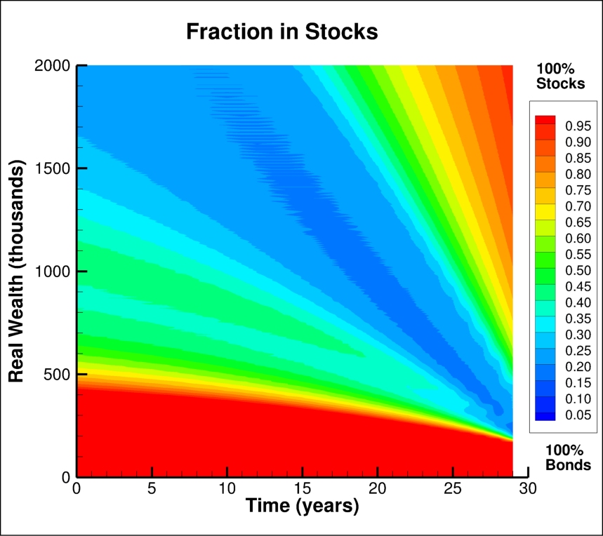
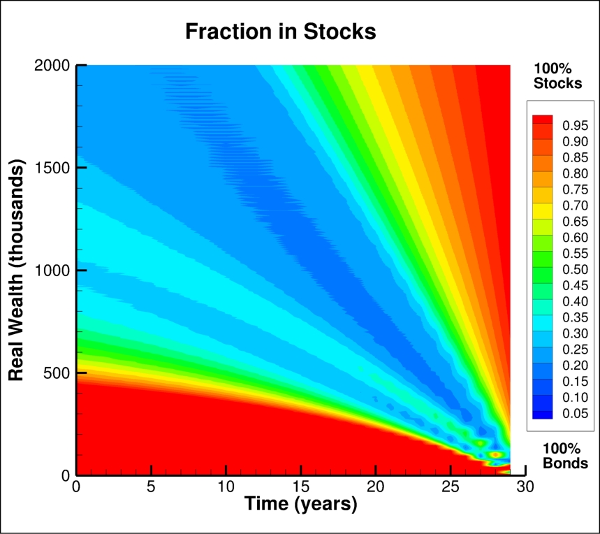
The percentiles of fraction in equities, wealth and withdrawals, for the point on the efficient frontier are shown in Figure 11.2, for the case . The heat maps of the controls for fraction in equities and optimal withdrawals are given in Figure 11.3. The normalized withdrawal is .
Note the interesting feature of the median withdrawal in Figure 2(c). The median withdrawal stays at for the first five years of retirement, then increases rapidly to by year seven. This is a result of the fact that the optimal withdrawal is very close to a bang-bang type control, as seen in the heat map shown in Figure 3(b). This is not unexpected, due the fact that in the continuous withdrawal/rebalancing limit, the withdrawal control (for a rate of withdrawals) is in fact bang-bang, as noted in Proposition 7.1.
The corresponding percentiles and heat maps for the case where are given in Figures 11.4 and 11.5, for the point on the EW-ES curve . These figures are qualitatively similar to the case.





12 Robustness check: historical market
We compute and store the optimal controls from Problem (5.2), and then use these controls in the bootstrapped historical market, as described in Section 9.2. Table B.1 shows the effect of using different blocksizes in the bootstrap simulations, compared to the synthetic market results. The expected withdrawals are all very close, for all blocksizes. There is more variability in the ES results, but this spread is acceptable for practical purposes. This indicates that the choice of blocksize will not influence the qualitative results appreciably. In the following, we will report results using a blocksize of years, which is justified from Table 9.2.
The detailed bootstrapped efficient frontiers (using the controls computed in the synthetic market) are given in Tables C.1 and C.2. In Figure 12.1, we compare the EW-ES frontiers computed for the case (i) controls computed in the synthetic market, frontier computed in the synthetic market and (ii) controls computed in the synthetic market, control tested in the historical market. We can see that the synthetic market frontiers are very close to the historical market frontiers. This indicates that the controls computed in the synthetic market are robust to uncertainty in the synthetic stochastic process model calibrated to historical data.
13 Discussion
Adding a variable withdrawal strategy, coupled with optimal asset allocation, can dramatically improve the expected average withdrawal, compared with a constant withdrawal strategy. If the minimum withdrawal of the variable strategy is set equal to the constant withdrawal strategy, then this result still holds, requiring only a small increase in risk, as measured by expected shortfall (ES).
At first sight, this result is almost too good to be true. However, this is easily explainable, due to two effects.
- •
The median final wealth of the variable withdrawal strategy is much lower than the constant withdrawal policy. Hence, the variable withdrawal strategy is much more efficient in disbursing cash to the retiree over the investment horizon, while keeping the overall risk almost unchanged.1010 10 “If we have a good year, we take a trip to China,…if we have a bad year, we stay home and play canasta.” retired professor Peter Ponzo, discussing his DC plan withdrawal strategy https://www.theglobeandmail.com/report-on-business/math-prof-tests-investing-formulas-strategies/article22397218/
- •
Due to the quasi-bang-bang control for the variable withdrawal strategy, the median optimal policy is to withdraw at the minimum rate for the first few years, followed by withdrawing at the maximum rate for 20-25 years. This avoids large withdrawals in the early years, ameliorating sequence of return risk, with the benefits to be gained in later years.
The downside of this strategy is that, although the average withdrawal is signficently improved, the first few years after retirement typically have the smallest (minimum) withdrawals. This may not be desirable, if retirees are most active at this time, and may wish to have larger incomes.
There are several ways to move spending earlier, but these all come at some cost in terms of EW-ES efficiency. Recall that all quantities in this paper are real, hence we are always preserving real spending power. However, we could add a real discounting multiplier to our measure of reward. This would change equation (4.4) to
| (13.1) |
where is a discounting parameter. We experimented with this approach, and it did tend to move more spending earlier, but at the expense of more risk. In fact, the results using a discounting factor were similar to simply decreasing the scalarization parameter in equation (5.1). The withdrawal control in this case was also quasi-bang-bang. Adding a discount factor does not change the bang-bang nature of the withdrawal control, at least in the continuous withdrawal limit. This can be be verified by adding a discounting factor to equation (7.6).
In order to produce a withdrawal control which is more gradual (not bang-bang), we need to add a nonlinearity to the measure of reward. Let be a utility function, then our measure of reward could be
| (13.2) |
We experimented with various utility functions (e.g. , power law), and this did have the effect of producing smoother controls as a function of wealth. However, this came at the cost of poor EW-ES efficiency. Recall that our initial objective in this work was to provide the retiree with fixed minimum cash flows, with small risk, while maximizing total withdrawals. Using a nonlinear utility function would conflict with this criteria. We leave exploration of the use of a nonlinear utility in the reward function as a topic for future work.
14 Conclusions
Our objective in this work was to provide a retiree with minimum fixed cash flows over a long time horizon, with high probability of expected average withdrawals being signficently larger than the minimum withdrawal. In addition, we control the risk of this strategy as measured by expected shortfall.
The optimal controls consisted of a variable withdrawal rate (with minimum and maximum constraints) and the asset allocation strategy. Allowing a variable withdrawal strategy (compared to a fixed withdrawal) dramatically improved the expected average withdrawals, at the expense of a very small increase in expected shortfall risk. However, the early withdrawals were (with high probability) at the minimum level, and larger withdrawals were achieved later on in life.
Note that the controls were computed in the synthetic market, i.e. a market based on a parametric stochastic process model calibrated to data over the 1926:1-2019:12 period. However, bootstrap resampling tests showed that this strategy is robust to model and parameter uncertainty.
An intriguing application of this research is the following. In many countries (Canada in particular), there is a reward, in terms of increased cash flows, if the retiree delays receiving government benefits, until later ages (e.g. 70 in Canada). The common advice is to delay receiving government benefits, and offset this with larger drawdowns from the DC account in the early years of retirement. The argument here is that government benefits are indexed and certain, compared with uncertain investment cash flows.
However, our results indicate that fairly small reductions in withdrawals from the DC account in early years result in much larger withdrawals in later years, with a high probability. Hence a better strategy may be to take some government benefits earlier, allowing smaller withdrawals from the DC account in early years (reducing sequence of return risk). The smaller government benefits in later years will (again, with high probability) be offset by these much larger withdrawals from the DC account. Of course, although this strategy has a high probability of success, it is not risk-free.
15 Acknowledgements
P. A. Forsyth’s work was supported by the Natural Sciences and Engineering Research Council of Canada (NSERC) grant RGPIN-2017-03760.
16 Conflicts of interest
The author has no conflicts of interest to report.
Appendix
Appendix A Detailed efficient frontiers: synthetic market
| ES (5%) | ||||
|---|---|---|---|---|
| 0.05 | -498.2 | 56.83 | 119.7 | .430 |
| 0.2 | -177.9 | 53.24 | 324.9 | .405 |
| 0.5 | -50.86 | 51.33 | 368.2 | .363 |
| 1.0 | -4.730 | 49.89 | 406.3 | .331 |
| 5.0 | 25.79 | 47.67 | 451.8 | .282 |
| 50.0 | 30.62 | 45.63 | 524.6 | .259 |
| 5000.0 | 31.02 | 42.90 | 661.8 | .252 |
| ES (5%) | ||||
|---|---|---|---|---|
| 0.1 | -587.3 | 59.98 | 46.36 | .455 |
| 0.5 | -260.8 | 55.97 | 75.06 | .418 |
| 1.0 | -237.2 | 55.00 | 73.61 | .366 |
| 1.75 | -209.5 | 54.32 | 75.49 | .341 |
| 2.5 | - 204.7 | 53.95 | 78.56 | .331 |
| 5.0 | -199.8 | 53.44 | 78.31 | .314 |
| 10.0 | -197.8 | 52.98 | 91.68 | .303 |
| -196.2 | 50.63 | 202.1 | .285 | |
| -196.1 | 48.91 | 316.0 | .303 |
Appendix B Effect of blocksize: stationary block bootstrap resampling
Table B.1 shows the effect of blocksize on the bootstrap resampling algorithm.
| ES (5%) | ||||
|---|---|---|---|---|
| Synthetic Market | ||||
| 0.5 | -50.86 | 51.33 | 368.2 | .363 |
| Historical Market: years. | ||||
| -17.28 | 51.19 | 340.6 | .360 | |
| Historical Market: years. | ||||
| -40.63 | 51.19 | 343.1 | .361 | |
| Historical Market: years. | ||||
| -34.13 | 51.23 | 342.9 | .361 | |
| Synthetic Market | ||||
| 1.0 | 4.730 | 49.89 | 406.3 | .331 |
| Historical Market: years. | ||||
| 20.47 | 49.72 | 381.0 | .330 | |
| Historical Market: years. | ||||
| -5.10 | 49.72 | 383.6 | .331 | |
| Historical Market: years. | ||||
| -0.84 | 49.74 | 384.4 | .331 | |
Appendix C Bootstrapped frontiers
Tables C.1 and C.2 show the detailed results for the EW-ES frontiers. The controls were computed in the synthetic market, and tested in the historical market.
| ES (5%) | ||||
| 0.05 | -450.9 | 56.84 | 90.31 | .424 |
| 0.2 | -126.7 | 53.16 | 294.7 | .402 |
| 0.5 | -17.28 | 51.20 | 340.6 | .360 |
| 1.0 | 20.47 | 49.72 | 381.0 | .330 |
| 5.0 | 42.86 | 47.45 | 430.3 | .282 |
| 50.0 | 45.39 | 45.38 | 502.5 | .258 |
| 5000.0 | 45.64 | 42.62 | 638.9 | .252 |
| N/A | 45.63 | 35.0 | 920.0 | .269 |
| ES (5%) | ||||
|---|---|---|---|---|
| 0.1 | -531.8 | 59.94 | 25.99 | .453 |
| 0.5 | -230.3 | 55.83 | 53.89 | .412 |
| 1.0 | -202.2 | 54.84 | 54.30 | .363 |
| 1.75 | -192.3 | 54.14 | 57.13 | .337 |
| 5.0 | -185.8 | 53.24 | 61.79 | .310 |
| 10.0 | -184.3 | 52.69 | 75.40 | .299 |
| 1000.0 | -183.5 | 50.43 | 186.3 | .283 |
| -183.5 | 48.69 | 296.9 | .300 | |
| N/A | -183.5 | 40.0 | 676.7 | .340 |
References
- Bengen (1994) Bengen, W. (1994). Determining withdrawal rates using historical data. Journal of Financial Planning 7, 171–180.
- Bernhardt and Donnelly (2018) Bernhardt, T. and C. Donnelly (2018). Pension decumulation strategies: A state of the art report. Technical Report, Risk Insight Lab, Heriot Watt University.
- Cont and Mancini (2011) Cont, R. and C. Mancini (2011). Nonparametric tests for pathwise properties of semimartingales. Bernoulli 17, 781–813.
- Dang and Forsyth (2014) Dang, D.-M. and P. A. Forsyth (2014). Continuous time mean-variance optimal portfolio allocation under jump diffusion: a numerical impulse control approach. Numerical Methods for Partial Differential Equations 30, 664–698.
- Dang and Forsyth (2016) Dang, D.-M. and P. A. Forsyth (2016). Better than pre-commitment mean-variance portfolio allocation strategies: a semi-self-financing Hamilton-Jacobi-Bellman equation approach. European Journal of Operational Research 250, 827–841.
- Dichtl et al. (2016) Dichtl, H., W. Drobetz, and M. Wambach (2016). Testing rebalancing strategies for stock-bond portfolos across different asset allocations. Applied Economics 48, 772–788.
- Forsyth and Labahn (2019) Forsyth, P. and G. Labahn (2019). Monotone Fourier methods for optimal stochastic control in finance. Journal of Computational Finance 22:4, 25–71.
- Forsyth (2020a) Forsyth, P. A. (2020a). Multi-period mean CVAR asset allocation: Is it advantageous to be time consistent? SIAM Journal on Financial Mathematics 11:2, 358–384.
- Forsyth (2020b) Forsyth, P. A. (2020b). Optimal dynamic asset allocation for DC plan accumulation/decumulation: Ambition-CVAR. Insurance: Mathematics and Economics 93, 230–245.
- Forsyth and Vetzal (2019) Forsyth, P. A. and K. R. Vetzal (2019). Optimal asset allocation for retirement savings: deterministic vs. time consistent adaptive strategies. Applied Mathematical Finance 26:1, 1–37.
- Forsyth et al. (2019) Forsyth, P. A., K. R. Vetzal, and G. Westmacott (2019). Management of portfolio depletion risk through optimal life cycle asset allocation. North American Actuarial Journal 23:3, 447–468.
- Forsyth et al. (2020) Forsyth, P. A., K. R. Vetzal, and G. Westmacott (2020). Optimal asset allocation for a DC pension decumulation with a variable spending rule. ASTIN Bulletin 50:2, 419–447.
- Homer and Sylla (2005) Homer, S. and R. Sylla (2005). A History of Interest Rates. New York: Wiley.
- Kou (2002) Kou, S. G. (2002). A jump-diffusion model for option pricing. Management Science 48, 1086–1101.
- Kou and Wang (2004) Kou, S. G. and H. Wang (2004). Option pricing under a double exponential jump diffusion model. Management Science 50, 1178–1192.
- Lin et al. (2015) Lin, Y., R. MacMinn, and R. Tian (2015). De-risking defined benefit plans. Insurance: Mathematics and Economics 63, 52–65.
- Ma and Forsyth (2016) Ma, K. and P. A. Forsyth (2016). Numerical solution of the Hamilton-Jacobi-Bellman formulation for continuous time mean variance asset allocation under stochastic volatility. Journal of Computational Finance 20(1), 1–37.
- MacDonald et al. (2013) MacDonald, B.-J., B. Jones, R. J. Morrison, R. L. Brown, and M. Hardy (2013). Research and reality: A literature review on drawing down retirement financial savings. North American Actuarial Journal 17, 181–215.
- MacMinn et al. (2014) MacMinn, R., P. Brockett, J. Wang, Y. Lin, and R. Tian (2014). The securitization of longevity risk and its implications for retirement security. In O. S. Mitchell, R. Maurer, and P. B. Hammond (Eds.), Recreating Sustainable Retirement, pp. 134–160. Oxford: Oxford University Press.
- Mancini (2009) Mancini, C. (2009). Non-parametric threshold estimation models with stochastic diffusion coefficient and jumps. Scandinavian Journal of Statistics 36, 270–296.
- Menoncin and Vigna (2017) Menoncin, F. and E. Vigna (2017). Mean-variance target based optimisation for defined contribution pension schemes in a stochastic framework. Insurance: Mathematics and Economics 76, 172–184.
- Patton et al. (2009) Patton, A., D. Politis, and H. White (2009). Correction to: automatic block-length selection for the dependent bootstrap. Econometric Reviews 28, 372–375.
- Peijnenburg et al. (2016) Peijnenburg, K., T. Nijman, and B. J. Werker (2016). The annuity puzzle remains a puzzle. Journal of Economic Dynamics and Control 70, 18–35.
- Politis and Romano (1994) Politis, D. and J. Romano (1994). The stationary bootstrap. Journal of the American Statistical Association 89, 1303–1313.
- Politis and White (2004) Politis, D. and H. White (2004). Automatic block-length selection for the dependent bootstrap. Econometric Reviews 23, 53–70.
- Ritholz (2017) Ritholz, B. (2017). Tackling the ‘nastiest, hardest problem in finance’. www.bloomberg.com/view/articles/2017-06-05/tackling-the-nastiest-hardest-problem-in-finance.
- Rockafellar and Uryasev (2000) Rockafellar, R. T. and S. Uryasev (2000). Optimization of conditional value-at-risk. Journal of Risk 2, 21–42.
- Staden et al. (2018) Staden, P. V., D.-M. Dang, and P. Forsyth (2018). Time-consistent mean-variance portfolio optimization: a numerical impulse control approach. Insurance: Mathematics and Economics 83, 9–28.
- Strub et al. (2019) Strub, M., D. Li, and X. Cui (2019). An enhanced mean-variance framework for robo-advising applications. SSRN 3302111.
- Tankov and Cont (2009) Tankov, P. and R. Cont (2009). Financial Modelling with Jump Processes. New York: Chapman and Hall/CRC.
- Towers-Watson (2020) Towers-Watson (2020). The global pension assets study 2020. https://www.thinkingaheadinstitute.org/en/Library/Public/Research-and-Ideas/2020/01/Global-Pension-Asset-Study-2020.
- Tretiakova and Yamada (2011) Tretiakova, I. and M. S. Yamada (2011). What DC plan members really want. Rotman International Journal of Pension Managment 4:2, 60–70.
- Vigna (2014) Vigna, E. (2014). On efficiency of mean-variance based portfolio selection in defined contribution pension schemes. Quantitative Finance 14, 237–258.
- Waring and Siegel (2015) Waring, M. B. and L. B. Siegel (2015). The only spending rule article you will ever need. Financial Analysts Journal 71(1), 91–107.
- Westmacott and Daley (2015) Westmacott, G. and S. Daley (2015). The design and depletion of retirement portfolios. PWL Capital White Paper.