Learning Lyapunov Functions for Piecewise Affine Systems with Neural Network Controllers
Abstract
We propose a learning-based method for Lyapunov stability analysis of piecewise affine dynamical systems in feedback with piecewise affine neural network controllers. The proposed method consists of an iterative interaction between a learner and a verifier, where in each iteration, the learner uses a collection of samples of the closed-loop system to propose a Lyapunov function candidate as the solution to a convex program. The learner then queries the verifier, which solves a mixed-integer program to either validate the proposed Lyapunov function candidate or reject it with a counterexample, i.e., a state where the stability condition fails. This counterexample is then added to the sample set of the learner to refine the set of Lyapunov function candidates. We design the learner and the verifier based on the analytic center cutting-plane method, in which the verifier acts as the cutting-plane oracle to refine the set of Lyapunov function candidates. We show that when the set of Lyapunov functions is full-dimensional in the parameter space, the overall procedure finds a Lyapunov function in a finite number of iterations. We demonstrate the utility of the proposed method in searching for quadratic and piecewise quadratic Lyapunov functions.
1 Introduction
Deep neural networks (DNNs) have achieved remarkable success in various challenging tasks across different fields such as image classification [1], machine translation [2], speech recognition [3], reinforcement learning, and control [4]. The high performance of DNNs, however, does not come with guarantees as they are highly complex and, therefore, hard to reason about. Moreover, it is relatively well-known that neural networks can be sensitive to input perturbations and adversarial attacks [5, 6]. These drawbacks limit the application of DNNs in safety-critical systems, in which standard control strategies, although potentially inferior to DNNs in performance, do have performance guarantees. Therefore, it is critical to develop tools that can provide useful certificates of stability, safety, and robustness for DNN-driven systems.
Stability analysis aims to show that a set of initial states of a dynamical system would stay around and potentially converge to an equilibrium point. Stability analysis of dynamical systems often relies on constructing Lyapunov functions that can find positive invariant sets, certify the stability of equilibrium points, and estimate their region of attraction. Finding non-conservative Lyapunov functions for generic nonlinear systems, however, is not an easy task and often requires substantial expertise, manual effort, and expensive numerics in the form of complex optimization problems. This task becomes even more challenging when neural networks (NNs) are used as stabilizing controllers. In this context, it is of great interest to automate the construction of Lyapunov functions for various classes of nonlinear systems [7] and, in particular, neural-network-controlled feedback systems.
The complexity of finding Lyapunov functions for nonlinear systems has also motivated the use of data-driven methods, which aim at “learning” Lyapunov functions from observations or simulation traces. The intuition is that a Lyapunov function constructed from finitely many trajectories would hopefully be a valid Lyapunov function for all possible trajectories. Although these methods do not require a model of the system to be available, they generally rely on a large number of simulations and often lack formal guarantees despite the high confidence gained from many simulations.
Contributions: We propose a sample-efficient optimization-based method to synthesize Lyapunov functions for discrete-time piecewise affine systems in feedback with ReLU neural network controllers. The proposed algorithm relies on a “learner”, which proposes a Lyapunov function candidate using finitely many samples, and a “verifier”, which either validates the Lyapunov function candidate or rejects it with a counterexample, i.e., a state where the stability condition fails. This counterexample is then added to the sample set of the learner to refine the set of Lyapunov function candidates. We design the learner and the verifier according to the analytic center cutting-plane method (ACCPM) from convex optimization, with which the algorithm can efficiently and exhaustively search over the considered Lyapunov function candidate class. Notably, the algorithm is guaranteed to terminate in finite steps if the set of Lyapunov function is full-dimensional in the parameter space. We demonstrate the application of our algorithm to search for quadratic and piecewise quadratic Lyapunov functions.
1.1 Related work
Output range analysis of NNs: Driven by the need to verify the robustness of deep neural networks against adversarial attacks [5], a large body of work has been reported on bounding the output of DNNs for a given range of inputs [8, 9, 10, 11, 12, 13, 14]. These methods can be categorized into exact or approximate depending on how they evaluate/approximate the nonlinear activation functions in the DNN. Of particular interest to this paper is the tight certification of ReLU NNs through formal verification techniques such as Satisfiability Modulo Theories (SMT) solvers [12, 14, 15] or mixed-integer programming (MIP) [9, 16]. These approaches can verify the linear properties of the ReLU NN output given linear constraints on the network inputs. More scalable but less accurate methods that apply linear programming (LP) [10] or semidefinite programming (SDP) relaxations [11, 13, 17, 18] of NNs to over approximate the output range can be found in the literature.
Stability and reachability analysis of NN-controlled systems: Despite their high performance, NN-controlled systems lack safety and stability guarantees. Motivated by this, several works have studied the challenging task of verifying NN-controlled systems. In [19], built upon the framework of [11], the authors over-approximate the reachable set of NN-controlled LTI systems by bounding the nonlinear activation functions of the NN through quadratic constraints (QCs). In [20, 21], the authors approximate NN functions through polynomial approximations to conduct a closed-loop reachability analysis. Ivanov et al. [22] transform a sigmoid-based NN into a hybrid system and propose the verification of the NN-controlled system through standard hybrid system verification tools.
For stability analysis, linear matrix inequality (LMI)-based sufficient stability conditions are derived by abstracting the nonlinear activation function in NNs through QCs [23] or by linear difference inclusions [24, 25]. Yin et al. [26] use a QC abstraction of NNs to analyze uncertain plants with perturbations described by integral quadratic constraints (IQCs). The input-output stability of an NN-controlled system is considered in [27] where QCs are constructed from the bounds of partial gradients of NN controllers. For ReLU NN controllers, the authors in [28] exploit the fact that a ReLU NN induces a piecewise affine (PWA) function and analyze the closed-loop stability by identifying the linear dynamics around the equilibrium. However, the number of modes generated by the ReLU NN is exponential in the number of neurons, and can easily make general PWA system stability analysis tools intractable [29, 30, 31, 32].
Stability analysis of PWA systems: In this paper, we consider PWA systems in feedback with ReLU NN controllers. The closed-loop system is itself an autonomous PWA system since a ReLU NN is, in fact, a continuous PWA function [33]. For continuous-time PWA systems, LMI-based approaches to synthesize piecewise affine [34], piecewise quadratic (PWQ) [31] and piecewise polynomial Lyapunov functions [35] have been proposed. The adaptation of these Lyapunov function synthesis methods for discrete-time PWA systems is summarized in [29].
Although formulated as convex programs, these methods require parameterizing a Lyapunov function candidate on each mode, and identifying the pairwise one-step transition sets between the modes for discrete-time PWA systems. Since the number of partitions generated by a deep ReLU network can be extremely large [33], the aforementioned methods involve solving large-scale convex problems. Taking PWQ Lyapunov function synthesis as an example, the approach proposed in [29] requires solving a large-scale SDP which is conservative and only provides a sufficient condition for stability due to the application of the -procedure [36]. In this paper, we propose an MIP-based iterative approach for quadratic and PWQ Lyapunov function synthesis for a discrete-time PWA system controlled by a ReLU NN controller. Our proposed method does not require identifying all the partitions of the ReLU network and is non-conservative.
Sample-based Lyapunov function synthesis: Synthesizing Lyapunov functions for nonlinear dynamical systems is very difficult, in general, and often involves solving large, nonconvex optimization problems. To avoid solving hard optimization problems directly, several sample-based Lyapunov function synthesis methods have been proposed. Topcu et al. [37] use simulation data to help postulate the region of attraction of continuous-time polynomial systems and find Lyapunov function candidates for solving bilinear matrix inequalities. Boffi et al. [38] propose a data-driven method that can learn Lyapunov functions from system trajectory data with probabilistic guarantees. Closely related to our work is [39], where an iterative approach formulates Lyapunov function candidates for continuous-time nonlinear systems from simulation traces and improves the result by the counterexample trace generated by a falsifier at each iteration. Our method differs from theirs in that we provide a finite-step termination guarantee for our iterative algorithm.
Counterexample guided inductive synthesis: The iterative approach alternating between a learning module and a verification module to synthesize a certificate for control systems is known as the Counter-Example Guided Inductive Synthesis (CEGIS) framework proposed by [40, 41] in the verification community. The application of CEGIS on Lyapunov function synthesis for continuous-time nonlinear autonomous systems can be found in [42, 7] using SMT solvers for verification. However, the termination of the iterative procedures in these works is not guaranteed. Notably, Ravanbakhsh et al. [43] apply the CEGIS framework to synthesize control Lyapunov functions for nonlinear continuous-time systems and provide finite-step termination guarantees for the iterative algorithm through careful design of the learner, which essentially implements the maximum volume ellipsoid cutting-plane method [44]. Although our method also provides termination guarantees through the (analytic center) cutting-plane method, the considered problem setting (stability verification of NN-controlled PWA system), and the construction of the learner and the verifier are highly different.
The rest of the paper is organized as follows. After introducing the preliminaries on Lyapunov functions in Section 2, we state our problem formulation as finding an estimate of the region of attraction of a NN-controlled PWA system in Section 3. We develop our method in Section 4 and discuss its extensions and variations in Section 5. Section 6 demonstrates the application of the proposed method through numerical examples and Section 7 concludes the paper.
1.2 Notations
We denote the set of real numbers by , the set of integers by , the -dimensional real vector space by , and the set of real matrices by . The standard inner product between two matrices is given by and the Frobenius norm of a matrix is given by . We denote the set of symmetric matrices by , and (resp., ) denotes the set of positive semidefinite (resp., definite) matrices. For two vectors and , represents their concatenation. Given a set denotes the orthogonal projection of onto the subspace . Given a point and a compact set , define the projection of to the set as where is the Euclidean norm of . For a set , we denote the closure of , the set of all interior points in , and the recession cone of .
2 Preliminaries
2.1 Stability of nonlinear autonomous systems
Consider a discrete-time autonomous system
| (1) |
where is the state and is a nonlinear, continuous function with domain . Without loss of generality, we assume is an equilibrium of the system, i.e., . Denote the state of system (1) at time and the initial state. To study the stability properties of autonomous systems at their equilibrium points, Lyapunov functions may be used.
Definition 1.
(Lyapunov stability [45, Chapter 13]) The equilibrium point of the autonomous system (1) is
- •
Lyapunov stable if for each , there exists such that if , then .
- •
asymptotically stable if it is Lyapunov stable and there exists such that if , then .
- •
geometrically stable if there exists such that if , then .
For an asymptotically stable equilibrium point, the region of attraction (ROA) is the set of initial states from which the trajectories of the autonomous system converge to the equilibrium.
Definition 2 (Region of attraction).
The ROA of the autonomous system (1) is defined as
Definition 3 (Successor set).
For the autonomous system (1), we denote the successor set from a set as .
Definition 4 (Positive invariant set).
A set is said to be positive invariant for the autonomous system (1) if for all , we have .
Theorem 1.
([45, Chapter 13]) Consider the discrete-time nonlinear system (1) and assume there is a continuous function with domain such that
| (2a) | ||||
| (2b) | ||||
where the set is the region of interest (ROI) satisfying , , and . Then the origin is Lyapunov stable. If, in addition,
| (3) |
then the origin is asymptotically stable.
We call any satisfying the condition (2a) a Lyapunov function candidate. If additionally, satisfies the condition (2b) or (3), then is called a valid Lyapunov function candidate. Since asymptotic stability is our primary focus in this paper, a Lyapunov function is any satisfying constraints (2a) and (3) unless specified otherwise. Let . Then the set
| (4) |
is an inner approximation of the ROA and is the largest sublevel set of that is contained in .
3 Problem Statement
3.1 Plant model
In this paper, we consider discrete-time piecewise affine (PWA) dynamical systems of the form
| (5) |
where is the state, is the control input, denotes the state at the next time instant, is the mode of the system, and are polytopic partitions (i.e., is a bounded polyhedron) of the domain . We assume that the partitions satisfy and the PWA dynamics (5) is well-posed, i.e., . We denote the PWA system (5) compactly as . Without loss of generality, we assume the origin is an equilibrium point of the PWA system, i.e., . As a special case, the PWA system (5) reduces to a linear time-invariant (LTI) system when there is only one mode. In this case, we denote the LTI system as
| (6) |
3.2 Neural network controller model
In this paper we assume the PWA dynamical system (5) is driven by a multi-layer piecewise linear neural network controller , where is described by
| (7) | ||||
Here, is the input to the neural network, is the vector representing the output of the -th hidden layer with neurons, is the output of the neural network, and are the weight matrix and the bias vector of the -th hidden layer.
3.3 Closed-loop stability analysis
We denote the closed-loop dynamics of the PWA system (5) in feedback with the ReLU network controller (7) as
| (8) |
Under the assumption , the origin is an equilibrium of the closed-loop system, i.e., . Define the region of interest as a polytopic set given by
| (9) |
We are interested in verifying the stability of the equilibrium point and finding an inner estimate of its ROA contained in , where the ROI can be interpreted as a user-defined set that guides the search for an estimate of the ROA.
Problem 1.
Find an inner estimate of the ROA, , for the closed-loop system (8).

4 Learning Lyapunov functions for the closed-loop system
To solve Problem 1, we propose an iterative learning-based method to construct a valid Lyapunov function for the closed-loop system (8). In each iteration of this algorithm, a “learner” proposes a Lyapunov function candidate using a collection of samples of the closed-loop system. The learner then queries a “verifier” that either certifies that the proposed function is a valid Lyapunov function or rejects it with a counterexample, i.e., a state where the stability condition fails. This counterexample is then added to the training set of the learner. In the next iteration, the learner uses the new counterexample and a cutting-plane strategy to refine the set of Lyapunov function candidates. The learner repeats this process until termination when either it finds a valid Lyapunov function, or it verifies its non-existence in the given parameterized function space. In our framework, the learner solves a convex optimization problem to synthesize Lyapunov function candidates, and the verifier solves a mixed-integer program (MIP) to generate the counterexamples. We provide a finite-step termination guarantee for our algorithm through the analysis of cutting-plane methods from convex optimization. The proposed method is illustrated in Fig. 2.

4.1 Quadratic Lyapunov functions
We begin by considering a quadratic Lyapunov function candidate of the form
| (10) |
with the matrix parameter and domain the same as that of the PWA system (5). We aim to find a such that would satisfy the constraint (3). Since we can always scale while satisfying constraint (3), without loss of generality, we describe the set of valid Lyapunov function candidate parameters as
| (11) |
We observe that is a convex set defined by semidefinite constraints and infinitely many linear constraints on . Although, theoretically, a feasible point in can be obtained by solving a convex semi-infinite feasibility problem [46], such an approach is numerically intractable. This motivates sample-based approaches which instead require the constraints in (11) to only hold for a finite set of samples , resulting in an over-approximation 11 1 For numerical reasons, we define the over-approximation of as a compact set. As will be shown in the following sections, our proposed method will find a feasible point in the interior of the closure of using barrier functions. Therefore, if is non-empty, our method will find a feasible point in satisfying all the strict inequalities. of :
| (12) |
Finding a feasible point in is now a tractable convex feasibility program. However, there is no guarantee that the resulting solution would correspond to a valid Lyapunov function candidate, even if the number of samples approaches infinity. In this paper, we propose an efficient sampling strategy based on the analytic center cutting-plane method (ACCPM) to iteratively grow the sample set and refine the set until we find a feasible point in . In the next subsections, we describe the proposed approach and provide finite-step termination and validity guarantees.
4.2 The analytic center cutting-plane method
Cutting-plane methods [47, 48, 49] are iterative algorithms to find a point in a target convex set or to determine whether is empty. In these methods, we have no information of except for a “cutting-plane oracle” described below. At each iteration , we have a “localization” set defined by a finite set of inequalities that over-approximates the target set, i.e., . If is empty, then we have a proof that the target set is also empty. Otherwise, we query the oracle at a point . If , the oracle returns ‘yes’ and the algorithm terminates; if , it returns ‘no’ together with a separating hyperplane that separates and . In the latter case, the cutting-plane method updates the localization set by (see Fig. 3). This process continues until either a point in the target set is found or the target set is certified to be empty.
Based on how the query point is chosen, different cutting-plane methods have been proposed including the center of gravity method [50], the maximum volume ellipsoid (MVE) cutting-plane method [44], the Chebyshev center cutting-plane method [48], the ellipsoid method [51, 52], the volumetric center cutting-plane method [53], and the analytic center cutting-plane method [54, 55, 47]. In this paper, the query point is chosen as the analytic center of according to the ACCPM, since it allows the localization set to be described by linear matrix inequalities.

Definition 5 (Analytic center [56]).
The analytic center of the set , is defined as the optimal solution of the convex problem
| (13) |
To implement the ACCPM, we introduce a learner, which proposes Lyapunov function candidates based on a set of samples, and a verifier, which serves as a cutting-plane oracle. We describe each one of these two elements below.
4.3 The learner
Let be a collection of samples from . The step-wise increment in the Lyapunov function as a function of the current state and the matrix can be written as
which is a linear function in . Based on the sample set , we construct an outer-approximation of as
| (14) |
The localization set represents the learner’s knowledge about by observing the one-step state transitions of the dynamical system from the sample set . Utilizing the ACCPM, the learner proposes a Lyapunov function candidate with as the analytic center of :
| (15) |
We denote the objective function in (15) as and call it the potential function of the set . If (15) is infeasible, then we have a proof that no quadratic Lyapunov function exists for the closed-loop system. Otherwise, the learner proposes as a Lyapunov function candidate. Due to the log-barrier function in (15), is in the interior of . At initialization, we have an empty sample set, i.e., and the potential function simply becomes with as the analytic center.
4.4 The verifier
Given a Lyapunov function candidate proposed by the learner at iteration , the verifier either ensures that this function satisfies the constraints in (2a) and (3), or returns a state where constraint (2a) or (3) is violated as a counterexample. Since the log-barrier function in (15) guarantees , constraint (2a) is readily satisfied and the verifier must check the violation of constraint (3). This can be done by solving the optimization problem
| (16) |
Next, we will show that for PWA systems and ReLU NN controllers, the optimization problem (16) can be formulated as a mixed-integer quadratic program (MIQP). This is based on the fact that both the PWA dynamics and the ReLU NN controller can be described by a set of mixed-integer linear constraints.
4.4.1 Mixed-integer formulation of PWA dynamics
To formulate optimization problems involving hybrid dynamics, e.g., the optimal control problem of PWA systems, we need to describe system (5) in a form compatible with optimization solvers. In this paper, we use disjunctive programming [57] to describe the PWA dynamics (5), which exploits the underlying geometry of the system. Other modeling approaches, e.g., mixed logical dynamical (MLD) formulation [58], are also applicable and our proposed method can be easily extended to these modeling approaches since all of them encode the PWA dynamics by mixed-integer linear constraints.
Recall that the PWA dynamics (5) is given by if . Equivalently, we can describe the PWA dynamics in in the lifted space of as , where is the graph of which is defined as the following polytope in :
| (17) |
The first two block rows of and define the dynamics and the third block row constrains to lie in . In the last block row, we add an artificial constraint on the control input, where is a bounded set in . This guarantees that have a common recession cone for all . Details of choosing will be discussed in Section 4.5. Following from the definition of , we have
By denoting the PWA dynamics collectively as , we define the graph of as . Then we have
which indicates that the evolution of the PWA dynamics is constrained in a union of disjunctive sets . As a result, optimization over subject to the PWA system dynamics is equivalent to optimizing over the set . Next, we will show that lends itself to a mixed-integer formulation.
Definition 6 (Mixed-integer formulation of a set [57]).
For a set , consider the set in a lifted space given by
| (18) |
with a function and a vector . The set is a mixed-integer formulation of if . If the function is linear (convex), we call the related formulation MIL (MIC).
In Definition 6, if has a mixed-integer formulation , then can be represented by the inequalities , which means
For the PWA dynamics , we construct an MIL formulation of , known as the convex-hull formulation [57], in the following lemma.
Lemma 1.
For PWA system defined in (5), let for . Then the set defined by the constraints
| (19) | ||||
is an MIL formulation of .
Proof.
Since and are bounded, share the common recession cone for all . By [57, Corollary ], the set in the lemma is an MIL formulation of . ∎
In constraints (19), the binary variable can be interpreted as an indicator of the current mode of the state . For instance, let and consequently . Since , we have . Then the state satisfies , i.e., . Similarly, and . It then follows . The MIL formulation of in (19) allows us to represent the PWA dynamical constraint through a finite number of mixed-integer linear constraints.
4.4.2 Mixed-integer formulation of ReLU NN
Consider a scalar ReLU function where . Then it can be shown that the ReLU function admits the following mixed-integer representation [16],
| (20) |
where the binary variable is an indicator of the activation function being active () or inactive (). Now consider a ReLU network described by the equations in (7). Suppose and are known element-wise lower and upper bounds on the input to the -th activation layer, i.e., . Then the neural network equations are equivalent to a set of mixed-integer constraints:
| (21) |
where is a vector of binary variables for the -th activation layer and denotes the vector of all ones. We note that the element-wise pre-activation bounds can be found by, for example, interval bound propagation or linear programming assuming known bounds on the input of the neural network [59, 60, 61, 62, 10]. Since state-of-the-art solvers for mixed-integer programming are based on the BranchBound algorithm [63], tight upper/lower bounds will allow the BranchBound algorithm to prune branches more efficiently and reduce the total running time.
4.4.3 Verifier construction through MIQP
Having the mixed-integer formulation of the PWA dynamics and the ReLU network at our disposal, we can formulate the verifier’s optimization problem (16) as the following MIQP:
| (22a) | ||||
| (22b) | ||||
| (22c) | ||||
| (22d) | ||||
| (22e) | ||||
| (22f) | ||||
| (22g) | ||||
| (22h) | ||||
| (22i) | ||||
| (22j) | ||||
| (22k) | ||||
| (22l) | ||||
| (22m) | ||||
Constraint (22b) restricts the search space to ; constraint (22c) with excludes a neighborhood around the origin22 2 For choice of see the discussion in Section 4.5. to verify constraint (3) with strict inequalities; constraints (22d) to (22i) exactly model the ReLU network controller with known layer-wise upper and lower bounds (see Section 4.4.2); and constraints (22j) to (22m) describe the PWA dynamics (see Section 4.4.1). The objective function (22a) aims to find a counterexample where the Lyapunov condition (3) is violated with the largest margin.
Denote by the optimal solution and the optimal value of problem (22). If , then we have a proof that is a Lyapunov function, since for all where and we terminate the search. As will be shown in Section 4.5, the choice of guarantees is sufficient to prove the asymptotic stability of the origin. If , then we reject the Lyapunov function candidate with as the counterexample since constraint (3) is violated at a non-zero state with . Meanwhile, we obtain a separating hyperplane in such that for all . Therefore, the MIQP (22) serves as a cutting-plane oracle.
4.5 Implementation of the ACCPM
With a learner that solves the convex program in (15) and a verifier that solves the MIQP in (22), we summarize the overall procedure in Algorithm 1. In Algorithm 1, we iteratively grow the sample set through the interaction between the learner and the verifier to guide the search for Lyapunov functions. Several practical issues of implementing Algorithm 1 are addressed below.
Input: initial sample set
Output:
, Status
Exclusion of the origin: In the MIQP (22), we exclude the -norm ball in order to verify asymptotic stability of the origin. The choice of is based on the observation that the closed-loop system is actually a PWA autonomous system and we can identify the local linear dynamics in the polytopic partition that contains the origin [28]. It follows from linear system theory that the origin is asymptotically stable if and only if all eigenvalues of have magnitudes less than [64]. As a result, we choose small enough such that and divide the asymptotic stability verification into two steps: use MIQP (22) to show the convergence of closed-loop trajectories to and use to prove the convergence to the origin. Since the stability of can be easily verified, our goal is to find a Lyapunov function that certifies the convergence of closed-loop trajectories to .
Solvability of nonconvex MIQP: The optimization problem (22) is a nonconvex MIQP since the quadratic objective function (22a) is indefinite. Therefore, the relaxation of the problem after removing the integer constraints would result in a nonconvex quadratic program. Nonconvex MIQP can be solved to global optimality through Gurobi v [65] by transforming the nonconvex quadratic expression into a bilinear form and applying spatial branching [66]. More information on solving nonconvex mixed-integer nonlinear programming can be found in [67, 68, 69]. In this paper, we rely on Gurobi to solve the nonconvex MIQP (22) automatically.
Choice of upper/lower bounds : As discussed in Section 4.4.2, tight element-wise upper and lowers bounds on the pre-activation values would lead to a more efficient pruning in the BranchBound algorithm and consequently reduce the overall running time. Finding tighter bounds, however, would require more computation. This trade-off has been explored in the context of neural network verification in [16].
Choice of artificial control input constraint: In the definition of , we introduced the artificial control input constraint . First, should be a bounded set to guarantee the validity of (19). Second, should be an over-approximation of the output range of over to guarantee that the MIQP (22) searches over all . This can be done by choosing as a box constraint and applying interval arithmetic [70] to over-approximate the output range of . Other output range analysis tools based on LP [10], SDP [11, 13], or MILP [16] are also applicable.
Normalization of the separating hyperplane: Let . When generating the localization set , we apply the linear constraint for all where . We normalize the linear constraint by and use the normalized constraint in the analytic center optimization problem (15).
Next, we provide finite-step termination guarantees for the proposed algorithm based on the analysis of the ACCPM from convex optimization.
4.6 Convergence analysis
The convergence and complexity of the ACCPM have been studied in [47, 55, 71, 72, 73, 74] under various assumptions on the localization set, the form of the separating hyperplane, whether multiple cuts are applied, etc. Directly related to Algorithm 1 and the search for a quadratic Lyapunov function is [74], which analyzes the complexity of the ACCPM with a matrix variable and semidefiniteness constraints. Notably, it provides an upper bound on the number of iterations that Algorithm 1 can run before termination. In [74], it is assumed that
- •
A1: is a convex subset of .
- •
A2: contains a non-degenerate ball of radius , i.e., there exists such that where is the Frobenius norm.
- •
A3: .
Let the ACCPM start with the localization set (or empty sample set in (15)) and initialize the first query point correspondingly. If at iteration , a query point is rejected by the oracle, a separating hyperplane of the form is given and is normalized to satisfy . Then by induction, each localization set with is given by
with defining the separating hyperplane at iteration and . The analytic center of is found by minimizing its potential function
| (23) |
i.e., the query point at iteration . Then the ACCPM following the above description achieves the following finite-step termination guarantee.
Theorem 2.
The analytic center cutting-plane method under assumptions A1 to A3 terminates in at most calls to the oracle.
Proof.
Sketch of proof: For the sequence of localization sets , [74] computes an upper bound on the potential function which is approximately , and a lower bound on which is proportional to . Since the ACCPM must terminate before the lower bound exceeds the upper bound, we obtain the finite-step termination guarantee in Theorem 2. ∎
The application of Theorem 2 to Algorithm 1 is direct. In Algorithm 1, we choose where denotes the counterexample found at iteration , and normalize it to be of unit norm. In order to be consistent with the ACCPM described in [74], we relax the separating hyperplane from to (note by definition of ) with which we can directly apply Theorem 2 to guarantee that Algorithm 1 terminates in at most iterations if the set of Lyapunov functions is full-dimensional in the parameter space. However, when the target set is empty, we do not have such termination guarantee. In this case, the detection of non-existence of Lyapunov functions depends on finding an empty over-approximation .
5 Extensions and variations
5.1 Piecewise quadratic Lyapunov functions
In the previous section, we used quadratic Lyapunov functions to verify the stability of the closed-loop system. When no globally quadratic Lyapunov function can be found or the results are too conservative, a natural extension is to consider piecewise quadratic Lyapunov functions. In this section, we consider this class. Specifically, consider the following piecewise quadratic Lyapunov function candidate
| (24) |
with . This function is a composition of a quadratic function and the PWA closed-loop dynamics and, hence, is a PWQ function. The parameterization in (24) is inspired by the non-monotonic Lyapunov function [75] and finite-step Lyapunov function methods [76, 77], which relax the monotonically decreasing condition for Lyapunov functions by incorporating states several steps ahead in the construction of Lyapunov function candidates.
By the formulation in (24), we parameterize a class of continuous PWQ functions with as many modes as those of the closed-loop system (8), but with only a small-size parameter in order to keep the complexity of running the ACCPM at a manageable level. Similar to Section 4, let be the set of parameter such that satisfies the conditions (2a) and (3):
Since is a convex set in , we can apply the ACCPM to find a feasible point in .
5.1.1 Design of the learner
Consider the sample set with samples . The Lyapunov difference for the closed-loop system is
| (25) | ||||
where . The localization set is thus given by
| (26) |
which contains . When , we have . The learner finds the analytic center of the localization set by solving
| (27) |
If problem (27) is infeasible, there is no valid Lyapunov function in the parameterized function class (24); otherwise, the solution constructs the Lyapunov function candidate proposed by the learner. Similarly, we can relax the separating hyperplane as shown in (23) to apply the finite-step termination guarantee.
5.1.2 Design of the verifier
With the PWQ Lyapunov function candidate proposed by the learner at iteration , the verifier solves the following MIQP:
| (28a) | ||||
| (28b) | ||||
| (28c) | ||||
| (28d) | ||||
| (28e) | ||||
| (28f) | ||||
| (28g) | ||||
| (28h) | ||||
| (28i) | ||||
| (28j) | ||||
| (28k) | ||||
| (28l) | ||||
where we evolve the closed-loop system dynamics for two steps. For each state (constraint (28b) and (28c)), constraints (28j) to (28l) model the PWA dynamics while constraints (28d) to (28i) describe the neural network controller . The interpretation of the solution of problem (28) is the same as that in Section 4.4.3.
It is straight forward to parameterize more complex PWQ Lyapunov function candidate classes by concatenating more ‘future’ states in (24). This only requires modification of the verifier (28) by cloning the MIL constraints for times and choosing the ROI accordingly to guarantee that is well-defined.
5.2 Neural network controllers with projection
In Section 4, we studied the closed-loop stability of the PWA system (5) with a neural network controller . In practical applications, we often encounter hard constraints on the state and on the control input (e.g., actuator saturation). In this section, we consider neural networks with a projection layer in feedback interconnection with the LTI system (6) with state-space matrices . Specifically, we assume the projected neural network satisfies the following constraints:
- •
Control input constraint: the control input has to satisfy the polytopic constraint
(29) - •
Positive invariance constraint: the region of interest is positive invariant for the closed-loop system.
While the control input constraint can always be satisfied by projecting onto , to make the ROI positive invariant we require to be a control invariant set under the control input constraint .
Definition 7 (Control invariant set).
A set is said to be a control invariant set for the LTI system subject to the control input constraint (29) if
Assumption 1.
Remark 1.
To satisfy the positive invariance constraint, we project the neural network output onto the state-dependent polyhedron
| (30) |
As a result, the projected control input is given by the optimal solution to the following convex quadratic program,
| (31) | ||||
From the definition of , the projected NN controller ensures that and for all . Hence, the ROI is rendered positive invariant under . The application of the projected NN controller to guarantee constraint satisfaction or set invariance can be found in [78]. However, the authors do not verify the closed-loop stability under the projected NN controller. In the following, we modify the ACCPM to account for control input projection.
5.2.1 ACCPM for the projected controller
Since guarantees is positive invariant for the closed-loop system, we can verify by searching over quadratic Lyapunov functions through Algorithm 1. For the learner, the analytic center optimization problem (15) remains unchanged except that the new closed-loop dynamics are applied. For the verifier, we need to construct a new MIQP that reflects the projection operation in (31).
We observe that the projected control input is the optimal solution to the convex quadratic program (31). By the KKT conditions, is the solution to the following system of inequalities and equalities:
| (32a) | ||||
| (32b) | ||||
| (32c) | ||||
| (32d) | ||||
| (32e) | ||||
| (32f) | ||||
Let and be the number of rows of and , respectively. Then , are the Lagrangian dual variables. Constraints (32e) and (32f) are bilinear but they can be modeled as mixed-integer linear constraints through the big- method [79]:
| (33) | ||||
where the subscript denotes the -th entry of a vector. In (33), a single is chosen large enough for all relevant constraints for simplicity of exposition; however, tighter element-wise lower and upper bounds can be obtained using linear programming. Then for the Lyapunov function candidate , the verifier for the projected NN controller is given by the following MIQP:
| (34) | ||||
where the variable is replaced by in (32a). The interpretation of (34) is exactly the same as that of (22). With the MIQP verifier (34), Algorithm 1 achieves the termination guarantee described in Section 4.6. If a valid Lyapunov function is found by the ACCPM, then we verify that .
5.2.2 Projected NN controllers for PWA systems
The extension of the ACCPM to the analysis of projected neural network controller on a PWA system, however, is not tractable. Although in real world applications, we can project onto where is a function mapping to the mode of the PWA system, we cannot analyze the closed-loop stability with such projected NN controller through ACCPM. The reason is that now is implicitly given by the solution of an MIQP instead of a convex QP (31) in the LTI system example. This prevents us from finding a mixed-integer formulation of through the KKT conditions.
If only the control input constraint (29) is considered, which means is projected onto , the same procedure described in this section can be applied to construct a verifier with the MIL formulation (19) describing the PWA dynamics and the KKT conditions describing the map , and the closed-loop stability can be analyzed through Algorithm 1.
6 Numerical examples
We demonstrate the application of the ACCPM through two numerical examples: one is a double integrator LTI system and the other is a PWA system modeling an inverted pendulum in contact with an elastic wall. Following from approximate model predictive control (MPC) [78, 80], we first synthesize an MPC controller for the underlying system, and then train a ReLU NN through supervised learning to approximate the MPC controller, i.e., . The closed-loop stability of the NN-controlled system is analyzed by synthesizing a Lyapunov function through Algorithm 1. All the simulations are implemented in Python with Gurobi v9.0 [65] on an Intel i7-6700K CPU.
6.1 A double integrator example
We first consider model predictive control of the LTI system with state and control input constraints and :
| (35) |
The MPC horizon is given by together with the stage cost , , and terminal cost , , i.e., is the solution to the discrete algebraic Riccati equation defined by . The terminal set is chosen as the maximum positive invariant set [58, Chapter 10] of the closed-loop system where . The choice of guarantees the asymptotic stability of the closed-loop system with a polytopic ROA shown in Fig. 4(b) [58, Chapter 12].
6.1.1 Synthesis of a NN controller
By the explicit MPC approach [81, 82], the MPC controller, denoted by , is a PWA function with polyhedral partitions as shown in Fig. 4(a). By construction of the MPC controller, the ROA of the closed-loop system is a polytopic set shown in Fig. 4(b). We denote the ROA as and use it as a reference region of interest.
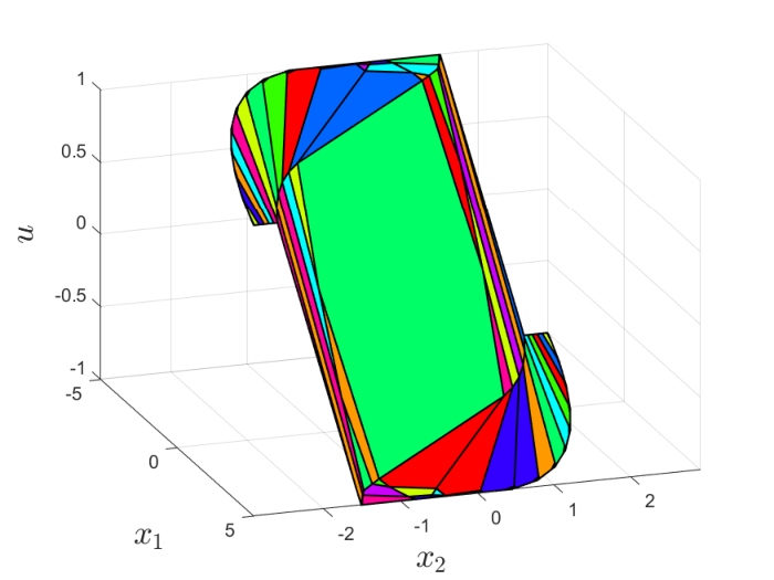
To obtain a neural network approximate of , we sample states uniformly from and compute at these samples as the training data. Through supervised learning with Keras [83], we obtain a ReLU NN controller with hidden layers and neurons in each layer to approximate . The bias term in the output layer of the NN is modified such that . The ReLU NN is visualized in Fig. 4(c). Next, we want to verify the stability of double integrator system under the NN controller .


6.1.2 Estimate ROA through Quadratic/PWQ Lyapunov functions
For the closed-loop system of the double integrator interconnected with , we first apply the ACCPM to search for a quadratic Lyapunov function with . Since the set (Fig. 4(b)) is the ROA of the MPC controller, the ROI is chosen as with a scaling variable to guide our search of Lyapunov functions. Since the estimate of ROA is always contained in the ROI, we want to be as large as possible as long as the ACCPM can find a Lyapunov function.
In the ACCPM implementation, the learner solves the convex program (15) through CVXPY [84] with MOSEK [85] as the solver, and the verifier solves the MIQP (22) through Gurobi [65]. We set in the MIQP (22) and denote the -norm ball centered at the origin with radius . Inside , the closed-loop dynamics is given by
Since has eigenvalues , with norm less than , the closed-loop system is asymptotically stable inside . The ACCPM starts with an empty initial sample set . Through bisection, the largest scaling variable is given by , i.e., we can find a valid quadratic Lyapunov function through the ACCPM with . After iterations, the ACCPM terminated with total solver time seconds and found a valid quadratic Lyapunov function with
| (36) |
together with an estimate of ROA shown in Fig. 6(a). In running the ACCPM, we show the optimal values of the MIQP (22) and the counterexamples found by the verifier in Fig. 5. At termination, the optimal solution of the MIQP (22) is (red star in Fig. 5(b)) which lies on the boundary of with optimal value . This certifies that the terminating parameter in (36) generates a Lyapunov function.
The same procedure is applied to searching PWQ Lyapunov functions with . The ACCPM is initialized with and through bisection on we set . In this case, the ACCPM terminates in iterations with total solver time seconds, and generates a Lyapunov function with
| (37) |
The corresponding estimate of ROA given by the PWQ Lyapunov function is shown in Fig. 6(b). Compared with the quadratic Lyapunov function example in Fig. 6(a), the application of PWQ Lyapunov functions enlarges the estimate ROA found by the ACCPM.
6.1.3 NN controller with projection
We project the synthesized NN controller to the state-dependent polytope shown in (30) with since is a control invariant set under the control input constraint in (35) by construction. By applying the MIQP (34) as the verifier, the ACCPM found a PWQ Lyapunov function with the initial sample set in iterations and with total solver time seconds. Thus, we certify that when the NN controller with projection is applied. As shown in Fig. 7, the corresponding estimate of ROA now becomes a polytope and preserves the asymptotic stability guarantee of the MPC controller constructed in Section 6.1.
6.2 Inverted pendulum with an elastic wall
We use a hybrid system example from [86] and consider the inverted pendulum shown in Fig. 8(a) with parameters . The state is which represents the angle and angular velocity of the pendulum. By linearizing the dynamics of the inverted pendulum around , we obtain a hybrid system which has two modes: not in contact with the elastic wall (mode ) and in contact with the elastic wall (mode ). After discretizing the model using the explicit Euler scheme with a sampling time , a PWA model in the form (5) is obtained with the following parameters
| (38) | ||||
We then synthesize a hybrid MPC controller for the PWA system through disjunctive programming [57] where the control input constraints are given by and the horizon of MPC is set as . The stage and terminal costs are given by
where , and is the solution to the discrete algebraic Riccati equation defined by . We evaluate on a uniform grid samples from the state space and let the reference ROI be the convex hull of all the feasible state samples. Then the ROI with is applied to guide the search for an estimate of ROA.
A total number of feasible samples of state and control input pairs are generated to train a ReLU neural network in Keras to approximate the MPC controller. The NN has hidden layers with neurons in each layer and its output layer bias term is modified after training to guarantee . The NN controller is shown in Fig. 8(b). For the NN controller, we set and verify that the linear closed-loop dynamics inside is asymptotically stable.
With empty initial sample set , the ACCPM is run with both quadratic and PWQ Lyapunov function candidates in order to find a large estimate of ROA. With quadratic Lyapunov function candidates, the largest ROI is given by through bisection on . The ACCPM terminates in iterations with total solver time seconds. The corresponding estimate of ROA is shown in Fig. 9(a). With PWQ Lyapunov function candidates, the largest ROI is given by in which case the ACCPM terminates in iterations with total solver time seconds. The estimate of ROA obtained by the found PWQ Lyapunov function is shown in Fig. 9(b). It is observed that the PWQ Lyapunov function is less conservative compared with the quadratic one. In addition to the theoretical guarantees provided by the ACCPM, the validity of the estimate of ROA is also shown by the simulated closed-loop trajectories in Fig. 9.
7 Conclusion
In this paper, we have proposed an iterative algorithm that learns quadratic and piecewise quadratic Lyapunov functions for piecewise affine systems with ReLU neural network controllers. The proposed algorithm is composed of a learner and a verifier. The learner uses a cutting-plane strategy to propose Lyapunov function candidates from a set of sampled states of the closed-loop system, while the verifier either certifies the validity of the proposed Lyapunov function or rejects it with a counterexample to be accounted for by the learner in the next round. We provide finite-step termination guarantee for the overall algorithm when the set of Lyapunov functions is full-dimensional in the parameter space. Future work includes extending the proposed algorithm to stability analysis of neural-network-controlled uncertain systems.
References
- [1] A. Krizhevsky, I. Sutskever, and G. E. Hinton, “Imagenet classification with deep convolutional neural networks,” in Advances in neural information processing systems, pp. 1097–1105, 2012.
- [2] I. Sutskever, O. Vinyals, and Q. V. Le, “Sequence to sequence learning with neural networks,” in Advances in neural information processing systems, pp. 3104–3112, 2014.
- [3] G. Hinton, L. Deng, D. Yu, G. E. Dahl, A.-r. Mohamed, N. Jaitly, A. Senior, V. Vanhoucke, P. Nguyen, T. N. Sainath, et al., “Deep neural networks for acoustic modeling in speech recognition: The shared views of four research groups,” IEEE Signal processing magazine, vol. 29, no. 6, pp. 82–97, 2012.
- [4] V. Mnih, K. Kavukcuoglu, D. Silver, A. A. Rusu, J. Veness, M. G. Bellemare, A. Graves, M. Riedmiller, A. K. Fidjeland, G. Ostrovski, et al., “Human-level control through deep reinforcement learning,” Nature, vol. 518, no. 7540, pp. 529–533, 2015.
- [5] A. Kurakin, I. Goodfellow, and S. Bengio, “Adversarial examples in the physical world,” arXiv preprint arXiv:1607.02533, 2016.
- [6] N. Papernot, P. McDaniel, S. Jha, M. Fredrikson, Z. B. Celik, and A. Swami, “The limitations of deep learning in adversarial settings,” in 2016 IEEE European symposium on security and privacy (EuroS&P), pp. 372–387, IEEE, 2016.
- [7] A. Abate, D. Ahmed, M. Giacobbe, and A. Peruffo, “Formal synthesis of lyapunov neural networks,” IEEE Control Systems Letters, 2020.
- [8] S. Dutta, S. Jha, S. Sanakaranarayanan, and A. Tiwari, “Output range analysis for deep neural networks,” arXiv preprint arXiv:1709.09130, 2017.
- [9] A. Lomuscio and L. Maganti, “An approach to reachability analysis for feed-forward relu neural networks,” arXiv preprint arXiv:1706.07351, 2017.
- [10] E. Wong and Z. Kolter, “Provable defenses against adversarial examples via the convex outer adversarial polytope,” in International Conference on Machine Learning, pp. 5286–5295, 2018.
- [11] M. Fazlyab, M. Morari, and G. J. Pappas, “Safety verification and robustness analysis of neural networks via quadratic constraints and semidefinite programming,” arXiv preprint arXiv:1903.01287, 2019.
- [12] X. Huang, M. Kwiatkowska, S. Wang, and M. Wu, “Safety verification of deep neural networks,” in International Conference on Computer Aided Verification, pp. 3–29, Springer, 2017.
- [13] A. Raghunathan, J. Steinhardt, and P. S. Liang, “Semidefinite relaxations for certifying robustness to adversarial examples,” in Advances in Neural Information Processing Systems, pp. 10877–10887, 2018.
- [14] G. Katz, C. Barrett, D. L. Dill, K. Julian, and M. J. Kochenderfer, “Reluplex: An efficient smt solver for verifying deep neural networks,” in International Conference on Computer Aided Verification, pp. 97–117, Springer, 2017.
- [15] R. Ehlers, “Formal verification of piece-wise linear feed-forward neural networks,” in International Symposium on Automated Technology for Verification and Analysis, pp. 269–286, Springer, 2017.
- [16] V. Tjeng, K. Xiao, and R. Tedrake, “Evaluating robustness of neural networks with mixed integer programming,” arXiv preprint arXiv:1711.07356, 2017.
- [17] M. Fazlyab, A. Robey, H. Hassani, M. Morari, and G. Pappas, “Efficient and accurate estimation of lipschitz constants for deep neural networks,” in Advances in Neural Information Processing Systems, pp. 11427–11438, 2019.
- [18] M. Fazlyab, M. Morari, and G. J. Pappas, “Probabilistic verification and reachability analysis of neural networks via semidefinite programming,” in 2019 IEEE 58th Conference on Decision and Control (CDC), pp. 2726–2731, IEEE, 2019.
- [19] H. Hu, M. Fazlyab, M. Morari, and G. J. Pappas, “Reach-sdp: Reachability analysis of closed-loop systems with neural network controllers via semidefinite programming,” arXiv preprint arXiv:2004.07876, 2020.
- [20] C. Huang, J. Fan, W. Li, X. Chen, and Q. Zhu, “Reachnn: Reachability analysis of neural-network controlled systems,” ACM Transactions on Embedded Computing Systems (TECS), vol. 18, no. 5s, pp. 1–22, 2019.
- [21] S. Dutta, X. Chen, and S. Sankaranarayanan, “Reachability analysis for neural feedback systems using regressive polynomial rule inference,” in Proceedings of the 22nd ACM International Conference on Hybrid Systems: Computation and Control, pp. 157–168, 2019.
- [22] R. Ivanov, J. Weimer, R. Alur, G. J. Pappas, and I. Lee, “Verisig: verifying safety properties of hybrid systems with neural network controllers,” in Proceedings of the 22nd ACM International Conference on Hybrid Systems: Computation and Control, pp. 169–178, 2019.
- [23] K.-K. K. Kim, E. R. Patrón, and R. D. Braatz, “Standard representation and unified stability analysis for dynamic artificial neural network models,” Neural Networks, vol. 98, pp. 251–262, 2018.
- [24] K. Tanaka, “An approach to stability criteria of neural-network control systems,” IEEE Transactions on Neural Networks, vol. 7, no. 3, pp. 629–642, 1996.
- [25] S. Limanond and J. Si, “Neural network-based control design: an lmi approach,” IEEE Transactions on Neural Networks, vol. 9, no. 6, pp. 1422–1429, 1998.
- [26] H. Yin, P. Seiler, and M. Arcak, “Stability analysis using quadratic constraints for systems with neural network controllers,” arXiv preprint arXiv:2006.07579, 2020.
- [27] M. Jin and J. Lavaei, “Stability-certified reinforcement learning: A control-theoretic perspective,” arXiv preprint arXiv:1810.11505, 2018.
- [28] B. Karg and S. Lucia, “Stability and feasibility of neural network-based controllers via output range analysis,” arXiv preprint arXiv:2004.00521, 2020.
- [29] P. Biswas, P. Grieder, J. Löfberg, and M. Morari, “A survey on stability analysis of discrete-time piecewise affine systems,” IFAC Proceedings Volumes, vol. 38, no. 1, pp. 283–294, 2005.
- [30] G. Ferrari-Trecate, F. A. Cuzzola, D. Mignone, and M. Morari, “Analysis of discrete-time piecewise affine and hybrid systems,” Automatica, vol. 38, no. 12, pp. 2139–2146, 2002.
- [31] M. Johansson and A. Rantzer, “Computation of piecewise quadratic lyapunov functions for hybrid systems,” in 1997 European Control Conference (ECC), pp. 2005–2010, IEEE, 1997.
- [32] M. Rubagotti, L. Zaccarian, and A. Bemporad, “A lyapunov method for stability analysis of piecewise-affine systems over non-invariant domains,” International Journal of Control, vol. 89, no. 5, pp. 950–959, 2016.
- [33] R. Pascanu, G. Montufar, and Y. Bengio, “On the number of response regions of deep feed forward networks with piece-wise linear activations,” arXiv preprint arXiv:1312.6098, 2013.
- [34] M. K.-J. Johansson, Piecewise linear control systems: a computational approach, vol. 284. Springer, 2003.
- [35] S. Prajna and A. Papachristodoulou, “Analysis of switched and hybrid systems-beyond piecewise quadratic methods,” in Proceedings of the 2003 American Control Conference, 2003., vol. 4, pp. 2779–2784, IEEE, 2003.
- [36] S. Boyd, L. El Ghaoui, E. Feron, and V. Balakrishnan, Linear matrix inequalities in system and control theory. SIAM, 1994.
- [37] U. Topcu, A. Packard, P. Seiler, and T. Wheeler, “Stability region analysis using simulations and sum-of-squares programming,” in 2007 American Control Conference, pp. 6009–6014, IEEE, 2007.
- [38] N. M. Boffi, S. Tu, N. Matni, J.-J. E. Slotine, and V. Sindhwani, “Learning stability certificates from data,” arXiv preprint arXiv:2008.05952, 2020.
- [39] J. Kapinski, J. V. Deshmukh, S. Sankaranarayanan, and N. Arechiga, “Simulation-guided lyapunov analysis for hybrid dynamical systems,” in Proceedings of the 17th international conference on Hybrid systems: computation and control, pp. 133–142, 2014.
- [40] A. Solar-Lezama, L. Tancau, R. Bodik, S. Seshia, and V. Saraswat, “Combinatorial sketching for finite programs,” in Proceedings of the 12th international conference on Architectural support for programming languages and operating systems, pp. 404–415, 2006.
- [41] A. Solar-Lezama and R. Bodik, Program synthesis by sketching. Citeseer, 2008.
- [42] D. Ahmed, A. Peruffo, and A. Abate, “Automated and sound synthesis of lyapunov functions with smt solvers,” in International Conference on Tools and Algorithms for the Construction and Analysis of Systems, pp. 97–114, Springer, 2020.
- [43] H. Ravanbakhsh and S. Sankaranarayanan, “Learning control lyapunov functions from counterexamples and demonstrations,” Autonomous Robots, vol. 43, no. 2, pp. 275–307, 2019.
- [44] I. E. S. Tarasov, L. G. Khachiyan, “The method of inscribed ellipsoids,” Soviet Mathematics Doklady, vol. 37, 1988.
- [45] W. M. Haddad and V. Chellaboina, Nonlinear dynamical systems and control: a Lyapunov-based approach. Princeton university press, 2011.
- [46] E. Polak, Optimization: algorithms and consistent approximations, vol. 124. Springer Science & Business Media, 2012.
- [47] D. S. Atkinson and P. M. Vaidya, “A cutting plane algorithm for convex programming that uses analytic centers,” Mathematical Programming, vol. 69, no. 1-3, pp. 1–43, 1995.
- [48] J. Elzinga and T. G. Moore, “A central cutting plane algorithm for the convex programming problem,” Mathematical Programming, vol. 8, no. 1, pp. 134–145, 1975.
- [49] S. Boyd and L. Vandenberghe, “Localization and cutting-plane methods,” From Stanford EE 364b lecture notes, 2007.
- [50] A. Y. Levin, “An algorithm for minimizing convex functions,” Soviet Mathematics Doklady, vol. 160, pp. 1244–1247, 1965.
- [51] L. G. Khachiyan, “Polynomial algorithms in linear programming,” USSR Computational Mathematics and Mathematical Physics, vol. 20, no. 1, pp. 53–72, 1980.
- [52] D. Y. A.S. Nemirovskii, “Problem complexity and method efficiency in optimization,” 1983.
- [53] P. M. Vaidya, “A new algorithm for minimizing convex functions over convex sets,” in 30th Annual Symposium on Foundations of Computer Science, pp. 338–343, IEEE, 1989.
- [54] J.-L. Goffin and J.-P. Vial, “On the computation of weighted analytic centers and dual ellipsoids with the projective algorithm,” Mathematical Programming, vol. 60, no. 1-3, pp. 81–92, 1993.
- [55] Y. Nesterov, “Cutting plane algorithms from analytic centers: efficiency estimates,” Mathematical Programming, vol. 69, no. 1, pp. 149–176, 1995.
- [56] S. Boyd, S. P. Boyd, and L. Vandenberghe, Convex optimization. Cambridge university press, 2004.
- [57] T. Marcucci and R. Tedrake, “Mixed-integer formulations for optimal control of piecewise-affine systems,” in Proceedings of the 22nd ACM International Conference on Hybrid Systems: Computation and Control, pp. 230–239, 2019.
- [58] F. Borrelli, A. Bemporad, and M. Morari, Predictive control for linear and hybrid systems. Cambridge University Press, 2017.
- [59] T.-W. Weng, H. Zhang, H. Chen, Z. Song, C.-J. Hsieh, D. Boning, I. S. Dhillon, and L. Daniel, “Towards fast computation of certified robustness for relu networks,” arXiv preprint arXiv:1804.09699, 2018.
- [60] H. Zhang, T.-W. Weng, P.-Y. Chen, C.-J. Hsieh, and L. Daniel, “Efficient neural network robustness certification with general activation functions,” in Advances in neural information processing systems, pp. 4939–4948, 2018.
- [61] M. Hein and M. Andriushchenko, “Formal guarantees on the robustness of a classifier against adversarial manipulation,” in Advances in Neural Information Processing Systems, pp. 2266–2276, 2017.
- [62] S. Wang, K. Pei, J. Whitehouse, J. Yang, and S. Jana, “Efficient formal safety analysis of neural networks,” in Advances in Neural Information Processing Systems, pp. 6367–6377, 2018.
- [63] L. A. Wolsey and G. L. Nemhauser, Integer and combinatorial optimization, vol. 55. John Wiley & Sons, 1999.
- [64] C.-T. Chen, Linear System Theory and Design. USA: Oxford University Press, Inc., 2nd ed., 1995.
- [65] L. Gurobi Optimization, “Gurobi optimizer reference manual,” 2020.
- [66] P. Belotti, C. Kirches, S. Leyffer, J. Linderoth, J. Luedtke, and A. Mahajan, “Mixed-integer nonlinear optimization,” Acta Numerica, vol. 22, p. 1, 2013.
- [67] S. Vigerske, “Decomposition in multistage stochastic programming and a constraint integer programming approach to mixed-integer nonlinear programming,” 2013.
- [68] M. Tawarmalani and N. V. Sahinidis, Convexification and global optimization in continuous and mixed-integer nonlinear programming: theory, algorithms, software, and applications, vol. 65. Springer Science & Business Media, 2013.
- [69] P. Belotti, J. Lee, L. Liberti, F. Margot, and A. Wächter, “Branching and bounds tighteningtechniques for non-convex minlp,” Optimization Methods & Software, vol. 24, no. 4-5, pp. 597–634, 2009.
- [70] R. E. Moore, R. B. Kearfott, and M. J. Cloud, Introduction to interval analysis. SIAM, 2009.
- [71] Y. Ye, “A potential reduction algorithm allowing column generation,” SIAM Journal on Optimization, vol. 2, no. 1, pp. 7–20, 1992.
- [72] Z.-Q. Luo and J. Sun, “A polynomial cutting surfaces algorithm for the convex feasibility problem defined by self-concordant inequalities,” Computational Optimization and Applications, vol. 15, no. 2, pp. 167–191, 2000.
- [73] J.-L. Goffin, Z.-Q. Luo, and Y. Ye, “Complexity analysis of an interior cutting plane method for convex feasibility problems,” SIAM Journal on Optimization, vol. 6, no. 3, pp. 638–652, 1996.
- [74] J. Sun, K.-C. Toh, and G. Zhao, “An analytic center cutting plane method for semidefinite feasibility problems,” Mathematics of Operations Research, vol. 27, no. 2, pp. 332–346, 2002.
- [75] A. A. Ahmadi and P. A. Parrilo, “Non-monotonic lyapunov functions for stability of discrete time nonlinear and switched systems,” in 2008 47th IEEE Conference on Decision and Control, pp. 614–621, IEEE, 2008.
- [76] D. Aeyels and J. Peuteman, “A new asymptotic stability criterion for nonlinear time-variant differential equations,” IEEE Transactions on automatic control, vol. 43, no. 7, pp. 968–971, 1998.
- [77] R. Bobiti and M. Lazar, “A sampling approach to finding lyapunov functions for nonlinear discrete-time systems,” in 2016 European Control Conference (ECC), pp. 561–566, IEEE, 2016.
- [78] S. Chen, K. Saulnier, N. Atanasov, D. D. Lee, V. Kumar, G. J. Pappas, and M. Morari, “Approximating explicit model predictive control using constrained neural networks,” in 2018 Annual American control conference (ACC), pp. 1520–1527, IEEE, 2018.
- [79] D. Simon and J. Löfberg, “Stability analysis of model predictive controllers using mixed integer linear programming,” in 2016 IEEE 55th Conference on Decision and Control (CDC), pp. 7270–7275, IEEE, 2016.
- [80] B. Karg and S. Lucia, “Efficient representation and approximation of model predictive control laws via deep learning,” IEEE Transactions on Cybernetics, 2020.
- [81] A. Bemporad, M. Morari, V. Dua, and E. N. Pistikopoulos, “The explicit linear quadratic regulator for constrained systems,” Automatica, vol. 38, no. 1, pp. 3–20, 2002.
- [82] M. Herceg, M. Kvasnica, C. Jones, and M. Morari, “Multi-Parametric Toolbox 3.0,” in Proc. of the European Control Conference, (Zürich, Switzerland), pp. 502–510, July 17–19 2013. http://control.ee.ethz.ch/˜mpt.
- [83] F. Chollet et al., “Keras,” 2015.
- [84] S. Diamond and S. Boyd, “CVXPY: A Python-embedded modeling language for convex optimization,” Journal of Machine Learning Research, vol. 17, no. 83, pp. 1–5, 2016.
- [85] M. ApS, The MOSEK optimization toolbox for Python manual. Version 9.2, 2020.
- [86] T. Marcucci, R. Deits, M. Gabiccini, A. Bicchi, and R. Tedrake, “Approximate hybrid model predictive control for multi-contact push recovery in complex environments,” in 2017 IEEE-RAS 17th International Conference on Humanoid Robotics (Humanoids), pp. 31–38, IEEE, 2017.