Ejection-collision orbits in two degrees of freedom problems in celestial mechanics
Abstract.
In a general setting of a Hamiltonian system with two degrees of freedom and assuming some properties for the undergoing potential, we study the dynamics close and tending to a singularity of the system which in models of -body problems corresponds to total collision. We restrict to potentials that exhibit two more singularities that can be regarded as two kind of partial collisions when not all the bodies are involved. Regularizing the singularities, the total collision transforms into a 2-dimensional invariant manifold. The goal of this paper is to prove the existence of different types of ejection-collision orbits, that is, orbits that start and end at total collision. Such orbits are regarded as heteroclinic connections between two equilibrium points and are mainly characterized by the partial collisions that the trajectories find on their way. The proof of their existence is based on the transversality of 2D-invariant manifolds and on the behavior of the dynamics on the total collision manifold, both of them are thoroughly described.
1. Introduction
In Celestial Mechanics the goal is to understand the dynamical behavior of particles which interact under their mutual newtonian gravitational attraction. Although many studies have been devoted to this problem, whose dynamics turns out to be tremendously rich from a dynamical point of view, it is very far from being well understood. A particular critical point to understand the dynamics of the -body problem is to identify the behavior near the total collision and the escape to infinity. This is typically done by introducing a boundary total collision manifold for each of the energy surfaces and by constructing the missing components of its boundary as other submanifolds, which represent the asymptotic behavior at infinity. This can be obtained, first, through a McGehee’s change of coordinates (plus a scaling of time) that allows to blow up the origin (where the total collision of the bodies takes place), and, secondly, by generalizing McGehee’s change of variable in the configuration space to blow up the infinity. See [15], [6], and [18] on how to apply the blow up of the origin for different three or four body problems. In [8] surges this novel idea of blowing up the infinity, where the authors study the total collision and infinity manifolds associated to several problems.
An intriguing question is concerned with the so called ejection-collision orbits (ECO), that is, trajectories where all the bodies eject from the same point and after some time they collide at the same point. Taking into account the collision manifold, ECO may be regarded as heteroclinic connections between suitable hyperbolic equilibrium points of the blown up dynamical system, that is, ECO are obtained from the intersection of the invariant manifolds associated with these equilibrium points. Simó and Llibre 1981 consider the -body problem in (being any dimension), and characterize the transversality between these stable and unstable manifolds. A general reference for collisions in -body problems is due to Saari 2005.
In this paper, we consider the general system of ODE with two degrees of freedom:
| (1) |
where , , is a diagonal constant matrix, , , , and is an homogeneous function of degree -1 on . We remark that such a system defines a general setting that, in particular, includes some subproblems of the -body problem. Moreover is singular in , that corresponds to all the possible collisions between the bodies (in the context of the -body problem). In particular corresponds to the total collision of all the bodies. A main goal of this paper is focussed on the ejection-collision orbits. More concretely, we want to prove the existence of ECO under certain conditions of the potential (that will appear later on). We will follow the ideas already used, for specific problems, by McGehee, Lacomba, Saari, Kaplan, etc. One direction to tackle this problem has been to consider few body problems, as the collinear three body problem [15, 7] or the isosceles three body problem [6]. Some others have some symmetries involved, as the symmetric collinear four body problem [10, 1, 4], the trapezoidal four body problem [9, 3, 2], and the rhomboidal four body problem [5] and [12]. Some of them depend on parameters associated to the masses.
These problems have been given much attention, and they share several common properties that we generalize and use to obtain information to prove analytically the existence of ECOs. In a prior paper by the authors of this article [4], a family of ECO was obtained from a numerical point of view in the symmetric collinear four body problem.
Our main objectives are two. First, in a general setting of a Hamiltonian system of two degrees of freedom as in Eq. (1) with a potential with specific characteristics, to describe the main characteristics of its dynamics in which the collision manifold play a key role. This is done in Sections 2 and 3. Secondly, to prove the existence and to give a classification of the ECO that can be obtained depending on the specific behavior of the 1D-invariant manifolds on the total collision manifold. The main results are given in Theorems 1–4. In order to accomplish our aims, we will review and show results already known in specific three and four body problems, where we shall see that the dynamics are essentially the same. So, we will recover here all of them.
2. General setting
In this section, we give the conditions for the undergoing potential, in (1), recall some particular examples, derive the regularized equations of the model and present the main features (we consider a suitable Poincaré section and define the collision manifold) that will play an essential role along the paper.
2.1. Statement of the problem
We consider the problem defined by a Hamiltonian system with two degrees of freedom and Hamiltonian function
| (2) |
, , is a diagonal constant matrix, , , , and is an homogeneous function of degree with some properties to be specified later. We can think of an -body problem with the Newtonian potential (we will show some of these problems later), where is a singularity that corresponds to the total collision of the bodies. The model was also considered, for example, by Martínez 2012, Martínez 2013 to study the existence of Shubart-like orbits. Here, we recall some known features of the model. For more details see the aforementioned articles.
It is well known that the Hamiltonian is a constant of motion for the -body problem. We confine our attention to a fixed negative level of energy . Thus, we have the following classical result.
Proposition 1.
Consider the Hamiltonian system given by (2). Then, bounded motion can only occur for .
The proof of this result is based on the Lagrange-Jacobi equation , where is the moment of inertia, and the fact that is a homogeneous function of degree . See, for instance, Proposition 4.1 in [16].
Our goal is to study the existence of ejection-collision orbits (ECO from now on). Roughly speaking, an ejection orbit is an orbit that “starts” at , and a collision orbit is an orbit that “ends” at (we give the precise definition later on). Therefore, it is mandatory to regularize the singularity . Regularization theory is a tool that allows us to transform a singular differential equation into a regular one, in such a way that we can analyze, under the regularized equations, the behavior of solutions leading to collisions.
We use McGehee’s coordinates [15], that not only regularize but perform a blow up of the total collision . First, the following change to a polar-like set of coordinates , , is introduced:
where . Differentiating, can be written as
where , so that , , and the radial component of the velocity is given by . Next, variables , are defined as
so that .
Introducing the new coordinates together with the scaling in time given by , the equations of motion become
| (3) |
where and . Clearly, the system of equations (3) can be extended to , which is an invariant manifold of the system.
The energy relation in these new variables is written as
| (4) |
Notice that for any fixed energy level ,
| (5) |
is the zero velocity curve which limits the region in configuration space where the motion is admissible (see Figure 1).
We want to prove the existence of ECO under certain conditions for the potential . As it is common in this kind of problems, the leading actors in the dynamics of the problem are the invariant manifold , the existence of unstable equilibrium points and the behavior of the invariant manifolds associated to them. Next result states the hypotheses on the potential to ensure the existence of the key ingredients.
Proposition 2.
Assume that is such that
where for fixed values , such that , and
- •
, are constants, and if and only if ;
- •
is a smooth bounded function in ;
- •
has only one non-degenerate critical value at , which is a minimum.
Then, the system of equations (3) has two equilibrium points, denoted by , given by , , , , where . Both equilibrium points are saddle points, and there exist invariant manifolds . Restricted to a fixed energy level , , and , .
See [13] for the proof of the last proposition, and a discussion about the linear approximation of the invariant manifolds depending on . Simó and Llibre [19] give a condition on the potential at the critical point to prove the existence of transversal intersection of the invariant manifolds associated to total collision and total ejection in a general -body problem of dimension . In our case, the condition is fulfilled by the fact that is a non-degenerate critical value.
In Figure 1 we show the configuration space , which is a subset of the half-cone limited by the zero velocity curve (5).
In the models of -body problems, when a collision between two or more bodies occurs, the distance between them becomes zero and the velocity of the colliding particles is infinite. This corresponds to a singularity for Newton’s equations. As we mentioned, one kind of collision occurs when all particles of the system collide simultaneously, and corresponds to . In fact, the manifold defined as
| (6) |
is invariant under the flow given by equations (3), and it is called the total collision manifold. By Proposition 2, the equilibrium points .
It is relevant that the flow on is almost-gradient with respect to , see [15]. That is, introducing the energy relation (4) in the second equation of system (3), , so when , . Later on, we will strongly use this property of the flow on the total collision manifold .
Other singularities appear when “partial” collisions occur, that is, collisions when not all of the bodies are involved. The simplest one, a binary collision, arises when two bodies occupy the same point. Also there can be collisions of more than two bodies or simultaneous collisions of different clusters of particles. Under the hypotheses of Proposition 2, these additional singularities occur at . Therefore, we will say that we have a collision of type or depending on whether or .
Next we define ejection and collision orbits. These are orbits that tend, backwards and forwards respectively, to , so they belong to the invariant manifolds of the equilibrium points . As we will see, the one dimensional invariant manifolds are embedded in the collision manifold , so we only consider the trajectories on the two dimensional invariant manifolds for their definition.
Definition 1.
We say that an orbit is a collision orbit if it is contained in and an ejection orbit if it is contained in An orbit is an ejection–collision orbit if it is contained in
Therefore, an ejection-collision orbit (ECO) satisfies
From now on, we consider that we are under the hypotheses of Proposition 2 and the energy is fixed at a value .
2.2. Examples from Celestial Mechanics
Next, we provide a few examples of problems from Celestial Mechanics that match the general model presented.
- •
The rectangular four body problem (Rec4BP). In this problem, four equal masses lie at the vertices of a rectangle, so that their positions and velocities are symmetric with respect to two axes, vertical and horizontal, passing through their center of mass, placed at the origin. Its potential can be written as
for . The two singularities correspond to two double collisions. See, for example, [18, 11].
- •
The rhomboidal four body problem (Rh4BP). In this problem, there are two different pairs of equal mass particles, and and is the mass ratio between them. The bodies are placed at the vertices of a rhombus with initial positions and velocities symmetric with respect to the diagonals of the rhombus. The potential is given by
for . As in the previous example, the two singularities correspond to two double collisions. See, for example, [5, 12].
- •
The symmetric collinear four body problem (SC4BP). In this problem four bodies of masses, , , , and , , are collinear, ordered from left to right and moving symmetrically by pairs about their center of mass. In this case, the potential writes
for , where . The singularity corresponds to double binary collisions between and , and and , and the singularity corresponds to single binary collisions between and . See, for example, [10, 3, 4].
- •
The collinear three body problem (C3BP), where three masses and form a collinear configuration, labelled from left to right. The potential is given by
where and is a constant depending on the masses of the system. The singularities correspond to collisions of the left binaries, , or collisions of the right binaries, . See [15, 7].
- •
A symmetric planar body problem. Consider equal masses located in a configuration in which the mass is symmetric to with respect the line , . Due to the symmetries of the problem, it reduces to a two degrees of freedom system with potential
for , and analytic. See, for example, [14].
2.3. Regularization of non-total collisions
In the present model, the system of equations (3) has singularities at and . These singularities correspond to distinct partial collisions for the different -body problems. For instance, for the Rec4BP, both singularities correspond to double binary collisions between two different pairs of bodies, whereas for the SC4BP, corresponds to a double binary collision of the two particles on the left and the two particles on the right, and corresponds to a single binary collision of the two particles at the center.
The two singularities at can be removed simultaneously through a Sundman type regularization. See [13], and the references therein for more details. Consider the functions
where if , and otherwise. Notice that is a positive and bounded smooth function in . Then, introducing a new variable and the change of time
the system of equations (3) transforms into
| (7) |
where .
The energy relation (4), in these new variables, writes
| (8) |
Notice that if is a solution with energy , then is also a solution with energy , with . Therefore, it is enough to fix any negative value for .
We will study the system of differential equations (7) in the regularized and reduced McGehee coordinates on the phase space , . A solution of the above set of ordinary differential equations, also called orbit, will be denoted by (or just by ), where .
Notice that system (7) exhibits the symmetry
| (9) |
This can be phrased in terms of solutions as follows: if is a solution then defined as:
| (10) |
is also a solution.
The claim of Proposition 2 persists in the new variables, so system (7) has two hyperbolic equilibrium points , with coordinates . Next result states the existence of an orbit that connects both equilibrium points (see [13]). It is called the homothetic solution because the configuration maintains the same shape along its evolution for all the time, only changing its size.
Proposition 3.
For every fixed level of energy , there exists a solution of the system of equations (7) of the form
such that .
Notice that this is an ejection-collision orbit since it starts and ends at .
2.4. Poincaré section and map
In this section we introduce a convenient Poincaré section, which shall be a keystone to show the existence of ECO. We consider as a Poincaré section the set where partial collisions occur, that is, where . Notice that, from the energy relation (8), any point on also must satisfy .
Definition 2.
We denote by is the union of two half planes :
Next, we present a property which shows that if a solution is such that the variable is on the right side of increasingly, or on the left side but decreasingly, then the orbit must reach the section . It has been proved useful in the context of different -body problems, as shown in [7, 20] for the C3BP or [17, 10, 4] for the SC4BP.
Proposition 4.
Let be a solution of the system given by (7) such that a certain time , either and or and . Then, the trajectory must reach the section at least once.
Proof.
We may assume that and , and we will see that the orbit must reach the section . In the other scenario, the orbit must reach , and it can be proved using the same arguments.
First, let us prove that cannot reach a maximum at and . Indeed, assume there exists such that, , and for . From the properties of function , we have that , , and using equations (7) and (8) we obtain
so has a minimum in , but this is impossible since increases in .
Since is bounded between and , then either
- (i)
reaches and the proposition is proved;
- (ii)
or tends asymptotically to . Let us prove that this situation is not possible. The corresponding solution would satisfy that
However, using equation (7), if and , then , which is a contradiction.
∎
In Figure 1 right, we show an orbit of the SC4BP exhibiting different partial collisions (when ) and crossings with the section . Actually, in [17], the authors use this later section to construct a Poincaré map in order to describe the dynamics for this problem. However, in general, a trajectory experiences a sequence (maybe finite) of partial collisions, where the solution reaches . This idea has been exploited by different authors when studied the three and four body problems mentioned in Section 2.2, by introducing symbolic dynamics and characterizing the orbits by the sequence of partial collisions that they suffer. See, for example, [7, 20, 10, 17, 4], and references therein. In [7, 10, 4] the authors show that, in order to deal with ejection-collision orbits, the use of is quite more appropriate.
We will follow the same idea. We consider the Poincaré map (in forward time) defined on
| (11) |
as , where is the flow associated to the system (7), and is the first positive time needed to reach the section starting at . In a similar way we define , the Poincaré map in backward time.
2.5. Collision manifold
We have already defined the total collision manifold in (6), and for simplicity, in the new variables the total collision manifold is also denoted by . It corresponds to equation (8) for and it is a 2-dimensional manifold, topologically equivalent to a sphere minus four points, independent of the total energy , see Figure 2. It is invariant under the flow (7), which is gradient-like with respect the variable , that is, . It is also the boundary of the energy constant manifold , for every fixed level of energy . We can think the space as a book of infinite sheets where a fixed level of energy corresponds to a sheet of the book, and the spine corresponds to the zero level of energy, which is precisely the total collision manifold.

Next results provide us with useful information about the solutions on the total collision manifold , information that later will be meaningful to describe the dynamics of the invariant manifolds of .
Lemma 1.
Consider the system given by (7) on the manifold and a solution . Then, all the maxima and minima of correspond to points where and either or .
Proof.
Proposition 5.
On the collision manifold , any solution is such that the variable oscillates from maxima to minima on and/or the curve , .
Proof.
In Figure 3 we show some orbits on the collision manifold in the SC4BP for different values of the parameter of the problem.
Remark. As a consequence of Proposition 4, any solution in is such that forwards in time, either oscillates infinitely between maxima and minima while , or oscillates a finite number until the orbit tends to (analogously backwards in time). In particular any heteroclinic orbit connecting and will describe a finite number of oscillations between and .
Notice that on the collision manifold the variables and are bounded, whereas the variable . When a solution of equations (7) on is such that , we say that it escapes through the right arm if , respectively through the left arm if .
3. Dynamics on the invariant manifolds
As stated in previous sections, on one hand, the problem given by equations (7) has a collision manifold corresponding to the blow-up performed at , and on the other hand, there exist two hyperbolic equilibrium points, , and their corresponding invariant manifolds, see Proposition 2. The knowledge of the qualitative behavior of the flow on the total collision manifold will lead us to read off the behavior of orbits passing near total collision, ejecting from or reaching total collision.
As stated in Proposition 2, the equilibrium points are hyperbolic and, for a fixed value of the energy , each one has associated two invariant manifolds: one of dimension one, the other of dimension two. Due to the symmetry (9), the invariant manifolds associated to are symmetric to the ones associated to . Therefore, it is enough to describe the behavior of, for example, . These invariant manifolds are already well known and studied in the three and four body problems mentioned in Section 2.2, see for example, [6, 9, 18]. In the next section we will describe their behavior in detail and establish some nomenclature.
3.1. One dimensional invariant manifolds
We start by describing the behavior of (and by symmetry, we have that of ), which is a one dimensional invariant manifold with two branches, each one being specific solutions of the system. We will denote by (respectively ) the branch going torwards the half-space (resp. ). Notice that also, by the third equation of (7), the positive branch goes towards , whereas the negative branch moves towards . The first important property is that . Second, as we have seen in Section 2.5, any given branch is an orbit that initially goes back and forth between and and then it can only exhibit two different behaviors: either it tends to (becoming an heteroclinic connection) or the trajectory “escapes” towards along one of the upper legs of the total collision manifold. See Figures 3 and 4.
There exist three possible cases, named after Lacomba [9]. The non-degenerate case, in which there are no heteroclinic connections on between the equilibrium points and the branches of go through the upper legs of (Figure 3). In the symmetric degenerate case, both branches of coincide with the branches of , so there exist two heteroclinic connections between the equilibrium points (Figure 4, center). In the (non-symmetric) degenerate case, only one branch of coincides with one branch of , while the other branch of escapes along one of upper legs of (Figure 4, left and right).
Observe that in the non-degenerate case, initially both branches of the invariant manifolds go through partial collisions alternatively, and then exhibit the same type of partial collisions going up along one upper arm of . In the degenerate cases, the branches corresponding to heteroclinic connections only exhibit a finite number of partial collisions.
In fact, the branches of the one dimensional invariant manifolds can be characterized by the number of full turns around the total collision manifold (the number of oscillations of the variable between and ). More concretely, we say that a branch of a 1D-invariant manifold makes a full turn if the variable varies from to passing through and just once. For example, the orbits on Figure 3 top left, make two full turns, whereas those on plot top right make one and a half turn.
The number of full turns and their intersections with the section allow us to characterize the 1D-invariant manifolds as follows. Consider the successive intersections of each branch with the the section (see Definition 2)
where , and , are increasing sequences (see Figure 3). In the non-degenerate cases the sequences are infinite, whereas in the degenerate cases some or all of them are finite. Notice that, using the symmetry of the system we have that
For simplicity, we will simply just denote by the points , , respectively.
Let be the set of all possible sequences, just taking into account the elements and . We define
where
The sequence codes the partial collisions (intersections with ) forwards in time for the unstable manifold. Similarly, we can define on , obtaining a sequence of partial collisions backwards in time. Using the symmetry of the problem we have that
We classify the behavior of the 1-dimensional manifolds and using the number of full turns of each branch, their intersections with the section and the map . In what follows, the sequence denotes that the sequence is repeated times. For example, the sequence represents an orbit with a sequence of pairs of collisions (a collision of type followed by a collision of type ) and then the orbit only has collisions of type forwards in time. Analogous interpretations are given for other sequences.
The non-degenerate cases are classified in four types:
- (1)
Type I: Both branches make full turns around (see Figure 3 top left), before escaping through different arm:
Then, the sequences and are ordered as follows. Along the line :
Along the line :
see Figure 5.


Figure 5. Ordering of sequences (see Section 3.1) and (see Section 3.2) along for the non-degenerate case Type I. Figures left and right represent bottom and top parts of , respectively. - (2)
Type II: Both branches make full turns and a half (see Figure 3 top right), before escaping through a different arm on :
Then, the sequences and on are ordered as follows:
To obtain the ordering on , change the sign plus by minus.
- (3)
Type III: The positive branch makes full turns whereas the negative branch makes and a half (see Figure 3 bottom left), before escaping both through the right arm:
The sequences and along satisfy
In this case, along we have the following ordered finite sequence:
- (4)
Type IV: The positive branch makes full turns and a half whereas the negative branch makes turns (see Figure 3 bottom right), before escaping both through the left arm:
In this case, along there is a finite number of intersections:
Along the ordering is the following:
Along the paper, we will refer to each one of the above cases. We summarize them in Table 1.
| Type | ||
|---|---|---|
| I | ||
| II | ||
| III | ||
| IV |
In the degenerate cases, there are three cases. If it is non-symmetric, one of the branches connect with the equilibrium point , so its image by is a finite sequence, whereas the other one exhibits one of the behaviors described above. In the symmetric degenerate case, both branches have associated a finite sequence in , see Figure 4.
3.2. Two dimensional invariant manifolds
Next, we describe some features of the behavior of the 2-dimensional invariant manifolds and . In Figure 6 we show a qualitative representation of such invariant manifolds. We observe that if , then the projection of the motion in the space takes place inside the collision manifold. This can be deduced from equation (8). For fixed, the motion takes place in an ellipse in the plane with semiaxes that are maxima when (since ): and
However we plot the manifolds outside for a clearer visualization (following the first plots by Lacomba et al.)
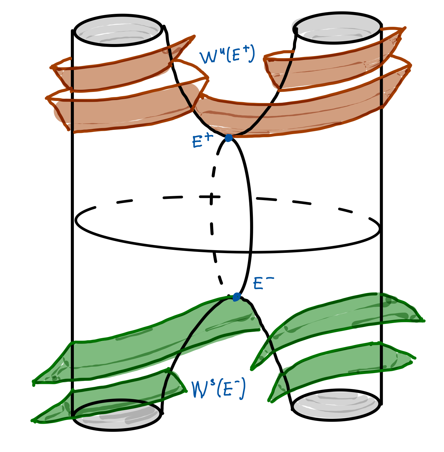
More concretely:
- •
The invariant manifolds are glued to the total collision manifold , not only by the equilibrium point: the intersections are
(12) where each (resp. ) is an orbit that escapes forwards (respectively backwards) in the -direction, (resp. ) through one of the legs of (see, for instance [7] or [8]). Here, as for the one dimensional invariant manifolds, the sign (respectively the sign ) means that the orbit initially moves with space (respespectively ) near the equilibrium point, when referring to and for . See Figure 7.
As explained in Section 2.5, each trajectory performs an infinite sequence of partial collisions:
and
In fact,
where , , and
with , . The sequences are increasing and are decreasing (). See Figure 7.
These sequences can be combined with the sequences and . In all the cases it is clear that
(13) See for example Figure 5 for the non-degenerate case of Type I.
- •
The solution given in Proposition 3 belongs to , that is, it is an ECO that connects both equilibrium points without any partial collision. Therefore, does not intersect .

From now on, we will simply just denote by the points , , respectively.
4. Ejection-Collision Orbits
In this section we prove the existence of the different types of ECO depending on the behavior of the 1-dimensional invariant manifolds. Actually, we will characterize the ECO by its finite number of successive binary collisions with . Let be a finite sequence of collisions of type and . Following the notation in Section 3.1, we will say that an ECO is of type if its orbit describes forwards in time the finite sequence of binary collisions encoded by .
The following result is straightforward from the symmetry (9).
Proposition 6.
Let be an ECO of type . Then defined as in (10) is an ECO of type , with , .
Along the proofs of the following results, we use the notation and for the interior and the closure of a set .
We start with a technical lemma and a general result for all the cases. We will denote by and the first intersection (forwards and backwards in time, respectively) of the 2-dimensional manifolds with each one of the sections .
Lemma 2.
Each one of the intersections and is an arc contained in whose closure has endpoints contained on . More precisely,
| (14) |
where denotes a closed arc contained in with endpoints .
Proof.
We detail the proof for . The intersection with follows similar arguments, and the intersections of the stable manifold of are obtained using the symmetry of the problem. Let be the flow of system (7).
Consider an arc of initial conditions contained in and close enough to , so that the arc is homeomorphic to a semicircle parametrized by an angle , in such a way that correspond to points in and in respectively (recall (12)), and corresponds to a point in the homothetic orbit . See Figure 8.
Clearly, intersects at . Therefore, by continuity, the flow transforms the subarc parameterized by into a continuous arc contained in . Moreover, for any in this subarc close to , the trajectory has a close passage to . Due to the hyperbolic character of the equilibrium point, the orbit will continue close to the unstable branch of , whose intersection with is . Therefore, is an arc with end points and .
In a similar way, the image of the subarc parametrized by is also a continuous arc, contained in , with endpoints and . ∎
In Figure 8, we show the idea of the proof of the Lemma 2. The projection of the collision manifold in the plane and the semiplane , (that contain the projection of the arches) are depicted jointly glued to the section . From now on, the pictures will follow this representation.

Theorem 1.
For any natural number , the system (7) has an ejection-collision orbit of type
Proof.
From Lemma 2, recall that and are the four arcs that correspond to the first intersection of the unstable and stable manifolds, respectively, with . We give a proof of the existence of ECOs with only collisions of type . The result for the other type of ECOs follows by repeating the same arguments considering the other branches of the invariant manifolds and section .
For , from Lemma 2 and the ordering (13), it follows that . Let us denote by the point such that the arc does not intersect except at . Clearly for with no other partial collisions. Thus, it is an ECO of type , see Figure 8.

To prove the claim for any , we will follow the stable manifold backwards in time to look for intersections with . Recall that is the Poincaré map (see (11)). Notice that and are defined for any point on that does not correspond to an ECO.
We claim that is an arc contained in whose closure is the arc , that is, . On the one hand, it is clear that . Consider close to , and its orbit . Applying the same argument as in Lemma 2, the trajectory in backwards time will have a close passage to the equilibrium point and then will follow the branch . Therefore,
Using the ordering of the points along (see Section 3.1 and Figure 5), intersects at a point that corresponds to an ECO of type .
Now consider such that the arc does not intersect except at . Using the same argument as before, , which intersects . Therefore, there exists an ECO of type .
By induction, and there exists such that the arc does not intersect except at point . Therefore, for each , there exists a point on that corresponds to an ECO of type , with partial collisions of type b. ∎
We notice that the results and proofs of Lemma 2 and Theorem 1 follow the same arguments as in the case of the C3BP ([7]) or in the SC4BP ([10]). We remark that we are analyzing a more general setting.
4.1. Non-degenerate cases
Next, we will prove the existence of ECO exhibiting different number and type of partial collisions. The results will depend on the behavior of the 1D-invariant manifolds contained in the collision manifold , classified in types I, II, III and IV in Section 3.1, and the orderings explained in that section.
Theorem 2.
Suppose that are of type I, and let be the number of full turns performed by the branches of the 1D-invariant manifolds before escaping through different arms of . Then:
- (a)
There exist ejection-collision orbits exhibiting collisions of types
and
- (b)
There exist ejection-collision orbits exhibiting any sequence that can be obtained by the following graph:
Proof.
Recall that the fact that are of type I means that the branches perform full turns and exhibit the following behaviors respectively (see Table 1 and Figure 3, top left):
Therefore, as shown in Section 3.1, the intersections of the 1D-invariant manifolds with the section give the sequences , with a specific ordering, see also Figure 5.
From Lemma 2, and are the arcs that correspond to the first intersection, backwards and forwards in time, of and with , respectively (similarly, and and the section ). In Theorem 1, we have proved that ().
The arguments are done by iterating the Poincaré map backwards in time and following the preimages of the stable manifold to look for intersections with .
Remark. In most of the figures that illustrate the proofs, for simplicity, those arcs that intersect are shown as if they would intersect only once. In general, this is not necessarily the case. For this reason, in the proofs the reader will find points like and that in the figures seem to be the same one, but they are not in general.
- (a)
First, we shall prove the existence of ECO of the form . The existence of an ECO of type can be obtained repeating similar arguments using the arcs and .
Consider such that the arc does not intersect except at , see Figure 10. Clearly, and
Therefore, is a continuous arc contained in . Let us suppose first that , see Figure 10, left. Therefore, we can take its preimage:
which is an arc in . Suppose also that we can repeat the argument times. That is, suppose that iterating the Poincaré map backwards, all the preimages
for . Then,
and it intersects because of the known ordering of the sequences on : In consequence . The orbit through any of the intersection points is an ECO of type , see Figure 10, left.


Figure 10. Schematic idea of the proof of the existence of ECO of type . Now suppose that one of the preimages already intersects . We can suppose that is the first preimage of that intersects the unstable manifold (the argument is similar for any other ), that is,
see Figure 10, right. Then, we can consider a point on that intersection such that does not intersect except at . Then, we take its preimage
If this arc does not intersect , then we consider its preimage . If it intersects, then there exists such that does not intersect except at , see Figure 10, right. And we can consider its preimage, which is . Repeating the argument, at each step we can consider an appropiate subarc such that the preimage of its interior is for a certain . After iterations of , we will end with an arc
that intersects . Therefore, we obtain an ECO of type , see Figure 10, right.
Notice that in the above case, other ECO with less number of partial collisions exists, although a priori we cannot ensure their existence.
- (b)
We notice that the existence of each one of the types that appear in the vertices of the diagram are already shown in Theorem 1 and the previous item. Furthermore we will prove in detail the existence of the following diagram:
The ECOs corresponding to reverse the arrows can be proved using Proposition 6, and the remaining ones can be obtained by the fact that the 1D-invariant manifolds and are of type I, repeating the same arguments that we will show but using the negative branches of the manifolds.
First, we prove the connection
That is, the existence of ECOs of type , for any .
As seen in the proof of Theorem 1, for any an ECO of type is obtained from the arc , by showing the existence of a sequence of arcs . See Figure 9.
Consider , which intersects , and consider a point of that intersection such that does not intersect except at . We now repeat the process explained in the previous item: in , and iterating the Poincaré map backwards, the preimages belong alternatively to and until
which intersects . See Figure 11 left.


Figure 11. Schematic idea of the proof of the existecence of ECO of type (left) and (right). Second, we prove the connection
That is, the existence of an ECO of type , for any .
In this case we start with the last arc in the proof of item (a), which intersects (recall Figure 10). Consider point on that intersection such that the arc does not have any point in common with except . Therefore, point belongs to an ECO of type , belongs to and intersects the arc . Each of these intersections correspond to an ECO of type .
Next, let such that that does not intersects except at . Its preimage also intersects . Any point of that intersection corresponds to an ECO of type . By the iteration of this process, we prove the existence of ECOs of type . See Figure 11 right.
Third, we prove the connection
That is, the existence of an ECO of type .
In the previous reasoning, we have seen that the orbit through is an ECO of type and . Consider now a point on that intersection such that does not intersect except at . Then is an arc in . We iterate the Poincaré map backwards:
for , provided that all the preimages do not intersect the unstable manifold. For simplicity, we will suppose this is the case. If for some , then we proceed as in item (a). The last iterate
which intersects . The points on that intersection correspond to ECOs of type , see Figure 12.

Figure 12. Schematic idea of the proof of the existecence of ECO of type . It starts with the existence of , see the text for more details and Figure 11.
This concludes the proof of Theorem 2. ∎
Remark: Notice that the proofs in Theorem 2 are based on the dynamical behavior of the 1D-invariant manifolds and and the fact that their branches are of type I and they escape through different arms of the collision manifold after performing full turns. If the 1D-invariant manifolds are of type II, the behavior is similar with the only difference that they make and a half full turns. Therefore, using similar arguments, the next result can be demonstrated.
Theorem 3.
Suppose that are of type II, so they perform and a half number of full turns (), before escaping through different arms of . Then:
- (a)
There exist ejection-collision orbits exhibiting collisions of types
and
- (b)
There exist ejection-collision orbits exhibiting any sequence that can be obtained by the following graph:
Next we present the results of the existence of ECO in cases III and IV of the 1D-invariant manifolds.
Theorem 4.
Consider the 1D-invariant manifold :
- (1)
Suppose they are of type III, so the right and left branches perform and and a half, respectively, full turns before escaping through the right arm of . Then, there exist ejection-collision orbits of the following type for any integer :
- (2)
Suppose they are of type IV, so the right and left branches perform and a half and , respectively, full turns before escaping through the left arm of . Then, there exist ejection-collision orbits of the following type for any integer : integer :
Proof.
We prove the existence of ECOs in the first case (when the 1D-invariant manifolds are of type III). The case of invariant manifolds of type IV can be obtained straightforward by interchanging and .
First, we prove the existence of ECO of the desired type for . The existence of ECOs of type rely on the fact that the branch (and its symmetric one, ) escapes through the right arm of , which is the same scenario than in Theorem 2. Similarly, the proof of the existence of ECOs that can be obtained from the graph
follows the same arguments as in Theorem 2.
See Figure 13 and the iterations
, .

From the last step, there exists a point that corresponds to an ECO of type , and such that the arc does not intersects . By iterating the Poincaré map backwards
The last arc intersects (see Figure 13), so there exists an ECO of type .
Now, consider the last arc , and and such that the arcs
do not intersect except at and , respectively. Iterating the arc using backwards repeatedly, we can obtain an ECO of type
Using Proposition 6, we also obtain the reverse sequence. This concludes the proof for .
To prove the case , we apply the above arguments to the arc . First,
The later intersects , which corresponds to an ECO of type . Next, from the last arc, we can consider again two subarcs: one of them is iterated backwards through the Poincaré map to add as many collisions of type as desired; the other one is iterated backwards twice to obtain an ECO of type . From this ECO, we can consider two new arcs: one of them allows to prove that we can add a sequence of collisions of type , to finish the proof for , the other one is the first step to construct the ECOs of the case .
By iterating the process, the proof is completed. ∎
4.2. Degenerate cases
Next we consider two of the degenerate cases, the non-symmetric ones (see Section 3.1):
- •
Type : there is a heteroclinic connection given by , while the other branches escape along the right arm of the collision manifold. Let be the number of full turns and a half performed by the coincident branches.
- •
Type : there is a heteroclinic connection given by , while the other branches escape along the left arm of the collision manifold. Let be the number of full turns and a half performed by the coincident branches.
In the symmetric degenerate case, the only ECOs that can be proved to exists are the ones listed in Theorem 1. Next results state the ECO that exist for sure in the non-symmetric cases.
Theorem 5.
Consider the 1D-invariant manifold , of a degenerate type.
- (1)
Suppose they are non-symmetric of type , and and a half be the full turns of the heteroclinic connection. Then, there exist ejection-collision orbits of the following type for any integer :
- (2)
Suppose they are non-symmetric of type , and and a half be the full turns of the heteroclinic connection. Then, there exist ejection-collision orbits of the following type for any integer :
The proof follows the arguments shown in Theorems 1 and 2. We illustrate the case of type for in Figure 14.

Acknowledgements
M. Alvarez-Ramírez is partially supported by Programa Especial de Apoyo a la Investigación de UAM (Mexico) grant number I5-2019. E. Barrabés has been supported by grants MTM2016-80117-P, PGC2018-100928-B-100 (MINECO/FEDER, UE) and Catalan (AGAUR) grant 2017 SGR 1374. M. Ollé has been supported by grant PGC2018-100928-B-100 (MINECO/FEDER, UE) and the Catalan (AGAUR) grant 2017 SGR1 049.
References
- Álvarez-Ramírez and Medina [2014] M. Álvarez-Ramírez and M. Medina. A model for binary-binary close encounters and collisions from a dynamical point of view. Astrophys. Space Sci., 349:143–150, 2014. doi: 10.1007/s10509-013-1657-1.
- Alvarez-Ramírez and Medina [2020] M. Alvarez-Ramírez and M. Medina. Some qualitative features of the isosceles trapezoidal four-body problem. Qual. Theory Dyn. Syst., 19(1):Paper No. 10, 15, 2020. doi: 10.1007/s12346-020-00342-z.
- Álvarez-Ramírez et al. [2015] M. Álvarez-Ramírez, M. Medina, and C. Vidal. The trapezoidal collinear four-body problem. Astrophys. Space Sci., 358:1–17, 2015. doi: 10.1007/s10509-015-2416-2.
- Alvarez-Ramírez et al. [2019] M. Alvarez-Ramírez, E. Barrabés, M. Medina, and M. Ollé. Ejection-collision orbits in the symmetric collinear four-body problem. Commun. Nonlinear Sci. Numer. Simul., 71:82–100, 2019. doi: 10.1016/j.cnsns.2018.10.026.
- Delgado Fernández and Pérez-Chavela [1991] J. Delgado Fernández and E. Pérez-Chavela. The rhomboidal four body problem. Global flow on the total collision manifold. In The geometry of Hamiltonian systems (Berkeley, CA, 1989), volume 22 of Math. Sci. Res. Inst. Publ., pages 97–110. Springer, New York, 1991. doi: 10.1007/978-1-4613-9725-0˙8.
- Devaney [1980] R. L. Devaney. Triple collision in the planar isosceles three-body problem. Invent. Math., 60(3):249–267, 1980. doi: 10.1007/BF01390017.
- Kaplan [1999] S. R. Kaplan. Symbolic dynamics of the collinear three-body problem. In Geometry and topology in dynamics (Winston-Salem, NC, 1998, San Antonio, TX, 1999), volume 246 of Contemp. Math., pages 143–162. Amer. Math. Soc., Providence, RI, 1999. doi: 10.1090/conm/246/03781.
- Lacomba and Simó [1982] E. Lacomba and C. Simó. Boundary manifolds for energy surfaces in celestial mechanics. Celestial Mechanics, 28:37–48, 1982. doi: 10.1007/BF01230658.
- Lacomba [1983] E. A. Lacomba. Mouvements voisins de collision quadruple dans le problème trapezoidal des 4 corps. Celest. Mech. Dyn. Astron., 31:23–41, 1983. doi: 10.1007/BF01272558.
- Lacomba and Medina [2004] E. A. Lacomba and M. Medina. Symbolic dynamics in the symmetric collinear four-body problem. Qual. Theory Dyn. Syst., 5(1):75–100, 2004. ISSN 1575-5460. doi: 10.1007/BF02968131.
- Lacomba and Medina [2008] E. A. Lacomba and M. Medina. Oscillatory motions in the rectangular four body problem. Discrete Contin. Dyn. Syst. Ser. S, 1(4):557–587, 2008. doi: 10.3934/dcdss.2008.1.557.
- Lacomba and Pérez-Chavela [1993] E. A. Lacomba and E. Pérez-Chavela. Motions close to escapes in the rhomboidal four-body problem. Celestial Mech. Dynam. Astronom., 57(3):411–437, 1993. doi: 10.1007/BF00695713.
- Martínez [2012] R. Martínez. On the existence of doubly symmetric “Schubart-like” periodic orbits. Discrete Contin. Dyn. Syst. Ser. B, 17(3):943–975, 2012. doi: 10.3934/dcdsb.2012.17.943.
- Martínez [2013] R. Martínez. Families of double symmetric “schubart-like” periodic orbits. Celest. Mech. Dyn. Astron., 117:217–243, 11 2013. doi: 10.1007/s10569-013-9509-4.
- McGehee [1974] R. McGehee. Triple collision in the collinear three-body problem. Invent. Math., 27:191–227, 1974. ISSN 0020-9910. doi: 10.1007/BF01390175.
- Saari [2005] D. G. Saari. Collisions, rings, and other Newtonian -body problems, volume 104 of CBMS Regional Conference Series in Mathematics. Published for the Conference Board of the Mathematical Sciences, Washington, DC; by the American Mathematical Society, Providence, RI, 2005. doi: 10.1090/cbms/104.
- Sekiguchi and Tanikawa [2004] M. Sekiguchi and K. Tanikawa. On the symmetric collinear four-body problem. Publ. Astron. Soc. Jpn., 56:235–251, 2004.
- Simó and Lacomba [1982] C. Simó and E. Lacomba. Analysis of some degenerate quadruple collisions. Celestial Mech., 28(1-2):49–62, 1982. doi: 10.1007/BF01230659.
- Simó and Llibre [1981] C. Simó and J. Llibre. Characterization of transversal homothetic solutions in the -body problem. Arch. Rational Mech. Anal., 77(2):189–198, 1981. doi: 10.1007/BF00250623.
- Tanikawa and Mikkola [2000] K. Tanikawa and S. Mikkola. One-dimensional three-body problem via symbolic dynamics. Chaos, 10(3):649–657, 2000. ISSN 1054-1500. doi: 10.1063/1.1287064.