A Maximin -Efficient Design for Multivariate Generalized Linear Models
Yiou Li, Lulu Kang and Xinwei Deng
DePaul University, Illinois Institute of Technology, and Virginia Tech
Abstract: Experimental designs for a generalized linear model (GLM) often depend on the specification of the model, including the link function, the predictors, and unknown parameters, such as the regression coefficients. To deal with uncertainties of these model specifications, it is important to construct optimal designs with high efficiency under such uncertainties. Existing methods such as Bayesian experimental designs often use prior distributions of model specifications to incorporate model uncertainties into the design criterion. Alternatively, one can obtain the design by optimizing the worst-case design efficiency with respect to uncertainties of model specifications. In this work, we propose a new Maximin -Efficient (or Mm- for short) design which aims at maximizing the minimum -efficiency under model uncertainties. Based on the theoretical properties of the proposed criterion, we develop an efficient algorithm with sound convergence properties to construct the Mm- design. The performance of the proposed Mm- design is assessed through several numerical examples.
Key words and phrases: -Criterion, Design Efficiency, Efficient Algorithm, Model Uncertainty, Optimal Design.
1 Introduction
Optimal design for generalized linear models (GLMs) (Sitter and Torsney 1995; Khuri et al. 2006; Silvey 2013; Fedorov and Leonov 2013) is an important topic in the design of experiments area. In recent years, there have been new developments on both theoretical and algorithmic fronts, such as Woods and Lewis 2011; Yang et al. 2011; Burghaus and Dette 2014; Wu and Stufken 2014; Waite and Woods 2015; Wong et al. 2019 among many others. A key challenge of optimal design for GLMs is that the design criterion often depends on the regression model assumption, including the specification of the link function, the linear predictor and the values of the unknown regression coefficients. Many existing works focus on local optimal designs given a certain model specification, such as in Yang and Stufken 2009; Li and Majumdar 2009; Yang and Stufken 2012; Wu and Stufken 2014; Li and Deng 2018. Contrary to the local optimal design, one type of global optimal design takes the parameter uncertainty into consideration under two directions. One direction is to consider a prior distribution of the unknown parameters, and construct the so-called Bayesian optimal design (Khuri et al. 2006; Amzal et al. 2006; Woods et al. 2017). The design criterion is typically the integral of the local design criterion or efficiency with respect to the prior of the parameters. When such integration is not analytically available, a standard solution is to sample from the prior distribution and use the weighted average of local design criteria or efficiencies as the objective function (Atkinson and Woods 2015). Another direction is to use the minimax/maximin approach to minimize the design criterion or maximize the efficiency under the “worst-case” scenario. Sitter 1992 introduced a minimax procedure for obtaining a design to deal with parameter uncertainty. King and Wong 2000 proposed an efficient algorithm to construct a maximin design for the logistic regression model under D-optimality. Imhof and Wong 2000 developed an algorithm to maximize the minimum efficiency under two competing optimality criteria with a graphical method. Note that existing literature on the maximin/minimax designs often focus on D-optimality and uncertainty of the unknown parameters. The biggest challenge in maximin/minimax designs is that the design construction can be quite difficult (Atkinson and Woods 2015).
Besides the unknown parameters, there could be other uncertainties involved in a GLM, such as the specification of the link function and the linear predictor. The literature on the designs for GLMs to deal with such kind of model uncertainty is relatively scarce. Woods et al. 2006 proposed a compromise design that minimizes the weighted average of the criteria, and each criterion is based on a potential model. Later, Dror and Steinberg 2006 proposed using clustered local optimal designs, and showed the resulting design had a comparable performance with the compromise design through numerical examples.
In this work, we propose a new maximin -efficient design (denoted as Mm-) criterion for GLMs using the -efficiency (Kiefer 1985) and develop an efficient algorithm for design construction. The proposed design, namely Mm- design, can accommodate several types of uncertainties, including (i) uncertainty of the unknown parameter values; (ii) uncertainty of the linear predictor; and (ii) uncertainty of the link function. Here, we focus on approximate design (Kiefer 1985; Atkinson 2014), which describes the design as a probability measure on a group of support points. It provides the framework for us to investigate theoretical properties of the proposed design criterion, and pave a theoretical foundation to construct the efficient algorithm with desirable convergence properties.
The key idea of this work is to adopt a continuous and convex relaxation (i.e., the “log-sum-exp” approximation) as a tight approximation of the worst-case -efficiency with respect to uncertainty of model specifications. With this relaxation, we arrive a tractable design criterion, which facilitates the theoretical investigation for developing an efficient algorithm to construct the corresponding design. The merits of this idea is not restricted to the criterion, even though is already a quite general criterion including A-, D-, E-, and I-optimality criterion as special cases. Through the demonstration of the proposed approach based on -criterion, it is apparent that this convex and smooth relaxation idea can be applied to other maximin design as long as the criterion is convex in the design. The framework we have developed, including the general equivalence theorem and the design construction algorithm as well as its convergence, can be extended to other maximin design as well.
Other main contributions of this work are summarized as follows. First, the proposed Mm- design criterion is very general, covering various design criteria, such as D-, A-, E-optimality for estimation accuracy and I-, EI-optimality for prediction accuracy (Li and Deng 2018). Second, different from the Bayesian optimal design, the proposed Mm- design is a maximin design, which avoids the choice of prior distributions on the model specifications. Third, the proposed Mm- design can flexibly accommodate the aforementioned three types of model uncertainties in GLM. Finally, the proposed algorithm has impressive computational efficiency with sound theoretical properties, and can be easily modified to construct compromise designs and Bayesian optimal designs.
The rest of the article is organized as follows. Section 2 describes the Mm- design criterion and investigates the theoretical properties. In Section 3, an efficient algorithm is developed. Numerical examples are conducted in Section 4 to examine the the performance of the proposed method. We summarize the work with some discussions in Section 5. All the technical proofs are detailed in the Appendix.
2 The Mm- Design Criterion and Its Properties
Consider an experiment with design variables, , and , where is a measurable domain of all possible values for . The experimental region, , is a certain measurable subset of . For a GLM, the response is assumed to follow a distribution in the exponential family. The link function, , provides the relationship between the linear predictor, , and , the mean of the response as , where are the known basis functions of the design variables, are the corresponding regression coefficients parameters, and is the inverse function of . The approximate design is defined as , where are the support points, and represents the probability mass allocated to the corresponding support point . We use to denote the model specification of a GLM whose link function is , basis functions are , and the vector of the regression coefficients is . The Fisher information matrix of the GLM is
| (2.1) |
where . Clearly, depends all three components of . Various local optimal design criteria in the literature are all based on the Fisher information with a specified .
2.1 The Mm- Design Criterion
To represent the uncertainties of a GLM, we denote the set of candidate link functions, the set of the candidate basis functions, and the domain of the regression coefficients as , , and (, respectively. The notation of conditioning presents the dependence of basis functions on the choice of link function , and the dependence of regression coefficients on the choice of both and . The set contains all model specifications of interest.
In the optimal design theory, efficiency is a popular and scale-free performance measurement to compare the designs for a given criterion. Specifically, for a generic design criterion , which is to be minimized, the efficiency of a design relative to another design is defined as (Atkinson et al. 2006)
| (2.2) |
Using such a definition of efficiency, the design is more efficient than design as long as the efficiency in (2.2) is larger than 1. When a single model specification is considered, i.e., , the criterion becomes a local optimal design criterion. When multiple specifications are considered, the criterion corresponds to a global optimal design criterion, such as Bayesian optimality, compromise design optimality, minimax/maximin optimality, etc.
Throughout this work, for a specified model , we use the generalized -optimality introduced in Kiefer 1974, which is
| (2.3) |
where are some functions of . Common examples are linear contrasts of the coefficients, such as and . Note that the -optimality is essentially D-optimality as and E-optimality as . Let us denote to be the local optimal design which minimizes the -criterion for model . According to (2.2), the -efficiency of any design relative to local optimal design given a specific is
| (2.4) |
It is obvious that for any , and the larger the -efficiency is, the more efficient the design is. Under the idea of global maximin design, we consider the maximin -efficient design, which maximizes the smallest possible over all . That is, we consider a maximin design as
| (2.5) |
In the optimization problem (2.5), the infimum is used instead of minimum because it is not certain whether the minimum is attainable. To simplify the problem, we take a closer look at the model set . In practice, usually contains a few potential link functions. For example, the link function of Poisson regression for counting data is , and the link function of a GLM for binary data could be logistic function , or probit function , or a complementary log-log function . The set of the candidate basis functions is often finite too. The typical basis functions used in GLMs are linear and/or higher-order polynomials of . Note that , the domain of , often is uncountable since is considered to be continuous. Consequently, the set is an uncountable set, which may not ensure an attainable minimum. A common remedy (Dror and Steinberg 2006; Woods et al. 2006; Atkinson and Woods 2015; Woods et al. 2017) is to discretize and create a finite and countable subset (. The corresponding surrogate set is also a subset of the original . Replacing by in (2.5), the solution of
| (2.6) |
is a sub-optimal solution of (2.5). When the discretization is adequate to form a close approximation of , the sub-optimal solution is expected to be close to the original optimal solution.
The design criterion in (2.6) is still a challenging optimization due to the non-smooth objective function (Wong 1992; Wong and Cook 1993; Schwabe 1997; King and Wong 1998; Atkinson and Woods 2015). We consider using “Log-Sum-Exp” as a tight and smooth approximation to the minimum function, which is widely used in machine learning (Calafiore and El Ghaoui 2014). With the “Log-Sum-Exp”, one can have
| (2.7) |
where is the cardinality of , i.e., the number of potential model specifications in . The equality in the first inequality is obtained when , and the equality in the second inequality holds when remains the same for all . Thus maximizing leads to maximizing both the lower and upper bound of the worst (or the smallest) efficiency. Therefore, instead of solving (2.6), which involves an inner minimization of -efficiency, we propose to use the “Log-Sum-Exp” approximation of the worst-case -efficiency as the design criterion, which is to minimize
| (2.8) |
Minimizing is the same as maximizing since . We call the , which aims at maximizing the minimal -efficiency, the Mm- criterion. The design that minimizes is called the Mm- design for the surrogate model set , denoted by .
It is obvious that minimizing is equivalent to minimizing
| (2.9) |
That is to say .
In Section 2.2 and 2.3, we first compare the proposed maximin -efficient design with the well-known compromise design in Woods et al. 2006 and then show the convexity of with respect to , as well as the necessary and sufficient conditions of the Mm- design .
2.2 Connection to Compromise Design
Woods et al. 2006 proposed a compromise design that optimizes the weighted average of certain criteria, where each criterion is based on a potential model from some prior. It means that the compromise design requires a prior distribution for the model specifications . The prior distribution can be as simple as a uniform distribution or other informative distributions.
There can be two different ways to define a compromise design. The first way aims at maximizing a weighted average of the local -efficiencies. That is
and it is henceforth called the eff-compromise design. Clearly, this averaged local efficiencies is not smaller than the reciprocal of since
Thus the compromise design maximizes an upper bound of the worst -efficiency. This is not as ideal as . Minimizing simultaneously maximizes a lower and an upper bound of the worst -efficiency (see (2.1)), even though the two upper bounds and can be both attainable, depending on the prior distributions.
Another type of compromise design is to minimize the weighted average of local -criterion. That is
which is henceforth called the -compromise design. Such a design criterion is more consistent with the classic Bayesian optimal design. According to Woods et al. 2006 and Atkinson and Woods 2015, the Bayesian optimal design can be considered as a special case of the compromise design, as the former only deals with the uncertainty of the unknown parameters of the GLMs, whereas the compromise design handles all three kinds of uncertainties that are listed previously, including uncertainty of the parameters. We would like to point out that the -compromise design can be sensitive to the choice of the prior distribution, especially when the optimal criterion values of different model specifications are very different. On the contrary, does not assume any prior distribution and is robust to all the choices of the prior distribution of model specifications.
2.3 General Equivalence Theorem
To develop an efficient algorithm to construct the Mm- design, we study the convexity of the objective function with respect to , and summarize the necessary and sufficient conditions of the Mm- design in a General Equivalence Theorem. To make this part concise, we list the major results here and place the lemmas and the proofs in the Appendix.
For a model specification , we simplify the notation of the information matrix to be , the weight function in (2.1) to be , the -criterion value of a design to be , and the -criterion value of the local optimal design to be . Then, we can rewrite as . Lemma 1 in the Appendix proves the convexity of with respect to . Given two designs and , the directional derivative of in the direction of is defined as follows.
| (2.10) |
Lemma 2 in the Appendix derives the concrete formula of . If only contains a single support point with corresponding weight , the directional derivative of in the direction of is a special case of Lemma 2. We denote this directional derivative as , and give its formula in Lemma 3 in the Appendix. Following Lemma 3, we also provide the specific formulas of for the D-, A- and EI-optimality. With these results, we can obtain the General Equivalence Theorem 1 for the Mm- design that maximizes , or equivalently minimizes .
Theorem 1 (General Equivalence Theorem).
The following three conditions of a design are equivalent:
- 1.
The design minimizes and .
- 2.
holds for any , and the inequality becomes equality if is a support point of the design .
The General Equivalence Theorem 1 for the criterion in (2.8) provides important guidelines on how the support points of the Mm- design should be added in a sequential manner. The proposed algorithm for the Mm- design (detailed in Section 3) iterates between adding the support point and updating the weights ’s, i.e., which can be considerd as a Fedorov-Wynn type of algorithm (Dean et al. 2015). In each step of an iteration, we add one design point into the current design as a support point, if meets the following two conditions. The first condition is that its directional derivative is negative, . Otherwise, if there does not exist an such that , then already reaches the optimal. The second condition is that the directional derivative reaches the minimum, or the size of the directional derivative is maximal compared to other possible points whose directional derivative values are also negative. This condition leads to the maximum reduction of if is added to .
After the design point is added, the weights of all design points in the current design need to be updated. Thus, it is important to investigate the property of the optimal weights when the design points are given. Given design points , the weight vector is the only variable for the design. We emphasize this by adding a superscript in the notation of the design and denote it as . Consider as a function of , i.e.,
| (2.11) |
The optimal weight vector should be the one that minimizes with the given support points . Lemma 4 in the Appendix proves the convexity of with respect to . Corollary 1 provides a sufficient and necessary condition on the optimal weights for a design whose support points are fixed. It is a special case of Theorem 1 when the experimental region is restricted to the set .
Corollary 1 (Conditions of Optimal Weights).
Given a set of design points , the following three conditions on the weight vector are equivalent:
- 1.
The weight vector minimizes and .
- 2.
For all , with , for all with ,
3 Efficient Algorithm of Constructing Mm- Design
This section details the proposed sequential algorithm, named as Mm- Algorithm, to construct the Mm- design . The proposed algorithm has a sound theoretical rationale as well as impressive computational efficiency. The key idea of the proposed algorithm is as follows. In each sequential iteration, a new design point with the smallest negative value of directional derivative is added to the current design, and then the Optimal-Weight Procedure (detailed in Section 3.2) is used to optimize the weights of the current design points. The stopping rule of the proposed sequential algorithm can be determined based on the efficiency of the obtained design.
The proposed Mm- Algorithm, following a similar spirit as the sequential Wynn-Fedorov type algorithm, is to add the new design point after the optimal weights of the existing design points are achieved. In each iteration, the design point that minimizes the directional derivative will be added into the design to gain a maximum reduction of criterion value. Then, the weights of all design points in the current design are optimized, which will be described in Section 3.2. Theoretically, the algorithm should terminate until the directional derivatives of all candidate design points in the experimental region are nonnegative. However, this stopping rule is impractical since it requires many iterations to make all the directional derivative values strictly positive (numerically it is unlikely to have exactly zero cases). To address this issue, we consider terminating the algorithm when the design efficiency is large enough, say close to 1. Such a stopping criterion is much better than terminating the algorithm when the directional derivative with a small negative . The drawback of the later rule is that the choice of does not directly reflect the quality of the achieved design, since is the directional derivative.
Following the general definition of design efficiency in (2.2), we denote the efficiency of a design relative to the Mm- design that minimizes the Mm- criterion as:
| (3.12) |
Since involves , which is unknown, we derive a lower bound of it in Theorem 2. Instead of using as the stopping rule, we can use the lower bound of as the stopping rule.
Lemma 5.
For any design and the Mm- design that minimizes or equivalently minimizes , the following inequality holds:
where and are the directional derivatives defined in (2.10).
Theorem 2 (A Lower Bound of -Efficiency).
Using the lower bound of -efficiency in Theorem 2 as the stopping criterion, the proposed algorithm terminates when the lower bound exceeds a user-specified value, . Here should be set close to 1, say , or equivalently . With this stopping rule, the sequential algorithm to construct the Mm- design is described in Algorithm 1. The is the maximum number of iterations allowed of adding design points, and we set it to be 200.
In Section 3.1, we provide some theoretical properties on the convergence of the Mm- Algorithm. Note that the Mm- Algorithm requires optimizing the weights of the current design points in each sequential iteration. Section 3.2 describes the procedure on how to optimize the weight given the design points.
3.1 Convergence of the Mm- Algorithm
The sequential nature of the proposed Mm- Algorithm (i.e., Algorithm 1) makes it efficient in computation as it adds one design point in each iteration. Moreover, we can establish the theoretical convergence of Algorithm 1, which is stated as follows.
Theorem 3 (Convergence of Algorithm 1(Mm- Algorithm)).
Assume the candidate pool contains all the support points of the Mm- design . The design constructed by Algorithm 1 converges to that minimizes , i.e.,
Besides its theoretically guaranteed convergence property, Algorithm 1 also converges fast with no more than 50 iterations in all the numerical examples, although the maximal number of iteration is set to be 200. More details about the speed of convergence and computational time are reported in Section 4.
We would like to remark that, at the beginning of Algorithm 1, the local optimal design and the corresponding optimality criterion value need to be calculated for each model specification . It is because they are involved in and all its derivatives. However, we only need to compute them once. Using the algorithm proposed by Li and Deng 2018, we can construct local -optimal designs for GLMs efficiently with guaranteed convergence.
3.2 An Optimal-Weight Procedure Given Design Points
Based on Corollary 1, with a given set of design points , a sufficient condition that minimizes is:
or equivalently (based on Lemma 3),
| (3.13) |
where and with and . For convenience, we denote the right side of (3.13) as . For any weight vector , with simple linear algebra, it is easy to obtain
| (3.14) |
Combining (3.13) and (3.14), the sufficient condition of the optimal weights is equivalent to
| (3.15) |
for all design points . To obtain optimal weight that minimizes , the current weights of the design points could be adjusted according to the two sides of (3.15). For a design point , if , then the weight of point should be increased based on (3.15). On the contrary, if , the weight of point should be decreased based on (3.15). Thus, following the similar idea in classic multiplicative algorithms (Silvey et al. 1978; Yu 2010), the ratio would be a good adjustment for the weight of design point . Since this weight updating scheme is inspired by the classic multiplicative algorithm, we call it a modified multiplicative procedure and describe it in Algorithm 2 in Appendix.
We should remark that Yu 2010 proved the convergence of classical multiplicative algorithm (Silvey et al. 1978) to construct local optimal design for a class of optimality , and Li and Deng 2018 extended the results to a more general class of -optimality. However, the proof in Yu 2010 can not be easily extended to prove the convergence of Algorithm 2 since the derivative of to cannot be reformulated into the general form in Equation (2) in Yu 2010 where only one model is involved. Nevertheless, Lemma 4 has shown that the optimization problem solved by Algorithm 2 is a convex optimization
| (3.16) |
with linear constraints. Some existing optimization tools is available to solve such convex optimization. Based on on our empirical study, Algorithm 2 can converge to a solution as good as those from the commonly-used optimization tools, but has much faster computational speed.
To show the strength of the proposed Algorithm 2, we use a small and simple example with three design points and two values. In the following Example 1, we compare Algorithm 2 with two existing convex optimization tools, fmincon function in Matlab using interior-point method and the CVX toolbox in Matlab for convex optimization.
To solve an optimization problem with the exponential objective function, CVX constructed a successive approximation heuristic that approximates the local exponential function with polynomial approximation and solves the approximate model using symmetric primal/dual solvers (Grant et al. 2009).
Example 1. Consider a univariate logistic regression model with the experimental domain , basis function and a parameter space consisting of only two possible regression coefficients and . The model space is , where is the link function of logistic regression. Given design points , all three optimization methods return the same optimal weights,
Table 1 reports the computational times of the three comparison methods.
The results clearly show that Algorithm 2 is far more efficient than both CVX and fmincon.
Furthermore, Algorithm 2 boosts the speed of sequential Algorithm 1 dramatically as finding the optimal weights is done in every iteration of the sequential algorithm.
| CVX | fmincon | Algorithm 2 (Optimal-Weight Procedure) |
|---|---|---|
| 4.04 | 1.44 | 0.17 |
It is worth pointing out that, occasionally, and in (4) of Algorithm 2 and directional derivative in Algorithm 1 can get extreme large and cause overflow, which is a well-recognized issue with the Log-Sum-Exp approximation in the literature. One remedy is to introduce a constant , and . This constant scaling factor is eventually canceled in (4) in Algorithm 2 and does not affect the search for the next design point Algorithm (1). We set in Algorithm 2 and in Algorithm 1 whenever overflow occurs.
4 Numerical Examples
In this section, we conduct several numerical examples to evaluate the performance of the proposed Mm- design under different types of model uncertainty. The performance of the proposed Mm- design is compared to the compromise design proposed by Woods et al. 2006. As we have clarified in Section 2.2, there are two types of compromise design. The eff-compromise design aims at maximizing the average -efficiency and the -compromise design aims at minimizing the average -optimality criterion. The later one coincides with the Bayesian optimal design when only considering the uncertainty from unknown regression coefficients. For all the designs in the examples, the candidate pool is constructed by grid points and each dimension of has 51 equally spaced grid points. We use the default uniform prior distribution on the model specification for the compromise designs. For in in (2.3), we set .
4.1 Model Uncertainty
In the following Example 2, we investigate the performance of the Mm- design and algorithm when the uncertainties are involved in both the link functions and basis functions in the model space .
Example 2. For an experiment with input variables and one binary response, consider both logistic regression model and probit model, and possible polynomial basis functions up to degree 2, i.e.,
For the basis , the regression coefficients are drawn randomly from standard multivariate normal distribution. For the basis , the the regression coefficients are drawn independently with , for . The variance that depends on the regression coefficient allows a larger perturbation for when the corresponding is large. It is to accommodate the fact that the values of the regression coefficients are likely to change when the quadratic terms are removed. For the basis , the regression coefficients are drawn independently with , for . Thus, the model space consists of six models: . We generate 100 parameter sets to form 100 model sets. For each generated model set, the Mm- design, eff-compromise design, and -compromise design are constructed, respectively.
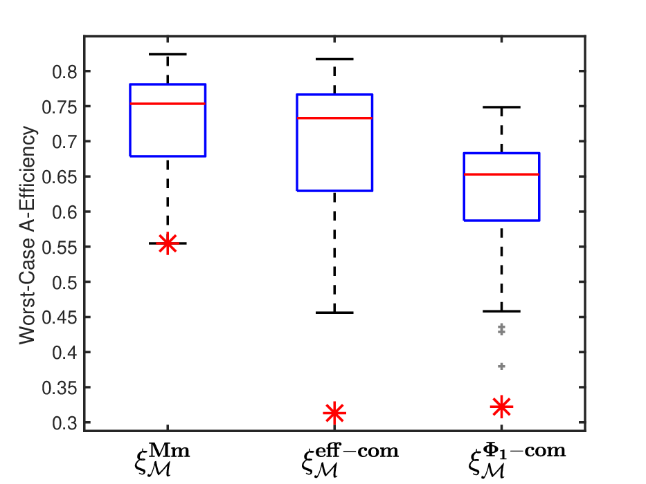
To compare the designs, we use the -efficiency defined in (2.4) as a larger-the-better performance measure. In particular, we consider (i.e., ) which is the D-optimality and which is the A-optimality. For each model space, we compute the -efficiency in (2.4) of all three designs relative to the corresponding local optimal design, and the local optimal design is obtained by the algorithm of Li and Deng 2018. For each model space, we can calculate the worse-case efficiency as .

| Worst-Case A-Efficiency | Worst-Case D-Efficiency | |||
|---|---|---|---|---|
| Mm- Design | 0.55 | 0.75 | 0.68 | 0.86 |
| Eff-Compromise Design | 0.31 | 0.73 | 0.58 | 0.85 |
| -Compromise Design | 0.32 | 0.65 | 0.55 | 0.82 |
Figure 1 shows the boxplot of the worst-case A- and D-efficiency of the Mm- design, eff-compromise design and -compromise design across 100 different model sets. The red asterisks “” in the boxplot denote the minimum worst-case A- and D-efficiency, and the larger the minimum, the better the design. Table 2 summarizes the minimum and median of the worst-case A- and D-efficiency of the three designs. The results show that the Mm- design returns the largest values on the minimum and median of the worst-case efficiency. We also notice that the eff-compromise design often gives the highest mean efficiency for a given model space, which is expected since it is designated to achieve the maximum mean efficiency. However, the mean A- and D-efficiency of all three designs are comparable on average over the 100 model sets. The computational times of Algorithm 1 to construct the Mm- design are about 7.59 seconds and 6.18 seconds for A- and D-optimality, respectively.
4.2 Uncertain Regression Coefficients
In the following Example 3, we further illustrate the advantages of Mm- design through an example considering the uncertain regression coefficients with the specified link function and basis functions . Note that when the regression coefficient space is continuous, a discretization is needed. In Example 3, the performance of the proposed design and algorithm over the unsampled values of regression coefficient is investigated.
Example 3. For a univariate logistic regression model with experimental domain and a quadratic basis, i.e. , consider a regression coefficient space . Since is continuous, we choose a Sobol sample of size twenty-six and the centroid of , i.e. , to form the surrogate coefficient set . Sobol sample is a low discrepancy sequence that converges to a uniform distribution on a bounded set and it is widely used in Monte Carlo methods (Sobol’ 1967). The surrogate model set is , where is the link function of the logistic regression. Four designs are considered: (1) Mm- design ; (2) eff-compromise design ; (3) local optimal design of the centroid of , i.e. , which can be viewed as either Mm- or compromise design with , and (4) Bayesian optimal design with uniform prior, which is also the -compromise design. Figure 2 shows the constructed designs under D- and A-optimality, respectively.
To compare the four designs, we use the -efficiency defined in (2.4) as a performance measure. Specifically, we generate a size of 10,000 Sobol sample from the original continuous region . For each of the sample, we compute the -efficiency in (2.4) of all four designs relative to the corresponding local optimal design, and the local optimal design is obtained in the same way as in Example 1. Figure 3 shows the boxplot of A- and D-efficiency of , , , and over 10,000 randomly sampled values. The red asterisks “” in the boxplot denote the worst-case A- and D-efficiency, and the larger the worst-case efficiency, the better the design. Table 3 summarizes the minimum and median A- and D-efficiency of the four designs.
It is seen that the Mm- design outperforms the other three designs in terms of the worst-case design efficiency, especially for A-optimality. Specifically, the worst-case A-efficiency of the Mm- design is 0.41, and is much larger than those of the other three designs. The worst-case D-efficiency of the Mm- design is 0.86 and is only slightly larger than those of other designs. We also found that the maximum A-efficiency of the Mm- design is the smallest, which is not surprising considering the Mm- design maximizes the worst-case efficiency, not the best-case efficiency.
To illustrate the computational efficiency of the proposed Algorithm 1, Figure 4 shows how the Mm- design criterion decreases with respect to the number of iterations. The computation times of Algorithm 1 to construct are 1.68 and 1.47 seconds for A- and D-optimality, respectively.


| A-Efficiency | D-Efficiency | |||
|---|---|---|---|---|
| Mm- Design | 0.41 | 0.70 | 0.86 | 0.98 |
| Eff-Compromise Design | 0.21 | 0.71 | 0.83 | 0.98 |
| Centroid Optimal Design | 0.16 | 0.71 | 0.81 | 0.98 |
| Bayesian Optimal Design | 0.26 | 0.69 | 0.84 | 0.98 |


4.3 Potato Packing Example
We consider a real-world example, the potato packing example in Woods et al. 2006, to further evaluate the proposed Mm- design. The experiment contains quantitative variables - vitamin concentration in the prepackaging dip and the amount of two kinds of gas in the packing atmosphere. The response is binary representing the presence or absence of liquid in the pack after 7 days. The basis functions of the logistic regression model always include the linear and quadratic terms of the input variables. But one set of the basis functions contains the interaction terms and the other one does not. The estimates of regression coefficients from a preliminary study in Woods et al. 2006 are given in Table 5 in the Appendix. Since enhancing prediction accuracy is a major goal for the experiment, we use the prediction-oriented I-optimality (Atkinson 2014) to evaluate the design efficiency. Note that the I-optimality shares the same mathematical structure as -optimality. The design points of the designs are shown in Figure 5 in the Appendix. Table 4 summarizes the I-efficiency of the Mm- design, eff-compromise design, and I-compromise design of the three potential model specifications. In terms of worst-case efficiency (i.e., smallest value of I-efficiency among , and ), the proposed Mm- design outperforms the other two designs by a large margin.
| Mm- Design | 0.64 | 0.71 | 0.82 |
|---|---|---|---|
| Eff-Compromise Design | 0.52 | 0.78 | 0.92 |
| I-Compromise Design | 0.49 | 0.80 | 0.92 |
5 Discussion
In this article, we proposed a new maximin -efficiency criterion Mm- for GLMs that aims at maximizing the worst-case design efficiency when various kinds of model uncertainties are considered, including uncertainties in link function, linear predictor and regression coefficients. An efficient algorithm to construct the Mm- design is also developed based on sound theoretical properties of the criterion. The proposed Mm- design and the algorithm can be easily extended to a more general case such as nonlinear models in Yang et al. 2013.
There are several directions for further research to enhance the proposed Mm- design and algorithm. First, to construct the Mm- design, one needs to form a set of possible model specifications. An interesting direction is how to extend the proposed design when such information of model specifications is limited or unavailable. Second, it is interesting to rigorously establish the convergence property of the optimal-weight procedure (Algorithm 2), which requires developing some other mathematical results. Third, the use of log-sum-exp approximation can be applied to other maximin design with a convex design criterion, and the theoretical and algorithmic developments can be adapted similarly. We plan to extend the framework to the more general setting for other maximin designs with convex criterion.
References
- Amzal et al. (2006) Amzal, B., Bois, F. Y., Parent, E., and Robert, C. P. (2006), “Bayesian-Optimal Design via Interacting Particle Systems,” Journal of the American Statistical Association, 101, 773–785.
- Atkinson (2014) Atkinson, A. C. (2014), “Optimal Design,” Wiley StatsRef: Statistics Reference Online, 1–17.
- Atkinson et al. (2006) Atkinson, A. C., Donev, A. N., and Tobias, R. D. (2006), Optimum Experimental Designs, with SAS, Oxford University Press.
- Atkinson and Woods (2015) Atkinson, A. C. and Woods, D. C. (2015), “Designs for generalized linear models,” Handbook of Design and Analysis of Experiments, 471–514.
- Burghaus and Dette (2014) Burghaus, I. and Dette, H. (2014), “Optimal designs for nonlinear regression models with respect to non-informative priors,” Journal of Statistical Planning and Inference, 154, 12–25.
- Calafiore and El Ghaoui (2014) Calafiore, G. C. and El Ghaoui, L. (2014), Optimization models, Cambridge university press.
- Dean et al. (2015) Dean, A., Morris, M., Stufken, J., and Bingham, D. (2015), Handbook of design and analysis of experiments, vol. 7, CRC Press.
- Dror and Steinberg (2006) Dror, H. A. and Steinberg, D. M. (2006), “Robust experimental design for multivariate generalized linear models,” Technometrics, 48, 520–529.
- Fedorov and Leonov (2013) Fedorov, V. and Leonov, S. (2013), Optimal Design for Nonlinear Response Models, Chapman & Hall/CRC Biostatistics Series.
- Fellman (1974) Fellman, J. (1974), On the Allocation of Linear Observations, Societas Scientiarum Fennica.
- Fiacco and Kortanek (1983) Fiacco, A. V. and Kortanek, K. O. (eds.) (1983), A Moment Inequality and Monotonicity of an Algorithm.
- Grant et al. (2009) Grant, M., Boyd, S., and Ye, Y. (2009), “cvx users? guide,” online: http://www. stanford. edu/˜ boyd/software. html.
- Imhof and Wong (2000) Imhof, L. and Wong, W. K. (2000), “A graphical method for finding maximin efficiency designs,” Biometrics, 56, 113–117.
- Khuri et al. (2006) Khuri, A. I., Mukherjee, B., Sinha, B. K., and Ghosh, M. (2006), “Design issues for generalized linear models: A review,” Statistical Science, 376–399.
- Kiefer (1974) Kiefer, J. (1974), “General equivalence theory for optimum designs (approximate theory),” The annals of Statistics, 849–879.
- Kiefer (1985) — (1985), “Optimal Design: Variation in Structure and Performance Under Change of Criterion,” Biometrika, 62, 277–288.
- King and Wong (1998) King, J. and Wong, W. K. (1998), “Optimal minimax designs for prediction in heteroscedastic models,” Journal of Statistical Planning and Inference, 69, 371–383.
- King and Wong (2000) King, J. and Wong, W.-K. (2000), “Minimax D-optimal designs for the logistic model,” Biometrics, 56, 1263–1267.
- Li and Majumdar (2009) Li, G. and Majumdar, D. (2009), “Some results on D-optimal designs for nonlinear models with applications,” Biometrika, 96, 487–493.
- Li and Deng (2018) Li, Y. and Deng, X. (2018), “An Efficient Algorithm for Elastic I-optimal Design of Generalized Linear Models,” arXiv preprint arXiv:1801.05861.
- Schwabe (1997) Schwabe, R. (1997), “Maximin efficient designs Another view at D-optimality,” Statistics & probability letters, 35, 109–114.
- Silvey (2013) Silvey, S. D. (2013), Optimal design: an introduction to the theory for parameter estimation, vol. 1, Springer Science & Business Media.
- Silvey et al. (1978) Silvey, S. D., Titterington, D. M., and Torsney, B. (1978), “An algorithm for optimal designs on a finite design space,” Communications in Statistics - Theory and Methods, 14, 1379–1389.
- Sitter (1992) Sitter, R. R. (1992), “Robust designs for binary data,” Biometrics, 1145–1155.
- Sitter and Torsney (1995) Sitter, R. R. and Torsney, B. (1995), “D-Optimal Designs for Generalized Linear Models,” in MODA4 — Advances in Model-Oriented Data Analysis, eds. Kitsos, C. P. and Müller, W. G., Heidelberg: Physica-Verlag HD, pp. 87–102.
- Sobol’ (1967) Sobol’, I. M. (1967), “On the distribution of points in a cube and the approximate evaluation of integrals,” Zhurnal Vychislitel’noi Matematiki i Matematicheskoi Fiziki, 7, 784–802.
- Waite and Woods (2015) Waite, T. W. and Woods, D. C. (2015), “Designs for generalized linear models with random block effects via information matrix approximations,” Biometrika, 102, 677–693.
- Wong (1992) Wong, W.-K. (1992), “A unified approach to the construction of minimax designs,” Biometrika, 79, 611–619.
- Wong and Cook (1993) Wong, W. K. and Cook, R. D. (1993), “Heteroscedastic G-optimal designs,” Journal of the Royal Statistical Society: Series B (Methodological), 55, 871–880.
- Wong et al. (2019) Wong, W. K., Yin, Y., and Zhou, J. (2019), “Optimal Designs for Multi-Response Nonlinear Regression Models With Several Factors via Semidefinite Programming,” Journal of Computational and Graphical Statistics, 28, 61–73.
- Woods and Lewis (2011) Woods, D. C. and Lewis, S. M. (2011), “Continuous optimal designs for generalized linear models under model uncertainty,” Journal of Statistical Theory and Practice, 5, 137–145.
- Woods et al. (2006) Woods, D. C., Lewis, S. M., Eccleston, J. A., and Russell, K. (2006), “Designs for generalized linear models with several variables and model uncertainty,” Technometrics, 48, 284–292.
- Woods et al. (2017) Woods, D. C., Overstall, A. M., Adamou, M., and Waite, T. W. (2017), “Bayesian design of experiments for generalized linear models and dimensional analysis with industrial and scientific application,” Quality Engineering, 29, 91–103.
- Wu and Stufken (2014) Wu, H.-P. and Stufken, J. (2014), “Locally -optimal designs for generalized linear models with a single-variable quadratic polynomial predictor,” Biometrika, 101, 365–375.
- Yang et al. (2013) Yang, M., Biedermann, S., and Tang, E. (2013), “On Optimal Designs for Nonlinear Models: A general and Efficient Algorithm,” Journal of the American Statistical Association, 108, 1411–1420.
- Yang and Stufken (2009) Yang, M. and Stufken, J. (2009), “Support points of locally optimal designs for nonlinear models with two parameters,” The Annals of Statistics, 37, 518–541.
- Yang and Stufken (2012) — (2012), “Identifying Locally Optimal Designs for Nonlinear Models: A Simple Extension with Profound Consequences,” The Annals of Statistics, 40, 1665–1681.
- Yang et al. (2011) Yang, M., Zhang, B., and Huang, S. (2011), “Optimal designs for generalized linear models with multiple design variables,” Statistica Sinica, 1415–1430.
- Yu (2010) Yu, Y. (2010), “Monotonic Convergence of a General Algorithm for Computing Optimal Designs,” The Annals of Statistics, 38, 1593–1606.
Department of Mathematical Sciences, DePaul University, Chicago, IL
E-mail: yli139@depaul.edu
Department of Applied Mathematics, Illinois Institute of Technology, Chicago, IL
E-mail: lkang2@iit.edu
Department of Statistics, Virginia Tech, Blacksburg, VA
E-mail: xdeng@vt.edu
6 Appendix
Lemma 1.
defined in (2.9) is a convex function of design .
Proof.
Since is convex with respect to (Yang and Stufken 2012) and is a convex and strictly increasing function, the composite function is a convex function of . As a result, is a convex function of . ∎
Lemma 2.
The directional derivative of in the direction from to is
where
Proof.
Lemma 3.
The directional derivative of in the direction of a single point is given as,
where .
Particularly, the directional derivatives of D-, A- and the prediction-oriented criterion EI-optimality defined in (Li and Deng 2018) are:
where for EI-optimality is pre-determined and it does not depend on the design . The cdf is the user-specified distribution for the EI-optimality.
Lemma 4.
For a design with fixed design points , in (2.11) is a convex function with respect to the weight vector .
Proof.
The proof is similar to that of Lemma 1. ∎
Proof of Theorem 1
Proof.
- i.
: As is a convex function in proved in Lemma 1, the directional derivative holds for any , and the inequality becomes equality if is a support point of the design .
- ii.
: If holds for any , then minimizes as is a convex function in .
∎
Proof of Lemma 5
Proof.
The lemma is proved for the case, and the case could be proved similarly. The directional derivative of in the direction of the point is:
for any , where denotes the information matrix of the design with a unit mass on single point .
Denote the Mm- design . With (6), we have
| (6.21) | |||||
Furthermore, with the definition of directional derivative in the direction of the Mm- design and convexity of , we have
| (6.22) | |||||
Proof of Theorem 2
Proof.
When , holds automatically.
When , that is, , define , then it follows immediately from Lemma 5 that
| (6.23) |
Since the function is an increasing function of , because of its definition and , we have
Thus, together with (6.23), . ∎
Proof of Theorem 3
Proof.
We show the proof for the scenario in the -criterion. The proof for could be done similarly. The proof is established by proof of contradiction. Suppose that the Algorithm 1 does not converge to the Mm- design , then we have
For any iteration , since and the Optimal-Weight Procedure returns optimal weight vector that minimizes criterion, the design cannot be worse than the design in the previous iteration , i.e.,
Thus, for all , there exists , such that,
According to Lemma 5,
for any . Then, the Taylor expansion of is upper bounded by
| (6.24) | |||||
where is the second-order directional derivative of evaluated at a value between 0 and .
For Algorithm 1, the criterion is minimized, for all we have
or equivalently,
As a result, , which contradicts with the fact that for any design . Thus,
Since on is a continuous function,
∎
Description of Algorithm 2.
There are three user-specified parameters , , and in Algorithm 2. is the tolerance of convergence, and we usually set it to be . is the maximum number of iterations and we set it to be in all numerical examples. The parameter plays the same role as in the classical multiplicative algorithm (Silvey et al. 1978), which is to control the speed of the convergence. According to the numerical study by Fellman 1974 and Fiacco and Kortanek 1983, is often chosen as 1 for D-optimality, and 0.5 for A- or EI-optimality.
Derivation of (4) is stated as follows. Update the weight of in iteration with
| (6.29) |
then normalize the weights to ensure the sum 1 condition as
| (6.30) |
Additional Tables and Figures for Section 4.3.
| Term | First-Order | With interaction | Second-order |
|---|---|---|---|
| Intercept | -0.28 | -1.44 | -2.93 |
| 0 | 0 | 0 | |
| -0.76 | -1.95 | -0.52 | |
| -1.15 | -2.36 | -0.79 | |
| 0 | 0 | ||
| 0 | 0 | ||
| -2.34 | -0.66 | ||
| 0.94 | |||
| 0.79 | |||
| 1.82 |
