Observation of high-order Mollow triplet by quantum mode control with concatenated continuous driving
Abstract
The Mollow triplet is a fundamental signature of quantum optics, and has been observed in numerous quantum systems. Although it arises in the “strong driving” regime of the quantized field, where the atoms undergo coherent oscillations, it can be typically analyzed within the rotating wave approximation. Here we report the first observation of high-order effects in the Mollow triplet structure due to strong driving. In experiments, we explore the regime beyond the rotating wave approximation using concatenated continuous driving that has less stringent requirements on the driving field power. We are then able to reveal additional transition frequencies, shifts in energy levels, and corrections to the transition amplitudes. In particular, we find that these amplitudes are more sensitive to high-order effects than the frequency shifts, and that they still require an accurate determination in order to achieve high-fidelity quantum control. The experimental results are validated by Floquet theory, which enables the precise numerical simulation of the evolution and further provides an analytical form for an effective Hamiltonian that approximately predicts the spin dynamics beyond the rotating wave approximation.
I Introduction
The Mollow triplet was originally observed in coupled atom-laser systems, where the laser field creates a series of equidistant energy level manifolds and induces the coupling inside each manifold Mollow 1969. The coherent atomic oscillations modulate the laser driving field and spontaneous emission acts as a detection tool for the triplet energy levels Cohen-Tannoudji 1996. The Mollow triplet structure has been observed in atomic beams Schrama et al. 1992, ions Stalgies et al. 1996, single molecules Wrigge et al. 2008, quantum dots Nick Vamivakas et al. 2009; Flagg et al. 2009; Peiris et al. 2015; Lagoudakis et al. 2017, superconducting qubits Baur et al. 2009, and cold atoms Ortiz-Gutiérrez et al. 2019. Its potential applications, such as heralded single-photon sources Ulhaq et al. 2012, quantum sensing Joas et al. 2017; Stark et al. 2017; Hönigl-Decrinis et al. 2020, and spin noise characterization Poshakinskiy and Tarasenko 2020, make it a versatile tool in physics.
Even an electromagnetic field in the microwave range, such as in magnetic resonance experiments, can produce a similar level structure. Typical Larmor precession under a single (classical) microwave driving (Rabi oscillation) is not able to reveal the Mollow triplet since the observation operator commmutes with the static splitting . By applying multiple driving fields to orient the effective static splitting Hamiltonian along a transverse direction, it becomes possible to observe the Mollow triplet by Rabi oscillation, as observed in nitrogen-vacancy (NV) centers in diamond Rohr et al. 2014; Teissier et al. 2017; Pigeau et al. 2015.
In previous experiments Schrama et al. 1992; Stalgies et al. 1996; Wrigge et al. 2008; Nick Vamivakas et al. 2009; Flagg et al. 2009; Peiris et al. 2015; Lagoudakis et al. 2017; Baur et al. 2009; Ortiz-Gutiérrez et al. 2019; Rohr et al. 2014; Teissier et al. 2017; Pigeau et al. 2015 that showed the Mollow triplet, the driving strength was smaller than the static splitting, allowing one to conveniently solve the dynamics using the rotating wave approximation (RWA). Previous theoretical studies beyond the RWA have predicted frequency shifts and imbalanced sidebands Lü and Zheng 2012; Yan et al. 2013, yet experimental verification is still lacking due to the limited driving strength. The aim of this paper is to experimentally explore the Mollow triplet structure in the regime beyond the RWA.
To overcome the usual constraints on the driving power needed to achieve the strong driving regime beyond the RWA, we use concatenated continuous driving (CCD). CCD is a continuous dynamical decoupling technique with multiple resonant modulated fields, and has been studied before in the context of qubit coherence protection Cai et al. 2012; Khaneja et al. 2016; Saiko et al. 2018; Cohen et al. 2017; Farfurnik et al. 2017; Rohr et al. 2014; Layton et al. 2014; Saiko et al. 2015; Teissier et al. 2017; Bertaina et al. 2020; Cao et al. 2020; Wang et al. 2020. As we show below, in the first interaction picture, the CCD driving term generates a Hamiltonian describing the typical AC driving of a two-level system, although with the static field along the x direction Rohr et al. 2014; Teissier et al. 2017; Pigeau et al. 2015; Wang et al. 2020. Then, since the static energy in the first interaction picture is set by the Rabi frequency, the ratio of the driving to the static splitting can be made much larger than in typical Rabi experiments Cohen et al. 2017; Farfurnik et al. 2017; Laucht et al. 2016; Wang et al. 2020. In addition, the initial state does not commute with the interaction picture transformation, which makes it possible to observe the Mollow triplet by Rabi oscillation. Thus, CCD is a good experimental tool to study novel physics beyond the RWA, and in particular, the Mollow triplet.
To analyze our experimental results, we use Floquet theory as a precise numerical tool to solve the evolution as a summation of a series of modes. To gain further insight, we also use Floquet theory as an analytical way to evaluate the effective Hamiltonian and calculate the corrections to frequency values and transition amplitudes resulting from the strong driving. We can thus provide a complete picture of the Mollow triplet structure beyond the rotating wave approximation.
II Mollow triplet with CCD

Here we introduce the CCD scheme and show how it can be used to reveal the Mollow triplet. We study a two-level system with a static splitting along z, coupled to an amplitude-modulated microwave applied along the x axis given by . When the RWA condition is satisfied, by going into the first rotating frame defined by and neglecting the counter-rotating term, the Hamiltonian becomes
| (1) |
where is the frequency detuning. Figure 1(a) shows the static and oscillating fields in the lab and first rotating frames. A similar Hamiltonian can also be engineered by phase modulation, where the phase of the microwave is modulated as and the Hamiltonian in the interaction picture becomes
| (2) |
Evolution under the CCD Hamiltonian in Eq. (1) can be solved with a second interaction picture defined by with and . When and , by dropping the counter-rotating terms, the Hamiltonian in the second interaction picture becomes
| (3) |
The spin evolution in the first rotating frame is simply , where modulates the dynamics happening in the second rotating frame. Then, we expect that the population in to be generally a sum over the three frequencies , , where in the RWA (see Supplemental Material). Since the population measurement is along a direction that does not commute with the second interaction picture transformation along , the Mollow triplet structure can be revealed by the CCD scheme Rohr et al. 2014; Teissier et al. 2017; Pigeau et al. 2015.
While this standard RWA description provides a simple analytical solution to the dynamics, using Floquet theory (see Appendix A) provides further insight about the energy level structure, in analogy to the quantized field picture typically used to analyze the Mollow triplet in atomic physics. Similar to the dressed atom approach Cohen-Tannoudji 1996 where a series of equidistant level manifolds form the energy structure (see Fig. 1(b)), Floquet theory also predicts a series of energy manifolds Chu and Telnov 2004, , separated by integer-spacings of , where are the eigenenergies obtained by solving the Floquet Hamiltonian . Within the RWA, the Floquet Hamiltonian is block-diagonal Shirley 1965. The off-diagonal terms in each block induce transitions between two adjacent level manifolds separated by . The system-field coupling modifies the splitting by , which creates the Mollow triplet structure with a center band at and two sidebands at . The dressed state energy difference within the RWA is , where is the effective Rabi frequency. Going beyond the RWA allows one to observe a richer framework of dynamics that we explore in the following.
Our device is based on NV ensembles used in Ref. Jaskula et al. 2019 with spins being addressed simultaneously. Two NV electronic spin states and with a splitting are used as the logical and . An arbitrary waveform generator creates the modulated waveform to engineer the CCD Hamiltonian. By driving the NV centers with the amplitude-modulated CCD scheme, we observe the Mollow triplet in the Fourier spectra of the NV Rabi oscillations (see Figs. 1(c) and 1(d)). In particular, we have phase control over the waveform, can separately observe the center band (spin-locking condition) as well as the sidebands, and carefully investigate their behavior.
III High-order Mollow triplet
Previous work has explored novel phenomena caused by strong driving, such as the Bloch-Siegert shift Bloch and Siegert 1940; Ahmad and Bullough 1974, Landau-Zener-Stückelberg interference Shevchenko et al. 2010; Huang et al. 2011, coherent destruction of tunneling (CDT) Grossmann et al. 1991; Grossmann et al. 1993, novel behaviors in the quantum Zeno and anti-Zeno effects Zheng et al. 2008; Ai et al. 2010, and asymmetric spectral features of the Mollow triplet Yan et al. 2013. Here we theoretically and experimentally study the high-order Mollow triplet structure induced by strong driving, including corrections to energy levels and transition amplitudes.
To analyze our experimental results, we use Floquet theory which is known to accurately predict the system dynamics, including high-order phenomena, due to the counter-rotating terms beyond the RWA. Floquet theory describes the periodic Hamiltonian as a time-independent operator in Fourier space. One can then numerically calculate the evolution by truncating the (infinite) Floquet matrix Leskes et al. 2010; Shirley 1965. Due to the simplicity of the computation, we perform a truncation to the Floquet matrix to high order ( blocks) to accurately calculate the evolution. Analytical approximations in various parameter ranges are also possible, either by moving to a suitable interaction picture where on-resonance terms highlight the corrections to the Hamiltonian due to the counter-rotating terms Ashhab et al. 2007; Yan et al. 2015; Yan et al. 2014; Yan et al. 2013; Lü and Zheng 2012; Zhou et al. 2014, or by iteratively block-diagonalizing the time-independent Floquet Hamiltonian with a unitary transformation Leskes et al. 2010. In addition to providing numerical and approximate solution model, the Floquet picture, with its ladder-like energy structure, also provides an insightful understanding of the dynamics, in analogy to transitions and hoppings between energy levels in the dressed atom approach Cohen-Tannoudji 1996; Chu and Telnov 2004. Floquet theory can then be used as a tool to engineer desired Hamiltonian interactions, with applications relevant for areas from many-body systems to quantum control Eckardt 2017; Childs et al. 2018.
When applied to a two-level system, Floquet theory predicts a series of energy level manifolds yielding three types of transition frequencies (modes), , (see Appendix. A). The exact evolution is a superposition of two Floquet eigenstates and the ensuing Rabi oscillation is a sum over these components, where denotes the th triplet with , and the transition amplitudes are obtained from Floquet theory. can be tuned by varying the initial conditions and the driving phase. This allows for control over the frequency modes involved in the evolution (mode control).
A single mode evolution with only frequency components can be achieved when the initial state is one of the two eigenstates and , which is equivalent to a spin-locking condition. In the RWA case, only components with can be observed in the Mollow triplet. However, when the counter-rotating terms in the Floquet matrix are not negligible, frequency components with emerge (see Appendix A). At the same time, values of the energy level and transition amplitudes will both deviate from the RWA predictions.
In the following, we analyze the corrections to the energy levels and transition amplitudes. The Floquet approach can be used to analytically derive an effective, approximate Hamiltonian by systematically including higher order corrections beyond the RWA. By applying the van Vleck transformation Leskes et al. 2010, a unitary transformation to block-diagonalize the Floquet Hamiltonian, we obtain the effective Hamiltonian up to first order correction in the second rotating frame
| (4) |
where is the correction term and we assumed so that and the correction term is along x. Under the resonance condition , the shift of the level splitting inside each energy manifold is with which quadratically depends on the ratio . The direction of the effective microwave field deviates from the y axis by a small angle within the XY plane. Such a linear dependence on induces drastic changes of the transition amplitudes . The amplitude of each frequency component can be found analytically using the Hamiltonian in Eq. (4), yielding a shift with respect to the RWA results. The amplitude shift of the th frequency component, , depends on the initial state : for the central band, when is perpendicular to both the driving direction y and the Hamiltonian correction direction x; when is along the driving direction y; and when is along x. For the sidebands, in all three scenarios, the shifts are linear in , with corresponding to the two sidebands. Ultimately, the existence of the correction term breaks the symmetry of the two sidebands under the resonant condition and results in large changes of the transition amplitudes especially for the sidebands. In comparison, the energy level correction is less sensitive to the counter-rotating effects.
III.1 Sideband asymmetry

We implement amplitude-modulated CCD experiments to systematically study the evolution mode control under the resonance condition , with . By applying a strong oscillating field, , we are able to observe the sideband asymmetry and the eigenstate shifts predicted by the theoretical analysis above. We implement mode control by sweeping the phase of the driving, or the angle of the initial states in the ZY plane (see also Appendix Fig. 6 for results obtained when sweeping the initial state direction in the XY and XZ planes). The corresponding Rabi oscillations are measured by projecting the time-dependent state onto . The FFT spectrum of the Rabi oscillations and the fitted transition amplitudes are plotted in Fig. 2.
Neglecting the counter-rotating terms (dashed lines), the two sidebands have the same amplitudes for both the phase and initial state sweeps. However, experimentally, we measure a large asymmetry in the sideband amplitudes, with different asymmetry for the phase sweep and the initial state sweep. Such an effect can be explained by the correction term in the Hamiltonian in Eq. (4) which makes the eigenstate shift from the y axis in the XY plane, introducing a dissimilarity between the phase and initial state sweeps. In the initial state sweep, a single mode evolution is achieved when the initial state is prepared along a shifted direction (see Fig. 6(d) in Appendix). Tuning only the phase cannot instead achieve such a single mode evolution. Experiments show that the amplitudes of the sidebands deviate from the RWA prediction throughout all the ranges in Figs. 2(c) and 2(d). The amplitude of the center band only has a large deviation from the RWA prediction when the initial state is close to the driving direction y in the ZY sweep in (d) with . When the initial state is far away from the y direction, the Floquet prediction overlaps with the RWA prediction. The initial state sweep experiments in Fig. 2 and in Appendix Fig. 6 show that for the center band, , as predicted from the analysis, where denote the corresponding directions of the initial state. Whereas analysis with the effective Hamiltonian in Eq. (4) only provides a qualitative estimate, Floquet simulation accurately predicts the values of the amplitudes quantitatively for all experimental conditions.
In addition to frequency and amplitude shifts, we see frequency components and even appearing in the range of . Even though their intensities are weak, these frequency components represent results that are beyond those predicted by the RWA.
Thus, large deviation from the RWA predictions happens in the evolution mode control experiments, indicating drastic modifications caused by the counter-rotating terms. One application of the CCD scheme is to protect quantum information by tuning the evolution mode to the robust center band when the spin-locking condition is satisfied. Our experiment shows that such a condition is shifted and a simple phase adjustment is not enough to find the optimal condition when the driving strength is comparable with the static splitting. One solution is to tune the driving strength to compensate for the Hamiltonian correction, as discussed in the following subsection.
III.2 Resonance shifts

Without the counter-rotating effect, in the first rotating frame (see Eq. (1)), the resonance condition is satisfied when (). We study the resonance shift caused by counter-rotating effects by experimentally sweeping the main driving strength under two different modulation phases (see Figs. 3(a) and 3(c)). The frequency shifts due to counter-rotating terms are very small when . A larger shift appears when , and the Floquet prediction plotted with dashed red and light blue lines in Figs. 3(a) and 3(c) showcases an improved fit on the experimental data. Figures 3(b) and 3(d) are the oscillation amplitudes of the corresponding frequency components obtained by fitting the Rabi oscillation data. The Floquet predictions are plotted in solid lines while the RWA predictions are plotted in dashed lines. When , the disappearance of the sidebands happens at in (d), which is clearly on the left of the resonant frequency , indicating a change of the resonance condition. Similarly, when , the crossing point of the two sidebands is also at in (b). In Eq. (4), the detuning term can be seen as a compensation of the correction . A simple calculation predicts the compensation at , which is still larger than the measured and simulated values of , indicating that just including the first order correction in the effective Hamiltonian in Eq. (4) is not enough, and more corrections need to be taken into account. The Floquet calculation is an accurate way to predict such a shift. Note that when is small, the measured amplitudes are lower than the theoretical curve: this is due to the small Rabi contrast under weak driving (see details in Supplemental Material).
In addition to the resonance shifts, we also observe higher-order frequency components corresponding to in the Mollow triplet. In Figs. 3(a) and 3(c), we use the dashed red and light blue lines to plot the first (n=1) and second set (n=2) of frequency values of the Mollow triplet predicted by the Floquet theory. In Fig. 3(c), we clearly observe the and components when is small. In Fig. 3(a), we see the sidebands of the set around and the sidebands with also exist but are partly hidden under the dashed lines.
III.3 Frequency shifts and avoided crossing

Since the energy eigenvalues are less sensitive to the counter-rotating effects, a larger driving strength is needed to observe a frequency deviation from the RWA predictions. We swept the modulation strength from 0 to in the phase-modulated CCD scheme, on resonance and for two different driving field phases (). The FFT spectra of the measured Rabi oscillations are plotted in Figs. 4(a) and 4(c), while Figs. 4(b) and 4(d) show the equivalent spectra simulated by the Floquet approach. We further compare the simulations to the predictions based on the RWA (red dashed lines). When , three frequency components dominate the spectra. Within this region, both the Floquet and the RWA approaches correctly predict the frequencies of the three bands in the Mollow triplet structure, with the two sidebands linearly dependent on . When becomes larger, a pattern appears in the higher frequency region corresponding to the third manifold of the Mollow triplet structure centered at , which follows a simple translation of the lowest order pattern centered at . In our experiments, we can thus clearly observe at least two higher order Mollow triplets as predicted by Floquet simulations, in addition to the one predicted by the RWA. Note that the two sidebands frequencies are no longer linearly dependent on and display a clear bending around 4.8MHz due to an avoided crossing. We show in Fig. 5 in Appendix that such avoided crossings are caused by the mixing between the frequency components and due to the counter-rotating terms. Such an avoided crossing only exists in the Floquet simulation.
IV Conclusion
In this work, we explored higher order effects in the Mollow triplet structure by experimentally applying a modulated driving field (following the CCD scheme) and analyzing the results with Floquet theory. We observed frequency components beyond the RWA predictions, shifts of the eigenenergies and of the transition amplitudes . Our results not only demonstrate the ability of the modulated driving protocol to observe effects due to the strong driving, but also pave the way to employing this technique for robust control. Indeed, as the frequency components of the Floquet evolution are only determined by the modulation frequency , they are robust against external noise and fluctuations in the driving fields. Combined with our mode-control technique, this enables the generation of highly-robust quantum states Wang et al. 2020. Nevertheless, to achieve such robustness, a precise knowledge of the Floquet eigenstates is needed to accurately select the initial state or the driving phase, as demonstrated by our experimental results. Thus, insights from Floquet theory can be used to design robust quantum operations and protect the quantum coherence Wang et al. 2020. In particular, our work shows that to achieve optimal quantum control with the CCD scheme, we should be careful of not only the eigenenergy shifts due to the counter-rotating terms, but also the amplitude changes and resonance shifts, both of which prove to be more sensitive. Beyond applications to robust quantum control, our results provide a versatile technique for studying the effects of strong driving, overcoming practical experimental limitations in reaching the strong-driving regime, that could be applied to investigate other phenomena such as coherent destruction of tunneling and dynamic localization.
Acknowledgement
This work was supported in part by DARPA DRINQS and NSF PHY1915218. We thank Pai Peng for fruitful discussions and Thanh Nguyen for manuscript revision.
Appendix A Floquet theory
Floquet theory can be used to solve the quantum dynamics under a Hamiltonian periodic in time Shirley 1965. Similar to Bloch theory which can solve a Hamiltonian periodic in space and gives rise to a series of band structures in k-space, Floquet theory also predicts a series of ’band’ structures in frequency space. Although the principles of Floquet theory is simple and straightforward, the physics residing in its energy structure equips it with the ability to solve detailed dynamics of higher order phenomena such as multi-photon process Chu and Telnov 2004. Given a time-periodic Hamiltonian , the wavefunction has the form where is periodic in time and denotes the eigenenergy of the system. To solve for the wavefunction time evolution, we can apply the following steps. (1) Decompose the Hamiltonian and the state vector into a Fourier series and . (2) Write out the Floquet matrix (see Eq. (7)). (3) Solve for the eigenvalue problem of the Floquet matrix . (4) Apply the initial conditions to get the coefficients of each eigenstate . (5) Obtain the evolution . Below we explicitly show how to implement this procedure.
A.1 General derivation of Floquet theory
To solve the Schrödinger equation , we obtain the eigenvalue problem for the periodic part ,
| (5) |
Plugging in the Fourier expansions , we obtain
| (6) |
Writing out equation above in matrix form, we obtain
| (7) |
where the matrix in Eq. (7) is the Floquet matrix .
By solving for the eigenenergies and eigenvectors of the Floquet matrix, one can find the time-dependent energy eigenvectors of the system . The evolution of the system can then be expressed as a superposition of these eigenvectors
| (8) |
with coefficients determined by the initial condition
| (9) |
.
Quasi energy
If is the eigenenergy of the system, for any integer n is also the eigenenergy of the system since . The eigenfunction for the eigenenergy is the same as the eigenfunction for the eigenenergy . As a result, it is usually possible to limit the range of the eigenvalues within the first “Brillouin zone” since all eigenvalues in the other zones will be a simple (frequency) translation of the values in the first zone.
Number of solutions in a two level systems
For two level systems, the Hamiltonian can be written as a matrix. The wavefunction , its periodic part , and the Fourier components , are two dimensional vectors. Thus, there are only two non-trivial solutions denoted by .
A.2 Concatenated continuous driving
We consider the Hamiltonian of the amplitude-modulated concatenated continuous driving in the interaction picture . Fourier decomposition of Hamiltonian gives . Applying the Floquet approach to solve for the exact evolution of the system we obtain the following eigenvalue equation
| (10) |
The evolution of the system can be written in terms of the Floquet energy eigenvalues and eigenvectors, taking into account the initial conditions:
| (11) |
The system evolution is probed experimentally by measuring the system population by projecting the state onto . The probability of being in the state presents three classes of frequencies: and , with integer:
| (12) | ||||
We can rewrite this expression as
| (13) |
with , where , , and The first few frequencies and coefficients are listed in Table 1.
| Frequency | Coefficients |
|---|---|
| 0 | |
When the RWA is valid, , and the resonant condition is satisfied, counter-rotating terms can be dropped yielding a block-diagonal Floquet Hamiltonian. (Note that a frame transformation that aligns the static field along z and the oscillating field along x is needed to obtain this block-diagonal form.) Following such procedure gives , where and the only non-vanishing oscillating components in the population are the first five components listed in Table 1. When the approximation is not valid, more frequency components are involved and the evolution is made more complicated.
A.3 Two definitions of
As discussed above, there are two nontrivial solutions for the Floquet matrix up to a translation of where n is any integer. One definition of is by limiting their values within the first zone , which is used in the numerical simulations in this work to simplify the calculation. An example of such a definition corresponding to Fig. 4 is shown in Fig. 5(a). In this paper, we use this definition for the amplitude calculation in Figs. 7(b) and 7(d) and Figs. 3(b) and 3(d) where we see a sudden switch between the frequency components and when . However, this definition makes it difficult to clarify whether we observe frequency components beyond the RWA. To clarify that we observe higher order frequency components with , we use a definition that has a correspondence to the prediction obtained from the analytical RWA approach and no longer limits the range of . Figure 5(b) shows such a definition where each manifold of Mollow triplet is clearly seen. In Figs. 7(a) and 7(c) and Figs. 3(a) and 3(c), the dashed lines are the frequency prediction from the Floquet theory using the same definition.
Appendix B Mode control of the evolution and resonance shifts
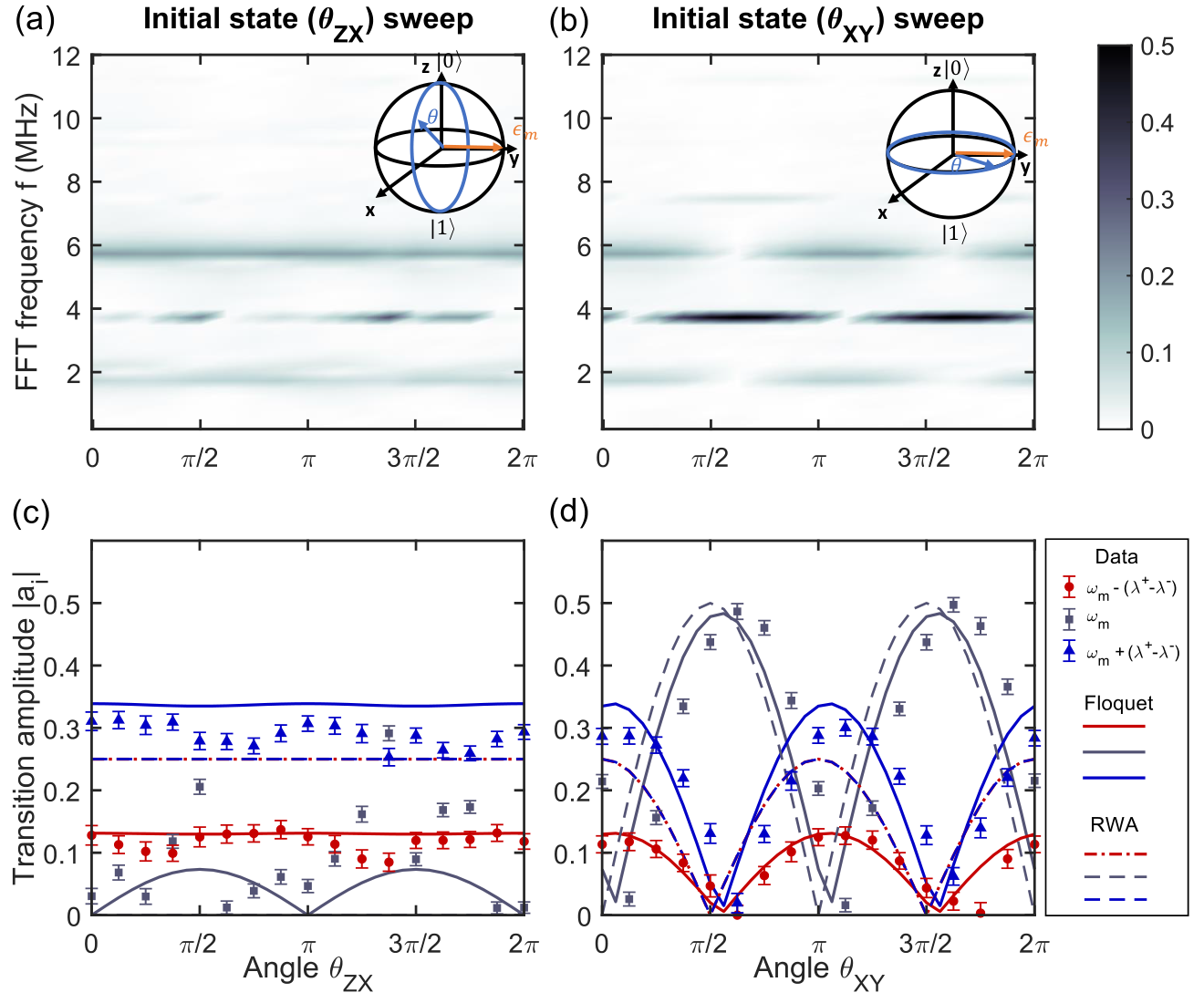
In the main text we demonstrate control of the system evolution by sweeping the driving phase and the initial state. This enables tuning the evolution to highlight different frequency modes. Here we provide additional demonstration of such mode control by sweeping the initial state in the ZX plane and XY plane (see Fig. 6). These results further highlight the need to take counter-rotating effects when describing the system evolution under strong driving.

As we increase the driving strength to observe these effects we reach the saturation limits of our apparatus. This leads to unwanted, albeit interesting, additional modulations of the dynamics.
We reproduce in Fig. 7 the results shown in the main text (Fig. 3) but in the Floquet simulations we do not take into account saturation effects due to imperfect electronics and power saturation of the amplifier. When we add an additional term to the Hamiltonian in Eq. (1) to mimic the saturation effects, we reproduce the gradual switch between frequency components at . Instead the Floquet simulation without any additional terms predicts that the switching happens suddenly at a single point (see Fig. 7 and Supplemental Material for more details on the power saturation and avoided crossings).
References
- Mollow (1969) B. R. Mollow, Physical Review 188, 1969 (1969).
- Cohen-Tannoudji (1996) C. N. Cohen-Tannoudji, in Amazing Light: A Volume Dedicated to Charles Hard Townes on His 80th Birthday, edited by R. Y. Chiao (Springer New York, New York, NY, 1996) pp. 109–123.
- Schrama et al. (1992) C. A. Schrama, G. Nienhuis, H. A. Dijkerman, C. Steijsiger, and H. G. M. Heideman, Physical Review A 45, 8045 (1992).
- Stalgies et al. (1996) Y. Stalgies, I. Siemers, B. Appasamy, T. Altevogt, and P. E. Toschek, Europhysics Letters (EPL) 35, 259 (1996).
- Wrigge et al. (2008) G. Wrigge, I. Gerhardt, J. Hwang, G. Zumofen, and V. Sandoghdar, Nature Physics 4, 60 (2008).
- Nick Vamivakas et al. (2009) A. Nick Vamivakas, Y. Zhao, C.-Y. Lu, and M. Atatüre, Nature Physics 5, 198 (2009).
- Flagg et al. (2009) E. B. Flagg, A. Muller, J. W. Robertson, S. Founta, D. G. Deppe, M. Xiao, W. Ma, G. J. Salamo, and C. K. Shih, Nature Physics 5, 203 (2009).
- Peiris et al. (2015) M. Peiris, B. Petrak, K. Konthasinghe, Y. Yu, Z. C. Niu, and A. Muller, Physical Review B 91, 195125 (2015).
- Lagoudakis et al. (2017) K. G. Lagoudakis, K. A. Fischer, T. Sarmiento, P. L. McMahon, M. Radulaski, J. L. Zhang, Y. Kelaita, C. Dory, K. Müller, and J. Vučković, Physical Review Letters 118, 013602 (2017).
- Baur et al. (2009) M. Baur, S. Filipp, R. Bianchetti, J. M. Fink, M. Göppl, L. Steffen, P. J. Leek, A. Blais, and A. Wallraff, Physical Review Letters 102, 243602 (2009).
- Ortiz-Gutiérrez et al. (2019) L. Ortiz-Gutiérrez, R. C. Teixeira, A. Eloy, D. Ferreira da Silva, R. Kaiser, R. Bachelard, and M. Fouché, New Journal of Physics 21, 093019 (2019).
- Ulhaq et al. (2012) A. Ulhaq, S. Weiler, S. M. Ulrich, R. Roßbach, M. Jetter, and P. Michler, Nature Photonics 6, 238 (2012).
- Joas et al. (2017) T. Joas, A. M. Waeber, G. Braunbeck, and F. Reinhard, Nature Communications 8, 964 (2017).
- Stark et al. (2017) A. Stark, N. Aharon, T. Unden, D. Louzon, A. Huck, A. Retzker, U. L. Andersen, and F. Jelezko, Nature Communications 8, 1105 (2017).
- Hönigl-Decrinis et al. (2020) T. Hönigl-Decrinis, R. Shaikhaidarov, S. de Graaf, V. Antonov, and O. Astafiev, Physical Review Applied 13, 024066 (2020).
- Poshakinskiy and Tarasenko (2020) A. V. Poshakinskiy and S. A. Tarasenko, Physical Review B 101, 075403 (2020).
- Rohr et al. (2014) S. Rohr, E. Dupont-Ferrier, B. Pigeau, P. Verlot, V. Jacques, and O. Arcizet, Physical Review Letters 112, 010502 (2014).
- Teissier et al. (2017) J. Teissier, A. Barfuss, and P. Maletinsky, Journal of Optics 19, 044003 (2017).
- Pigeau et al. (2015) B. Pigeau, S. Rohr, L. Mercier de Lépinay, A. Gloppe, V. Jacques, and O. Arcizet, Nature Communications 6, 8603 (2015).
- Lü and Zheng (2012) Z. Lü and H. Zheng, Phys. Rev. A 86, 023831 (2012).
- Yan et al. (2013) Y. Yan, Z. Lü, and H. Zheng, Phys. Rev. A 88, 053821 (2013).
- Cai et al. (2012) J.-M. Cai, B. Naydenov, R. Pfeiffer, L. P. McGuinness, K. D. Jahnke, F. Jelezko, M. B. Plenio, and A. Retzker, New Journal of Physics 14, 113023 (2012).
- Khaneja et al. (2016) N. Khaneja, A. Dubey, and H. S. Atreya, Journal of Magnetic Resonance 265, 117 (2016).
- Saiko et al. (2018) A. Saiko, R. Fedaruk, and S. Markevich, Journal of Magnetic Resonance 290, 60 (2018).
- Cohen et al. (2017) I. Cohen, N. Aharon, and A. Retzker, Fortschritte der Physik 65, 1600071 (2017).
- Farfurnik et al. (2017) D. Farfurnik, N. Aharon, I. Cohen, Y. Hovav, A. Retzker, and N. Bar-Gill, Physical Review A 96, 013850 (2017).
- Layton et al. (2014) K. J. Layton, B. Tahayori, I. M. Mareels, P. M. Farrell, and L. A. Johnston, Journal of Magnetic Resonance 242, 136 (2014).
- Saiko et al. (2015) A. P. Saiko, R. Fedaruk, and S. A. Markevich, Journal of Magnetic Resonance 259, 47 (2015).
- Bertaina et al. (2020) S. Bertaina, H. Vezin, H. D. Raedt, and I. Chiorescu, (2020), arXiv:2001.02417 [quant-ph] .
- Cao et al. (2020) Q.-Y. Cao, P.-C. Yang, M.-S. Gong, M. Yu, A. Retzker, M. Plenio, C. Müller, N. Tomek, B. Naydenov, L. McGuinness, F. Jelezko, and J.-M. Cai, Physical Review Applied 13, 024021 (2020).
- Wang et al. (2020) G. Wang, Y.-X. Liu, and P. Cappellaro, (2020), arXiv:2008.09027 [quant-ph] .
- Laucht et al. (2016) A. Laucht, S. Simmons, R. Kalra, G. Tosi, J. P. Dehollain, J. T. Muhonen, S. Freer, F. E. Hudson, K. M. Itoh, D. N. Jamieson, J. C. McCallum, A. S. Dzurak, and A. Morello, Phys. Rev. B 94, 161302 (2016).
- Chu and Telnov (2004) S.-I. Chu and D. A. Telnov, Physics Reports 390, 1 (2004).
- Shirley (1965) J. H. Shirley, Physical Review 138, B979 (1965).
- Jaskula et al. (2019) J.-C. Jaskula, K. Saha, A. Ajoy, D. Twitchen, M. Markham, and P. Cappellaro, Phys. Rev. Applied 11, 054010 (2019).
- Bloch and Siegert (1940) F. Bloch and A. Siegert, Phys. Rev. 57, 522 (1940).
- Ahmad and Bullough (1974) F. Ahmad and R. K. Bullough, Journal of Physics B: Atomic and Molecular Physics 7, L275 (1974).
- Shevchenko et al. (2010) S. Shevchenko, S. Ashhab, and F. Nori, Physics Reports 492, 1 (2010).
- Huang et al. (2011) P. Huang, J. Zhou, F. Fang, X. Kong, X. Xu, C. Ju, and J. Du, Physical Review X 1, 011003 (2011).
- Grossmann et al. (1991) F. Grossmann, T. Dittrich, P. Jung, and P. Hänggi, Physical Review Letters 67, 516 (1991).
- Grossmann et al. (1993) F. Grossmann, T. Dittrich, P. Jung, and P. Hänggi, Journal of Statistical Physics 70, 229 (1993).
- Zheng et al. (2008) H. Zheng, S. Y. Zhu, and M. S. Zubairy, Physical Review Letters 101, 200404 (2008).
- Ai et al. (2010) Q. Ai, Y. Li, H. Zheng, and C. P. Sun, Physical Review A 81, 042116 (2010).
- Leskes et al. (2010) M. Leskes, P. Madhu, and S. Vega, Progress in Nuclear Magnetic Resonance Spectroscopy 57, 345 (2010).
- Ashhab et al. (2007) S. Ashhab, J. R. Johansson, A. M. Zagoskin, and F. Nori, Physical Review A 75, 063414 (2007).
- Yan et al. (2015) Y. Yan, Z. Lü, and H. Zheng, Phys. Rev. A 91, 053834 (2015).
- Yan et al. (2014) Y. Yan, Z. Lü, and H. Zheng, Phys. Rev. A 90, 053850 (2014).
- Zhou et al. (2014) J. Zhou, P. Huang, Q. Zhang, Z. Wang, T. Tan, X. Xu, F. Shi, X. Rong, S. Ashhab, and J. Du, Physical Review Letters 112, 010503 (2014).
- Eckardt (2017) A. Eckardt, Reviews of Modern Physics 89, 011004 (2017).
- Childs et al. (2018) A. M. Childs, D. Maslov, Y. Nam, N. J. Ross, and Y. Su, Proceedings of the National Academy of Sciences 115, 9456 (2018).
Supplemental Material
Guoqing Wang gbsn(王国庆) Yi-Xiang Liu gbsn(刘仪襄) Paola Cappellaro


Appendix A Concatenated continuous driving
Concatenated continuous driving has been explored in several works Cai et al. 2012; Khaneja et al. 2016; Saiko et al. 2018; Cohen et al. 2017; Farfurnik et al. 2017; Rohr et al. 2014; Layton et al. 2014; Saiko et al. 2015; Teissier et al. 2017; Bertaina et al. 2020; Cao et al. 2020, typically in the context of protecting a qubit against decoherence. Here we focus on the simplest scheme, where only a second modulation is applied to the first driving field. There are two types of modulation that have been developed: amplitude modulation or phase modulation. By applying an amplitude-modulated microwave along the x axis , the Hamiltonian can be written as
| (S1) |
where is the level splitting of the two-level system, are the driving strengths of the main driving and modulation terms, respectively. We will assume and throughout this work. In the first rotating frame defined by transformation , and applying the RWA, the Hamiltonian becomes
| (S2) |
In the phase modulation method, the driving waveform has a time-dependent phase, yielding the Hamiltonian
| (S3) |
We can apply a rotating frame transformation with . The transformation is thus given by and within the RWA, the Hamiltonian in the interaction picture is
| (S4) |
Note that this Hamiltonian has a form similar to the Hamiltonian in Eq. (S2) obtained with amplitude-modulated driving. However, since the modulation is applied by varying the first driving phase, there is no noise associated with due to field inhomogeneities or fluctuations (although noise associated with imperfect resolution and faulty electronic elements are still possible.) The phase modulation method usually has better performance such as longer coherence time Farfurnik et al. 2017; Cohen et al. 2017, and less power limitations which enable larger .
Appendix B Mollow triplet within the rotating wave approximation
The linear oscillating term in Eq. (S2) can be decomposed into a co-rotating term and a counter-rotating term , where , with . By dropping the counter-rotating terms, in the second rotating frame defined by where , Hamiltonian becomes . The spin evolution in the second rotating frame is simply . In the first rotating frame, the spin state is . Going back to the lab frame adds an additional relative phase between and but keeps the population unchanged. Such procedure predicts that the population in is a sum over the three frequency components of the Mollow triplet, where is the effective Rabi frequency. Compared with the case of normal Rabi oscillation, the population measurement in the CCD scheme does not commute with the second rotating frame, making it possible to observe the Mollow triplet Rohr et al. 2014; Teissier et al. 2017; Pigeau et al. 2015.
Appendix C Avoided Crossing and power saturation
We compare amplitude-modulated (this supplement) and phase-modulated (main text) CCD scheme in the dependence experiments. The amplitude-modulated experiments show additional avoided crossing features and non-vanishing components. In Figs. S1(a) and S1(f), the FFT of amplitude modulation has avoided crossing features when the frequency components cross, and this is caused by the power saturation. By adding an additional to the in Eq. (1) in the main text and performing the Floquet calculation, we can reproduce such avoided crossing and the non-vanishing components in Figs. S1(d) and S1(i). As a reference, Figs. S1(e) and S1(j) are simulations with no such additional terms. In addition, to further explore these features, we perform similar experiments but scale down the driving strength by a half in Figs. S1(b) and S1(g) and a quarter in Figs. S1(c) and S1(h). In comparison, the relative splitting of energy levels and the intensity in the region of the avoided crossing around are smaller when driving strength is weaker. With smaller power, we are able to measure to higher . In Figs. S1(b) and S1(g), there is another avoided crossing measured at which is caused by the mixing of the same frequency components as the crossing at , and this avoided crossing is more prominent than that seen at , which is another piece of evidence that the avoided crossing is caused by the power saturation.
Figure S2(a) shows that the power saturates when the Rabi frequency approaches MHz. And in Fig. S2(c) we plot how the peak-to-peak amplitude (blue circles) and the average amplitude (blue triangles) of the waveform depend on the setting value . When approaches MHz, the maximum amplitude of the amplitude-modulated driving waveform exceeds the saturation level although the average amplitude is still not saturated. In Fig. S3(b) we simulate the amplitude-modulated waveform with a saturation level of the output voltage setting to MHz. In the FFT analysis of the simulated waveform, higher order frequency components such as start to appear in Fig. S3(f) for the amplitude-modulated case.
Returning to the comparison between amplitude modulation and phase modulation, we show above that the amplitude modulation is limited by the power saturation of the microwave delivery. As for the phase modulation, frequency expansion of the phase-modulated waveform includes an infinite series of frequency components . Larger results in more prominent side bands. We compare a strong modulation in Figs. S3(c) and S3(g) and weak modulation in Figs. S3(d) and S3(h). The FFT spectra of strong modulation shows more prominent side bands. The region between the dashed lines is the working range of our electronics elements. As a result, the phase modulation is limited by the range of electronic elements.
Appendix D Raw data for dependence experiments
The following figures are raw data and simulations of the experiments in the main text to show the resonance shift by sweeping . Figure S4 and Fig. S5 are the comparisons between data (a) and simulation (b,c,d) of Rabi oscillations under different when . Simulations in (b) are calculated by directly evolving the Hamiltonian. (c) and (d) are calculated by summing over the frequency components in the Floquet calculation without and with the RWA correspondingly. The consistency of (b) and (c) serves as a verification that the Floquet approach is a precise way to describe the dynamics of the system. The data shows large differences between (c) and (d) when is small, which indicates that when the ratio of to becomes large, the counter-rotating effects start to appear. To further compare the data with simulation, we add decay factors with fitted from the Rabi oscillations measured in (a) to the simulations in (c) and (d) and plot the comparisons in Fig. S6 and Fig. S7. The data shows good consistency with the Floquet simulation in (c) where we add the additional modulation term to the Hamiltonian in Eq. (1) of the main text. As a comparison, the simulation in (b) is without such additional term. Thus the beating in the oscillations when is the result of avoided crossing caused by the power saturation in the amplitude modulated driving waveform which generates the mixing between . Since the power saturation is minuscule in this experiment as shown in Fig. S2(c) in red points, the avoided crossing is almost not visible in FFT spectra in the main text and can be clearly seen as the gradual switch of two frequency components and as discussed in the main text and Appendix.