Magnetic Cloud and Sheath in the Ground-Level Enhancement Event of 2000 July 14. I. Effects on the Solar Energetic ParticlesJournal: ApJ
Abstract
Ground-level enhancements (GLEs) generally accompany with fast interplanetary coronal mass ejections (ICMEs), the shocks driven by which are the effective source of solar energetic particles (SEPs). In the GLE event of 2000 July 14, observations show that a very fast and strong magnetic cloud (MC) is behind the ICME shock and the proton intensity-time profiles observed at 1 au had a rapid two-step decrease near the sheath and MC. Therefore, we study the effect of sheath and MC on SEPs accelerated by an ICME shock through numerically solving the focused transport equation. The shock is regarded as a moving source of SEPs with an assumed particle distribution function. The sheath and MC are set to thick spherical caps with enhanced magnetic field, and the turbulence levels in sheath and MC are set to be higher and lower than that of the ambient solar wind, respectively. The simulation results of proton intensity-time profiles agree well with the observations in energies ranging from 1 to 100 MeV, and the two-step decrease is reproduced when the sheath and MC arrived at the Earth. The simulation results show that the sheath-MC structure reduced the proton intensities for about 2 days after shock passing through the Earth. It is found that the sheath contributed most of the decrease while the MC facilitated the formation of the second step decrease. The simulation also infers that the coordination of magnetic field and turbulence in sheath-MC structure can produce a stronger effect of reducing SEP intensities.
Keywords:
Sun: particle emission — Sun: coronal mass ejections (CMEs) — interplanetary medium — methods: numericalAccepted
I Introduction
The solar energetic particle (SEP) events, especially ground-level enhancements (GLEs), are one of the sources of space radiation harmful to the safety of spacecraft and the health of astronauts (Lanzerotti 2017; Mertens et al. 2018; Mertens & Slaba 2019, e.g.,). Therefore, it is important to study the acceleration and propagation of SEPs both in observation and theory. Over the past several decades research in this field has made significant progress.
From the observation characteristics SEP events can be divided into two categories: impulsive and gradual ones (Cane et al. 1986; Reames 1999; Reames 2017; Cliver 2009, e.g.,). Impulsive events are believed to be caused by solar flares with low intensity and short duration. On the other hand, gradual events are related to the shocks which are driven by coronal mass ejections (CMEs) and can continuously release particles from corona to interplanetary space, so that they usually last longer with higher flux. In addition, each of the two categories can be further divided into two sub-categories according to recent research (Reames 2020).
Based on the classification according to observations, numerical simulations for SEP events with either impulsive sources or continuous sources are carried out (Dröge 2000; Zhang et al. 2009; Dresing et al. 2012; Qin & Wang 2015; Qi et al. 2017; Hu et al. 2018, e.g.,). The modeling work, focusing on the transport of SEPs in interplanetary space, can be used to deal with a lot of problems such as the effects of adiabatic cooling (Qin et al. 2006, e.g.,), perpendicular diffusion (Zhang et al. 2009; Wang et al. 2012; Dresing et al. 2012, e.g.,), the reservoir phenomenon (Zhang et al. 2009; Qin et al. 2013, e.g.,), and the release time of SEPs near the Sun (Diaz et al. 2011; Wang & Qin 2015, e.g.,).
Most of GLE events belong to the gradual category, usually accompanying with fast interplanetary coronal mass ejections (ICMEs) (Gopalswamy et al. 2012) that are the interplanetary counterpart of CMEs (Luhmann et al. 2020). ICMEs are macro-scale structures, thereby being able to drive many types of space weather disturbances, such as geomagnetic storms and Forbush decreases (Fds) in galactic cosmic ray (GCR) intensities (Cane 2000; Richardson & Cane 2011; Gopalswamy 2016). The ICMEs can be identified by specific plasma, compositional, and magnetic field signatures. Particularly, if the signatures exhibit strong and smooth magnetic field, coherent rotation of the magnetic field components, and low proton temperature and plasma values, one can identify a magnetic cloud (MC) embedded in the ICME (Burlaga et al. 1981; van Driel-Gesztelyi & Culhane 2009; Richardson & Cane 2010). ICMEs can drive shocks if their speed is sufficiently faster than the preceding solar wind, and the shock is an effective accelerator of charged particles thus producing the gradual SEP event. The region between the shock and ICME’s leading edge is called sheath, in which the turbulence level is greater than that in the ambient solar wind due to the fact that the magnetic field lines are highly compressed by the ICME and shock.
Many research have demonstrated that MCs and turbulent sheath regions can cause Fds (Zhang & Burlaga 1988; Cane 1993; Yu et al. 2010; Jordan et al. 2011; Richardson & Cane 2011; Luo et al. 2017; Luo et al. 2018, e.g.,) as the result of modulating the intensity of GCRs, so that the other type of energetic particles, SEPs, accelerated by ICME-driven shocks may also be significantly affected by MCs and sheath regions. Therefore, to evaluate the influence of MC and sheath one can better predict SEP intensities. Consequently, based on the prediction of solar activity (Petrovay 2010; Qin & Wu 2018, e.g.,), the prediction of the trend of GLE events on solar cycle scale, which is important for preventing major radiation hazards, can be promoted (Miroshnichenko 2018; Wu & Qin 2018, e.g.,).
In this paper, we use the numerical code denoted as Shock Particle Transport Code (SPTC) developed by Wang et al. 2012 based on a stochastic differential equation approach (Zhang 1999; Qin et al. 2006) to study the effects of MC and sheath on SEPs released by an ICME shock, the simulation results will be compared with the observations of GLE59, which occurred on 2000 July 14 and was accompanied with a very fast and strong MC (Lepping et al. 2001). In Section II, the observational features of GLE59 are presented, while the simulation model is elaborated in Section III. We show our simulation results and compare them with observations in Section IV. Conclusions and discussion are presented in Section V. Note that, besides this work, we use the same MC and Sheath model to study the Fd occurred following the GLE59, and reproduce the observed Fd successfully (Qin & Wu 2020).
II OBSERVATIONS
The proton intensity-time profiles of GLE59, the fifth GLE event in solar cycle 23, are exhibited in Figure 1(a) with observations from the Electron, Proton, and Alpha Monitor (EPAM) (Gold et al. 1998) onboard ACE and Energetic Particle Sensor (EPS) (Onsager et al. 1996) onboard GOES 8. Figures 1(b)1(d) present the intensity, polar angle, and azimuthal angle of interplanetary magnetic field (IMF) in GSE angular coordinates observed by the Magnetic Field Investigation (MFI) (Lepping et al. 1995) onboard Wind spacecraft. In Figure 1(a), there was an X class flare that began at : UT on 14 July 2000 indicated by a pink vertical dashed line, and the flare located at NW. There are three green vertical dashed lines denoting the passages of interplanetary shocks, and the second shock that arrived at : UT on 15 July corresponds to the solar eruption. The arrival and departure times of the ICME were : UT on 15 July and : UT on 17 July, respectively, which are indicated by the two red vertical solid lines. The two blue vertical solid lines show the boundaries of the MC at : UT 15 July and : UT 16 July, respectively. When the second shock arrived at 1 au, the proton intensities showed a significant enhancement, which is called the energetic storm particle event (Rao et al. 1968, e.g.,). Subsequently, the proton intensities declined rapidly until the MC passed through the Earth, after which the proton intensities recovered a little and decayed slowly finally.
Figure 1 exhibits that the proton intensities had a rapid decline phase after the shock arriving at the Earth and recovered a little when the MC passed through the Earth later. The decline phase is similar to the dropout phenomenon where particle intensity drops for a few hours and it is usually observed in energies ranging from 0.02 to 5 MeV/nucleon for ions (Mazur et al. 2000; Wang et al. 2014; Tan 2017, e.g.,). In GLE59, the decline phase can be observed even in more than a hundred MeV protons, so that it is different from the dropout phenomenon. It is shown that the decline phase has a two-step decrease structure which a classical two-step Fd has (Cane 2000, e.g.,) for high energy channels between the MC’s leading edge and the shock, such as the gray and orange curves. The first step occurred right after the shock arrival, which indicates that the first step might be caused by the turbulent sheath region. Considering the fact that the second step appeared near the arrival time of the MC and the recovery of proton intensities was close to the departure time of the MC, we assume that the second step was caused by the MC. In the following, we will reproduce the observed proton intensity-time profiles in simulation considering the effects of sheath and MC that are placed behind an ICME shock.
The flare information is from Gopalswamy et al. 2012, and the shock information is from http://www-ssg.sr.unh.edu/mag/ace/ACElists/obslist.htmlshocks. The start and end times of the ICME and MC are obtained from Richardson & Cane 2010.
III SEP Transport MODEL
This section focuses on the simulation model, including the configurations of IMF, shock, MC, and sheath, transport equation, and diffusion coefficients.
III.1 IMF, Shock, MC, and Sheath
The Parker field is adopted as solar wind magnetic field and given by
| (1) |
where is the polarity, is the radial component of solar wind magnetic field at 1 au, is a constant and equals to 1 au, , , and are the solar distance, polar angle, and azimuthal angle of any point in a non-rotating heliographic coordinate system, respectively, is the angular speed of solar rotation, and is solar wind speed.
In SPTC, the shock is treated as a spherical cap with uniform speed for releasing SEPs, and the longitude and latitude of shock nose are set to the same as those of the corresponding solar flare. The distribution function of the source at time and position is given by the following equation (Kallenrode & Wibberenz 1997; Wang et al. 2012)
| (2) |
where is a constant, is shock speed, is time, is inner boundary, and are the attenuation coefficients of shock strength in radial and angular directions, is the angular width from shock nose to the position , is the half angular width of shock, is the momentum of particles, and is spectral index that varies with . The attenuation coefficients and are functions of the momentum of particles, i.e.,
| (3) | |||||
| (4) |
where , , , , and are constants with MeV/, and is the speed of light. Note that, the spectral index is not the energy spectrum index since other parameters, i.e., and in Equation (2) are also functions of energy.
In this work, the MC and sheath are set as thick spherical caps behind the shock, with the same direction, velocity, and angular width as those of the shock. On the one hand, Figure 1(b) shows that the magnetic field in sheath-MC structure is greater than that in the ambient solar wind, so that Parker field is not suitable for representing the magnetic field in this area. On the other hand, it is hard for us to give a self-consistent analytical magnetic field model to describe the complex three-dimensional magnetic field in sheath-MC structure. For simplicity, the magnetic field in sheath-MC structure is set to the Parker field plus a magnetic field enhancement in radial direction
| (5) |
where can be expressed by the sum of a set of delta-like functions and can be written as
| (6) | |||||
| (7) | |||||
where , , (), and are constants obtained by fitting the observed magnetic field with Equation (5). Figure 2(a) shows the fitting result, and the black solid and red dashed curves are the observed and fitted magnetic field, respectively. The fitted magnetic field is the sum of the magnetic enhancements represented by the colored solid curves and Parker field. Each of the colored solid curves is given by Equation (7), and the fitted coefficients are listed in Table 1. Note that, one can find the integral of the divergence of magnetic field enhancement in sheath-MC structure along the radial direction equals to zero, but is not zero in most parts of the sheath-MC structure. Panels(b)-(c) in Figure 2 present the comparison between the observed and modeled polar and azimuthal angles of IMF with black solid and red dashed lines. It is shown that the polar and azimuthal angles of the simplified magnetic field in sheath-MC structure can not fit the observed ones due to the fact that the observed magnetic field in sheath-MC is mostly in the azimuthal direction. However, we use this simplified analytical magnetic field for the preliminary study of the transport of SEPs focusing on the general characteristics of the effect of the sheath-MC, for example, the magnetic mirror effect (Reames et al. 1997; Bieber et al. 2002; Tan et al. 2009, e.g.,).
Figure 2(d) shows the sectional view of the IMF, shock, sheath, and MC through the ecliptic plane, represented by the black spiral curves, red arc, thick yellow cap, and thick green cap, respectively. The spiral curves in sheath-MC structure are plotted with dashed lines to indicate that the magnetic field is not Parker field in this area.
III.2 Transport Equation
We use the SPTC to model the transport of SEPs based on the previous studies (Qin et al. 2006; Zhang et al. 2009; Wang et al. 2012, e.g.,). The focused transport equation in three-dimensional space is written as (Skilling 1971; Schlicheiser 2002; Qin et al. 2006; Zhang et al. 2009)
| (11) |
where is the gyrophase-averaged distribution function and is the particle position in a non-rotating heliographic coordinate system, and are the speed and pitch-angle cosine of particles, respectively, is the solar wind velocity, and are the perpendicular and pitch-angle diffusion coefficients of particles, respectively, is the magnetic focusing length due to the in-homogeneous magnetic field, and is the unit vector along the local background magnetic field with strength . The equation includes the most of the particle transport mechanisms, i.e., particle streaming along magnetic field line and solar wind flowing in the IMF (2nd term), perpendicular diffusion (3rd term), pitch-angle diffusion (4th term), pitch-angle dependent adiabatic cooling by the expanding solar wind (5th term), and focusing (6th term). We use a time-backward Markov stochastic process method to solve Equation (11) (Zhang 1999; Qin et al. 2006).
III.3 Diffusion Coefficient
The model of pitch-angle diffusion coefficient is set as (Beeck & Wibberenz 1986; Teufel & Schlickeiser 2003)
| (12) |
where is the slab component of magnetic turbulence, is the correlation length of , is the Kolmogorov spectral index of the IMF turbulence in the inertial range, is the Larmor radius with the charge of particle , and is a constant for modeling the non-linear effect of pitch-angle diffusion at . The parallel mean free path is given by (Jokipii 1966; Hasselmann & Wibberenz 1968; Earl 1974)
| (13) |
The perpendicular mean free path is defined from the perpendicular diffusion coefficient for convenience
| (14) |
and from nonlinear guiding center theory (Matthaeus et al. 2003) with analytical approximations (Shalchi et al. 2004; Shalchi et al. 2010) we have
| (15) |
where is the 2D component of magnetic turbulence, and is the correlation length of . In addition, the perpendicular diffusion coefficient can be written as .
The turbulence level is given by
| (16) |
The ratio of 2D energy to slab energy is found to be 80%:20% (Matthaeus et al. 1990; Bieber et al. 1994) and widely used in the literature (Zank & Matthaeus 1992; Zank & Matthaeus 1993; Hunana & Zank 2010, e.g.,). By using the relation , the turbulence levels of slab and 2D components in solar wind, sheath, and MC can be written as
| (17) | |||||
| (18) |
where P, S, M denote solar wind, sheath, and MC. Because the turbulence level in MC and sheath is less and greater than that in solar wind, the value of and should set to be lower and higher than that of , respectively.
IV SIMULATIONS AND COMPARISONS WITH OBSERVATIONS
IV.1 Parameter Settings
Table 2 lists the main parameters in the simulations in this work. The half angular width of the shock, , is set to . The shock speed is set to 1406 km/s, which is calculated by dividing the Sun-Earth distance by the shock transit time measured from the flare onset to the 1 au shock arrival. In addition, 450 km/s is chosen as solar wind speed . In order to make the solar wind magnetic field strength equal to 5 nT at 1 au, the radial strength of solar wind magnetic field at 1 au, , is set to 3.62 nT. The half thickness of MC, , is set to 0.22 au, and the distance between the central position of MC and the shock is set to 0.45 au, so that the arrival and departure times of MC agree with the observations obtained by Richardson & Cane 2010. The half thickness of sheath, is set to 0.08 au according to the passages of shock and ICME’s leading edge. Furthermore, the angular speed of solar rotation is set to rad/day, and the inner and outer boundaries of the simulation are set to au and au, respectively.
The parameters of magnetic turbulence are listed in Table 3. We set au, and thus equals to au according to the multi-spacecraft measurements (Weygand et al. 2009; Weygand et al. 2011, e.g.,). The turbulence levels in solar wind, sheath, and MC are set to 0.3, 1.6, and 0.1, respectively. The Kolmogorov spectral index of the IMF turbulence, , equals to 5/3 in the inertial range. And the non-linear effect index, , is set to 0.01.
The other shock parameters are obtained by fitting simulated proton intensity-time profiles to observations. Firstly, the attenuation coefficient of shock strength in angular direction, has relatively low influence on proton time-intensity profiles, and thus we give certain values manually for attenuation constant and the corresponding power-law index . Secondly, the attenuation coefficient in radial direction, is more important than other parameters to the shape of proton time-intensity profiles, so that the attenuation constant and the corresponding power-law index can be derived by fitting the shape of simulated time-intensity profiles to that of the observed ones with a certain spectral index . Thirdly, is fitted for each energy channel with the magnitude of simulated proton time-intensity profile and that of observed one based on the derived and . Finally, we fine-tune all parameters to obtain the best fitting results. The attenuation constants and are equal to 0.5 and , respectively, and the power-law indices and are equal to 0.86 and 0, respectively. The spectral index for the six energy channels as shown in Figure 1 equal to -10.0, -12.2, -15.7, -20.6, -27.6, and -40.2, respectively.
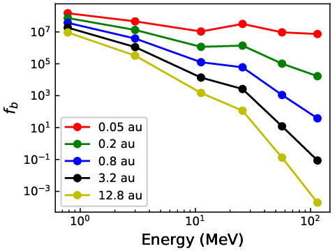
Figure 3 shows the values of distribution function at different heliocentric distances along the shock nose direction calculated by using the fitted shock parameters. It is shown that the values of distribution function can be represented by the power-law shape or the power-law shape with an exponential tail, which is consistent with the result of shock acceleration studies (Ellison & Ramaty 1985; Giacalone & Kóta 2006; Zuo et al. 2011; Kong et al. 2019, e.g.,).
IV.2 Results
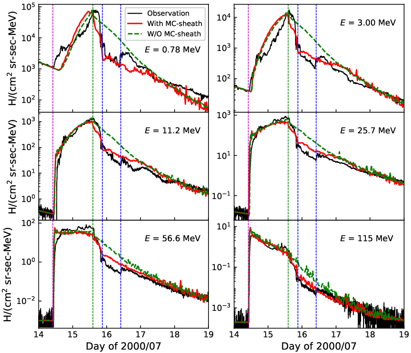
The simulation results are presented in Figure 4 where the black solid curves are the observations while the red solid curves represent the simulation results obtained by incorporating the MC and sheath into the SPTC. The pink vertical line denotes the flare onset, before which the observed proton intensities are used to obtain the backgrounds that are added to the simulated fluxes. The green vertical line represent the shock arrival while the blue vertical lines show the arrival and departure times of MC. It is shown that the simulations can fit the observations well, and the two-step decrease is reproduced between the arrivals of shock and MC’s leading edge.
To evaluate the effect of sheath-MC structure on SEPs, the simulation results without MC and sheath are also presented in Figures 4 by the green dashed curves. It is shown that the shape of the green dashed curves is the general one exhibited in the literature (Wang et al. 2012; Qin & Qi 2020, e.g.,) without rapid decline phase after the shock passage of the Earth. The comparison between the green dashed and red solid curves shows the effect that the sheath-MC structure can reduce SEP intensities when it arrived at the Earth, which lasted about 2 days. The comparison also indicates that the sheath-MC structure hardly affected the SEP intensities before it reached the Earth.
To further explore the respective influences of MC and sheath on SEPs, the simulation results for 11.2 MeV protons with only MC or sheath are presented in Figure 5(a) by the blue or orange curves, respectively. All the other lines in Figure 5(a) are the same as that in Figure 4. Figure 5(b) presents the difference between the four curves and the green curve in Figure 5(a). The simulation result with only MC, i.e., the blue curve is lower and higher than the green curve before and after the MC arrival, respectively. It is also shown that, the simulation result with only sheath, i.e., the orange curve is higher and lower than the green curve before and after the shock arrival, respectively, which is similar to the “diffusion barrier” effect (Luo et al. 2017; Luo et al. 2018, e.g.,). The simulation result with sheath-MC, i.e., the red curve is almost always lower than the green curve, and the first decrease is deeper than the second decrease. The event-integrated fluences of the blue, orange, and red curves are 4%, 23%, and 27% less than that of the green curve, respectively. Therefore, the sheath plays an important role in the decrease of SEP intensities, while the MC contributes to the formation of the second step decrease.
It is also necessary to investigate the respective impacts of local background magnetic field and turbulence level on SEPs. Next, in our study we include the sheath-MC structure. The simulation results with turbulence levels set according to Section IV.1 with the local background magnetic fields the same as that of ambient solar wind are plotted in Figure 5(c) by the blue curve. The simulation results with only the local background magnetic fields different from that of ambient solar wind is presented by the orange curve in Figure 5(c). The other lines are the same as that in Figure 5(a). Figure 5(d) has the same format as Figure 5(b) except that it is originated from Figure 5(c). It is clear that neither the blue curve nor the orange curve can produce the two-step decrease. We can show that the event-integrated fluences of the blue, orange, and red curves are 1%, 16%, and 27% less than that of the green curve, respectively, which indicates that the combination of turbulence and the enhancement of local background magnetic field can produce stronger effect in the decrease of SEP intensities.
V CONCLUSIONS AND DISCUSSION
In this work, we investigate the proton intensity-time profiles observed near the Earth for GLE59. It is shown that, the intensities have a rapid two-step decrease after the ICME shock arriving at the Earth for 1 to 100 MeV protons, which is clearer with higher energy. The two-step decrease is assumed to be caused by the sheath region and MC. To reproduce the phenomenon, a simplified sheath-MC structure is incorporated into the SPTC for simulating the transport of shock accelerated energetic particles.
The shock is treated as a moving source of SEPs with uniform speed, which is determined by dividing the Sun-Earth distance by the shock transit time, and the longitude and latitude of shock nose are set to the same as that of the corresponding solar flare. For simplicity, the MC and sheath are set as thick spherical caps with the direction, speed, and angular width set as the same as that of the shock. The Parker field is chosen as the local background magnetic field in solar wind, while the Parker field plus a magnetic enhancement represented by Equation (5) is adopted as the local background magnetic field in sheath-MC structure. Besides, the turbulence levels in MC and sheath are set to lower and higher than that in solar wind, respectively.
The simulation results indicate that the observed proton intensity-time profiles of GLE59 can be fitted well when a sheath-MC structure is placed behind the ICME shock for 1 to 100 MeV protons, and the two-step decrease of proton intensities is reproduced when the sheath and MC’s leading edge arrived at the Earth. Besides, the comparison between the simulation results with and without sheath-MC structure shows that the sheath-MC structure hardly affected the proton intensities before the shock arrived at the Earth, while it reduced the proton intensities after the shock arrival. The reducing effect lasted about 2 days. The first decrease is found to be deeper than the second one. Furthermore, The simulation results with only sheath or MC infers that the sheath contributed most of the decrease and the MC played an important role in the formation of the second step decrease. We also investigate that the effect of the combination of the turbulence and local background magnetic field in sheath-MC structure is greater than the simply superimposing of their respective effects on reducing SEP intensities.
The simulation results show that the sheath contributed most of the decrease and the first decrease is deeper than the second one, which can be explained by two reasons. Firstly, the magnetic focusing effect occurs if magnetic field is in-homogeneous, so that the strong focusing effects in sheath and MC due to the rapid change of the local background magnetic fields acting as magnetic mirrors to block the passage of particles, thus reducing SEP intensities. The magnetic focusing effect in sheath is greater than that in MC because the magnetic field in sheath varies faster than that in MC. Secondly, the turbulence level in sheath is higher than that in MC, resulting in shorter parallel mean free path of energetic particles in sheath than that in MC, and consequently the energetic particle intensities will be reduced (Luo et al. 2017; Luo et al. 2018, e.g.,).
It is impossible to measure the time-varying magnetic field of overall space now. For simplicity, the Parker field is chosen as the solar wind magnetic field and the Parker field plus a magnetic field enhancement is used as the magnetic field in sheath-MC structure. Furthermore, we use a simplified analytical magnetic field enhancement in sheath-MC model, which is not divergence-free, for the preliminary study of the transport of SEPs. The magnetic enhancement is set in radial direction for simplicity since it is difficult for us to provide a self-consistent analytical three-dimensional sheath-MC model, causing the modeled azimuthal and polar angles inconsistent with observations. Since the energetic particles’ diffusion process depends on the direction of local magnetic field, the inaccuracy of magnetic enhancement direction would make the simulation result different from observation. However, we think the magnetic mirror effect from this simplified model is still successful to reproduce the observational characteristics. It is assumed that we can roughly describe the general characteristics of SEPs flux affected by the sheath and MC with this model. In the future, we may adopt an analytical sheath-MC structure without divergence instead. In addition, to provide a local background magnetic field, we may use a three-dimensional magnetohydrodynamic simulation (Luo et al. 2013; Pomoell & Poedts 2018; Wijsen et al. 2019, e.g.,) with some divergence-free schemes (Balsara & Kim 2004).
In this work, the shock is treated as a moving source of energetic particles with a pre-described distribution function Equation (2). According to the fitted values of and in Table 2, the distribution function diminishes along the radial direction gradually, and the decay is faster if the energy is higher. It is reasonable because high energy particles are believed to be produced near the corona. The research on the acceleration of energetic particles (Kong et al. 2017; Kong et al. 2019; Qin et al. 2018; Kong & Qin 2020, e.g.,) by shocks can provide a more fidelity source, the including of which in this work may promote the understanding of the effects of sheath and MC.
The parallel and perpendicular diffusion is described by well established models, i.e., Equations (12) (15). However, the turbulence parameters in these equations are simplified, for example, the radial dependent is not considered. With the current progress in turbulence theory by the community (Zank et al. 2018; Zhao et al. 2018; Adhikari et al. 2020, e.g.,), we can better understand the transport of SEPs by using radial and time dependent turbulence parameters. Besides, The Parker Solar Probe (PSP) can provide near-Sun solar wind and SEP observations (Bale et al. 2019; Kasper et al. 2019; McComas et al. 2019) that can promote the understanding of the radial evolution of turbulence, ICMEs, shocks, and SEPs, which are important to our studies. Therefore, we will adopt the new achievement about the understanding of solar wind turbulence in the future research.
References
- Adhikari et al. (2020) Adhikari, L., Zank, G. P., Zhao, L.-L., et al. 2020, ApJS, 246, 38
- Bale et al. (2019) Bale, S. D., Badman, S. T., Bonnell, J. W., et al. 2019, Nature, 576, 237
- Balsara & Kim (2004) Balsara, D. S., & Kim, J. 2004, ApJ, 602, 1079
- Beeck & Wibberenz (1986) Beek, J., & Wibberenz, G. 1986, ApJ, 311, 437
- Bieber et al. (2002) Bieber, J. W., Dröge, W., Evenson, P. A., et al. 2002, ApJ, 567, 622
- Bieber et al. (1994) Bieber, J. W., Matthaeus, W. H., Smith, C. W., et al. 1994, ApJ, 420, 294
- Burlaga et al. (1981) Burlaga, L., Sittler, E., Mariani, F., et al. 1981, J. Geophys. Res., 86, 6673
- Cane (1993) Cane, H. V. 1993, J. Geophys. Res., 98, 3509
- Cane (2000) Cane, H. V. 2000, Space Sci. Rev., 93, 55
- Cane et al. (1986) Cane, H. V., McGuire, R. E., & von Rosenvinge, T. T. 1986, ApJ, 301, 448
- Cliver (2009) Cliver, E. W. 2009, in Proc. IAU Symp. 257, Universal Heliophysical Processes, ed. N. Gopalswamy & D. F. Webb (Cambridge: Cambridge Univ. Press), 401
- Diaz et al. (2011) Diaz, I., Zhang, M., Qin, G., et al. 2011, ICRC, 10, 40
- Dresing et al. (2012) Dresing, N., Gómez-Herrero, R., Klassen, A., et al. 2012, Sol. Phys., 281, 281
- Dröge (2000) Dröge, W. 2000, ApJ, 537, 1073
- Earl (1974) Earl, J. A. 1974, ApJ, 193, 231
- Ellison & Ramaty (1985) Ellison, D. C., & Ramaty, R. 1985, ApJ, 298, 400
- Giacalone & Kóta (2006) Giacalone, J., & Kóta, J. 2006, Space Sci. Rev., 124, 277
- Gold et al. (1998) Gold, R. E., Krimigis, S. M., Hawkins, S. E. III, et al. 1998, Space Sci. Rev., 86, 541
- Gopalswamy (2016) Gopalswamy, N. 2016, GSL, 3, 8
- Gopalswamy et al. (2012) Gopalswamy, N., Xie, H., Yashiro, S., et al. 2012, Space Sci. Rev., 171, 23
- Hasselmann & Wibberenz (1968) Hasselmann, K., & Wibberenz, G. 1968, ZGeo, 34, 353
- Hu et al. (2018) Hu, J., Li, G., Fu, S., et al. 2018, ApJ, 854, L19
- Hunana & Zank (2010) Hunana, P., & Zank, G. P. 2010, ApJ, 718, 148
- Jokipii (1966) Jokippi, J. R. 1966, ApJ, 146, 480
- Jordan et al. (2011) Jordan, A. P., Spence, H. E., Blake, J. B., et al. 2011, J. Geophys. Res., 116, A11103
- Kallenrode & Wibberenz (1997) Kallenrode, M.-B., & Wibberenz, G. 1997, J. Geophys. Res., 102, A10, 22311
- Kasper et al. (2019) Kasper, J. C., Bale, S. D., Belcher, J. W., et al. 2019, Nature, 576, 228
- Kong & Qin (2020) Kong, F.-J., & Qin, G. 2020, ApJ, 896, 20
- Kong et al. (2019) Kong, F.-J., Qin, G., Wu, S.-S., et al. 2019, ApJ, 877, 97
- Kong et al. (2017) Kong, F.-J., Qin, G., & Zhang, L.-H. 2017, ApJ, 845, 43
- Lanzerotti (2017) Lanzerotti, L. J. 2017, Space Sci. Rev., 212, 1253
- Lepping et al. (1995) Lepping, R. P., Acũna, M. H., Burlaga, L. F., et al. 1995, Space Sci. Rev., 71, 207
- Lepping et al. (2001) Lepping, R. P., Berdichevsky, D. B., & Burlaga, L. F., et al. 2001, Sol. Phys., 204, 287
- Luhmann et al. (2020) Luhmann, J. G., Gopalswamy, N., Jian, L. K., et al. 2020, Sol. Phys., 295, 61
- Luo et al. (2017) Luo, X., Potgieter, M. S., Zhang, M., et al. 2017, ApJ, 839, 53
- Luo et al. (2018) Luo, X., Potgieter, M. S., Zhang, M., et al. 2018, ApJ, 860, 160
- Luo et al. (2013) Luo, X., Zhang, M., Rassoul, H. K., et al. 2013, ApJ, 764, 85
- McComas et al. (2019) McComas, D. J., Christian, E. R., Cohen, C. M. S., et al. 2019, Nature, 576, 223
- Matthaeus et al. (1990) Matthaeus, W. H., Goldstein, M. L., & Roberts, D. A. 1990, J. Geophys. Res., 95, 20673
- Matthaeus et al. (2003) Matthaeus, W. H., Qin, G., Bieber, J. W., et al. 2003, ApJ, 590, L53
- Mazur et al. (2000) Mazur, J. E., Mason, G. M., Dwyer, J. R., et al. 2000, ApJ, 532, L79
- Mertens & Slaba (2019) Mertens, C. J., & Slaba, T. C. 2019, SpWea, 17, 1650
- Mertens et al. (2018) Mertens, C. J., Slaba, T. C., & Hu, S. 2018, SpWea, 16, 1291
- Miroshnichenko (2018) Miroshnichenko, L. I. 2018, JSWSC, 8, A52
- Onsager et al. (1996) Onsager, T. G., Grubb, R., Kunches, J., et al. 1996, Proc. SPIE, 2812, 281
- Petrovay (2010) Petrovay, K. 2010, LRSP, 7, 6
- Pomoell & Poedts (2018) Pomoell, J., & Poedts, S. 2018, JSWSC, 8, A35
- Qi et al. (2017) Qi, S.-Y., Qin, G., & Wang, Y. 2017, RAA, 17, 33
- Qin et al. (2018) Qin, G., Kong, F.-J., & Zhang, L.-H. 2018, ApJ, 860, 3
- Qin & Qi (2020) Qin, G., & Qi, S.-Y. 2020, A&A, 637, A48
- Qin & Wang (2015) Qin, G., & Wang, Y. 2015, ApJ, 809, 177
- Qin et al. (2013) Qin, G., Wang, Y., Zhang, M., et al. 2013, ApJ, 766, 74
- Qin & Wu (2018) Qin, G., & Wu, S.-S. 2018, ApJ, 869, 48
- Qin & Wu (2020) Qin, G., & Wu, S.-S. 2020, ApJ, to be submitted
- Qin et al. (2006) Qin, G., Zhang, M., & Dwyer, J. R. 2006, J. Geophys. Res., 111, A08101
- Rao et al. (1968) Rao, U. R., McCracken, K. G., & Bukata, R. P. 1968, CaJPh, 46, S844
- Reames et al. (1997) Reames, D. V., Kahler, S. W., & Ng, C. K. 1997, ApJ, 491, 414
- Reames (1999) Reames, D. V. 1999, Space Sci. Rev., 90, 413
- Reames (2017) Reames, D. V. 2017, Solar Energetic Particles (Berlin: Springer)
- Reames (2020) Reames, D. V. 2020, Space Sci. Rev., 216, 20
- Richardson & Cane (2010) Richardson, I. G., & Cane, H. V. 2010, Sol. Phys., 264, 189
- Richardson & Cane (2011) Richardson, I. G., & Cane, H. V. 2011, Sol. Phys., 270, 609
- Schlicheiser (2002) Schlicheiser, R. 2002, Cosmic Ray Astrophysics (Berlin: Springer)
- Shalchi et al. (2004) Shalchi, A., Bieber, J. W., Matthaeus, W. H., et al. 2004, ApJ, 616, 617
- Shalchi et al. (2010) Shalchi, A., Li, G., & Zank, G. P. 2010, Ap&SS, 325, 99
- Skilling (1971) Skilling, J. 1971, ApJ, 170, 265
- Tan (2017) Tan, L. C. 2017, ApJ, 846, 18
- Tan et al. (2009) Tan, L. C., Reames, D. V., Ng, C. K., et al. 2009, ApJ, 701, 1753
- Teufel & Schlickeiser (2003) Teufel, A., & Schlickeiser, R. 2003, A&A, 397, 15
- van Driel-Gesztelyi & Culhane (2009) van Driel-Gesztelyi, L., & Culhane, J. L. 2009, Space Sci. Rev., 144, 351
- Wang & Qin (2015) Wang, Y., & Qin, G. 2015, ApJ, 806, 252
- Wang et al. (2012) Wang, Y., Qin, G., & Zhang, M. 2012, ApJ, 752, 37
- Wang et al. (2014) Wang, Y., Qin, G., Zhang, M., et al. 2014, ApJ, 789, 157
- Weygand et al. (2009) Weygand, J. M., Matthaeus, W. H., Dasso, S., et al. 2009, J. Geophys. Res., 114, A07213
- Weygand et al. (2011) Weygand, J. M., Matthaeus, W. H., Dasso, S., et al. 2011, J. Geophys. Res., 116, A08102
- Wijsen et al. (2019) Wijsen, N., Aran, A., Pomoell, J., et al. 2019, A&A, 622, A28
- Wu & Qin (2018) Wu, S.-S., & Qin, G. 2018, J. Geophys. Res.: Space Physics, 123, 76
- Yu et al. (2010) Yu, X. X., Lu, H., Le, G. M., et al. 2010, Sol. Phys., 263, 223
- Zank et al. (2018) Zank, G. P., Adhikari, L., Zhao, L.-L., et al. 2018, ApJ, 869, 23
- Zank & Matthaeus (1992) Zank, G. P., & Matthaeus, W. H. 1992, J. Geophys. Res., 97, 17189
- Zank & Matthaeus (1993) Zank, G. P., & Matthaeus, W. H. 1993, PhFlA, 5, 257
- Zhang & Burlaga (1988) Zhang, G., & Burlaga, L. F. 1988, J. Geophys. Res., 93, 2511
- Zhang (1999) Zhang, M. 1999, ApJ, 513, 409
- Zhang et al. (2009) Zhang, M., Qin, G., & Rassoul, H. 2009, ApJ, 692, 109
- Zhao et al. (2018) Zhao, L.-L., Adhikari, L., Zank, G. P., et al. 2018, ApJ, 856, 94
- Zuo et al. (2011) Zuo, P., Zhang, M., Gamayunov, K., et al. 2011, ApJ, 738, 168


(d) A sectional view of the IMF (black spiral curves), shock (red arc), sheath (yellow area), and MC (green area) through the ecliptic plane.

| ColoraaIt denotes the color of the colored solid curves in Figure 2(a). | ||||
|---|---|---|---|---|
| Green | 10 | 0.42 | 0.05 | 5 |
| Pink | 10 | 0.26 | 0.09 | 5 |
| Orange | 4 | 0.21 | 0.1 | 5 |
| Blue | 24 | 0.03 | 0.56 | 5 |
| Red | 9 | -0.29 | 0.3 | 5 |
| Type | Parameter | Meaning | Value |
|---|---|---|---|
| Shock | half angular width | ||
| speed | 1406 km/s | ||
| attenuation constant in radial | 0.5 | ||
| power-law index of | 0.86 | ||
| attenuation constant in angular | 10∘ | ||
| power-law index of | 0 | ||
| Solar wind | speed | 450 km/s | |
| radial strength of IMF at 1 au | 3.62 nT | ||
| total strength of IMF at 1 au | 5 nT | ||
| MC | half thickness | 0.22 au | |
| distance between MC center and shock | 0.45 au | ||
| Sheath | half thickness | 0.08 au | |
| Others | angular speed of solar rotation | 2/25.4 rad/day | |
| inner boundary of simulation | 0.05 au | ||
| outer boundary of simulation | 50 au |
| Parameter | Meaning | Value |
|---|---|---|
| turbulence level in solar wind | 0.3 | |
| turbulence level in sheath | 1.6 | |
| turbulence level in MC | 0.1 | |
| slab correlation length | 0.025 au | |
| 2D correlation length | 0.0096 au | |
| Kolmogorov spectral index | ||
| non-linear effect index |