An Overview of Deep Learning Architectures in Few-Shot Learning Domain

Most commonly used data-sets for few shots learning are Mini-ImageNet, and Omniglot data-set. Omniglot is a data-set is specially designed to compare and contrast the learning abilities of humans and machines. The data-set contains handwritten characters of 50 languages (alphabets) with 1623 total characters. The data-set is divided into a background set and an evaluation set. Background set contains 30 alphabets (964 characters) and only this set should be used to perform all learning (e.g. hyper-parameter inference or feature learning). The remaining 20 alphabets are for pure evaluation purposes only. Each character is a 105 x 105 greyscale image. There are only 20 samples for each character, each drawn by a distinct individual(Refer Figure 2).
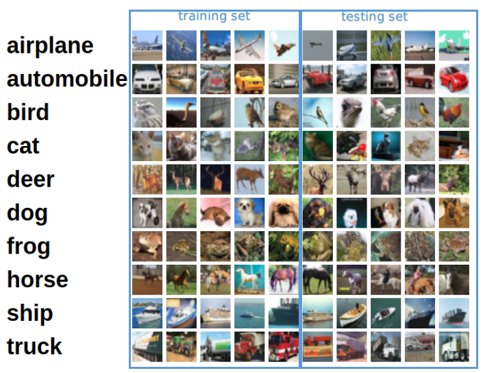
Mini-Imagenet as the name suggests if the small version of Image-Net data-set, specifically designed for Few-Shots Learning Image Classification Task, Refer Figure 1.

A Siamese network[4], as the name suggests, is an architecture with two parallel layers. In this architecture, instead of a model learning to classify its inputs using classification loss functions, the model learns to differentiate between two given inputs. It compares two inputs based on a similarity metric, and checks whether they are same or not. This network consists of two identical neural networks, which share similar parameters, each head taking one input data point (see fig. 2). In the middle layer, we extract similar kinds of features, as weights and biases are the same. The last layers of these networks are fed to a loss function layer, which calculates the similarity between the two inputs. The whole idea of using Siamese architecture[5] [1] is not to classify between classes but to learn to discriminate between inputs. So, it needed a differentiating form of loss function such as the contrastive loss function.

Matching networks [7], in general, proposes a framework which learns a network that maps a small data-set and an unlabeled example to its label. When it comes to a small data-set, we come across the problem of over-fitting and under-fitting which can be alleviated using regularization and data augmentation respectively; but still, it doesn’t solve the root cause of the issue. The other problem is that learning of parameters is very slow, requiring various weight updates using stochastic gradient descent; whereas many non-parametric models, such as k-nearest neighbor, doesn’t even require any form of training; it stores data-set and makes a decision based on a metric. Matching networks incorporate the best characteristic of both parametric and non-parametric models, also famously known as Differential Nearest neighbor. Matching networks are designed to be two-fold:

1. 1.

   Modeling level: At Modeling level, they proposed Matching nets, which uses advances made in attention and memory that enable fast and efficient learning.

2. 2.

   Training procedure: At Training Level, they have one condition that distribution of training and test set must be same. For example: show a few examples per class, switching the task from mini-batch to mini-batch, similar to how it will be tested when presented with a few examples of a new task.

In simpler terms, matching networks learn the proper embeddings representation and use cosine similarity measure to ensure whether a test data point is something ever seen or not.

Matching Networks is a neural network model that implements an end-to-end training procedure that combines feature extraction and differentiable k-NN with cosine similarity. Matching network’s architecture is majorly inspired by the attention model and memory-based networks. In all these models, a neural attention mechanism is defined to access a memory matrix, which stores useful information to solve the task at hand. To begin with, first we need to understand certain terminologies of Matching Network:

1. 1.

   Label Set: This is the sample set of all possible categories. For example, if we have 1,000 categories and as part of sampling from the database we only use only 5 categories.

2. 2.

   Support Set: This is the sampled input data points (for example, images) of label set categories.

3. 3.

   Batch: Similar to support set, batch is also a sampled set consisting of input data points of Label Set Categories.

4. 4.

   N-way K-Shot Method: Here, N is the size of the support set. In simpler terms, the number of possible categories in the training set. For example, in the figure that follows, we have four different types of dog breeds, and we are planning to do 5-shot learning method, that is, have at least five examples of each category. This will make Matching Network Architecture as 4 way 5 shot learning.

The key idea of Matching networks is to map images to an embeddings space, which also encapsulates the label distribution and then project test image in the same embedding space using different architecture; later, use cosine similarity to measure the similarity metric.

The early development stages of the field of Artificial Intelligence was heavily dominated with the symbolic approach - which attempted to explain how information processing systems like human brain might work in terms of symbols, structures and rules to manipulate those symbols and structures. It wasn’t until about 1980s when the field of AI took a different approach - connectionism, neural networks being the most promising modeling technique of connectionism. The advent of neural networks met with two heavy criticisms. First neural networks typically accept fixed sized inputs and won’t be much useful as most of the input in real life problems is variable length (sequence of frames in video, text, speech). Second, neural networks seem unable to bind values to specific locations within data structures which is heavily employed by two information systems we know of - human brain and computers. The first criticism about variable length input was answered by Recurrent Neural Networks (RNNs) which have achieved state-of-the-art performance on many tasks. Neural Turing Machines [9], the topic of discussion in this section tries to answer second criticism by giving external memory to neural networks and a method to learn to use it. We will discuss the overall architecture of Neural Turing Machine (NTM) in this section which is foundational to understanding Memory-Augmented Neural Networks (MANN) [10] which modifies NMT architecture and adapt it for few-shot learning task.

Modern computers have advanced a lot over past 50 years but they are still composed of three systems - memory, control flow and arithmetic/logic operations. There’s also biological evidence that working memory is crucial in quick and meaningful store and retrieval of information. The same is also established extensively by the computational neuroscience field. Taking inspirations from this, A NTM [9] is fundamentally composed of a neural network - controller and a 2D matrix called the memory bank (or memory matrix). At each time step, the neural network receives some input and generates some output corresponding to that input. In the process of doing so, it also accesses the internal memory bank and performs read and/or write operations on it. Drawing inspiration from traditional turing machines, NMT uses the term ’head’ to specify the memory location(s). The overall architecture is shown in Figure 4. There’s one challenge in this architecture, If we access the memory location by specifying row and column index in the memory matrix, we can’t take gradient of that index. This operation is not back-propagable and would restrict the training of NMT using standard back-propagation and gradient descent based optimization techniques. To circumvent this problem, the controller of the NTM [11] interacts with memory using ’blurry’ read and write operations that interacts with all elements of the memory to varying degrees. More precisely the controller produces weights over all memory locations in a differentiable manner which helps in training the network end-to-end using standard gradient based optimization methods.

1. 1.

   Modeling: The memory matrix at time step $t(M_{t})$ has $R$ rows and $C$ columns. There’s an attention mechanism which dictates where the head should read/write from. This attention vector, generated by controller is a length- $R$ vector called weight vector $W_{t}$ where each entry of this vector $W_{t}(i)$ is the weight for the $i^{th}$ row of the memory bank. The weight vector is normalized which means it satisfies following conditions:

   $0\leq w_{t}(i)\leq 1$ and , $\sum_{i=1}{R}w_{t}(i)=1$

2. 2.

   Reading: The read head will return a length- $C$ vector $r_{t}$ that is a linear combination of the memory’s rows $M_{t}(i)$ scaled by the weight vector:

   $r_{t}\leftarrow\sum_{i=1}{R}(w_{t}(i)M_{t}(i))$

3. 3.

   Writing: Writing is a combination of two steps: erasing and adding. In order to erase old data the write head uses an additional length- $C$ erase vector, $e_{t}$ along with the weight vector. The following equations defines the intermediate step of erasing the rows.

   $M_{t}^{erased}(i)\leftarrow M_{t-1}(i)[1-w_{t}(i)e_{t})$ Finally, the write head uses length- $C$ add vector $a_{t}$ along with $M^{erased}$ from above and weight vector to update the rows of the memory matrix. $M_{t}(i)\leftarrow M_{t}^{erased}+w_{t}(i)a_{t}$

4. 4.

   Addressing: The key to read and write operation is the weight vector which indicates which rows to read/write from/to. The controller produces this weight vector in four stages. Each stage produces in an intermediate vector which gets passed to the next stage. The first stage is content-based addressing, the goal of which is to generate a weight vector based on how similar each row is to some key vector $k_{t}$ of length $C$. More precisely, controller emits vector $k_{t}$ which is compared to each row of $M_{t}$ using cosine similarity measure, defined below

   $K(u,v)=\frac{u.v}{||u||.||v||}$

   The content weight vector is not normalized yet, so its normalized with the following operation.

   $w_{t}^{c}(i)=\frac{exp(\beta_{t}K(k_{t},M_{t}(i)))}{\sum_{j}\exp(\beta_{t}K(k_{t},M_{t}(j)))}$

   The next stage is the location based addressing which focuses on read/write from specific memory locations as opposed to read/write specific location values done by stage 1. In the second stage, a scalar parameter $g_{t}\in(0,1)$ called the interpolation gate, blends the content weight vector $w_{t}^{c}$ with the previous time step’s weight vector $w_{t-1}$ to produce the gated weighting $w_{t}^{g}$ . This allows the system learn when to use (or ignore) content-based addressing.

   $w_{t}^{g}\leftarrow g_{t}w_{t}^{c}+(1-g_{t})w_{t-1}$

   In the third stage, after interpolation, the head emits a normalized shift weighting $s_{t}$ to perform shift modulo $R$ operation (i.e. move rows upwards or downwards). This is defined by the operation below.

   $\tilde{w_{t}}(i)\leftarrow\sum_{j=0}^{R-1}w_{t}^{g}(j)s_{t}(i-j)$

   The fourth and final stage, sharpening, is used to prevent the shifted weight $\tilde{w_{t}}$ from blurring. This is done with a scalar $\gamma\geq 1$ and applying the operation.

   $w_{t}(i)\leftarrow\frac{\tilde{w_{t}}(i)^{\gamma_{t}}}{\sum_{j}\tilde{w_{t}}(j)^{\gamma_{t}}}$

All the operations, including read, write and four stages of addressing are differentiable and thus the entire NMT model could be trained end-to-end with back-propagation and any gradient descent based optimizer. The controller is a neural network which could be a feed-forward network or even a recurrent neural network like LSTMs. Now that we understand the architecture and the working of NTM, we can dive into Memory Augmented Neural Networks which is a modification of NMT and has been modified to excel at few-shot learning.

The goal of Memory Augmented Neural Network (MANN) [10] is to excel at few-shot learning task. The NMT controller, as we read earlier uses both content-based addressing and location-based addressing. On the other hand, the MANN controller uses only content-based addressing. There are two reasons to do this. One reason is that location-based addressing is not required for the few-shot learning task. In this task, for a given input, there are only two actions a controller might need to take and both actions are content dependent and not location dependent. One action is that the input is very similar to previously seen input in which case we might what to update whatever is there in memory. The other action is that current input is not similar to previously seen inputs in which case we don’t want to overwrite the recent information but the least used memory location. The memory module, in this case, is called Least Recently Used Access (LRUA) module.

1. 1.

   Reading: The read operation of MANN is very similar to the read operation of NTMs, with a minor difference that the weight vector here uses only content bases addressing (stage -1 of NMT addressing). More precisely, the controller uses normalized read weight vector, $w_{t}^{r}$ is used along with the rows of the $M_{t}$ to produce read vector $r_{t}$. $r_{t}\leftarrow\sum_{i}^{R}(w_{t}^{r}(i)M_{t}(i)$ The read-weight vector $w_{t}^{r}$ is produced by controller defined by the operations below. $w_{t}^{r}=\frac{exp(K(k_{t},M_{t}(i))}{\sum_{j}exp((k_{t},M_{t}(j)))}$ where, operation $K()$ is the cosine similarity , similar to the one defined for NMTs above.

2. 2.

   Writing: To write to the memory, the controller interpolates between writing to the most recently read memory rows and writing to least recently read memory rows. $w_{t}^{w}\leftarrow\sigma(\alpha)w_{t-1}^{r}+(1-\sigma(\alpha))w_{t-1}^{lu}$ $M_{t}(i)\leftarrow M_{t-1}(i)+w_{t}^{w}(i)k_{t}$ $w_{t}^{u}\leftarrow\gamma w_{t-1}^{u}+w_{t}^{r}+w_{t}^{w}$

Meta Networks [12] as the name suggests is a form of Model-based Meta-Learning Approach. Similar to how Meta-Learning approaches, In meta-networks also, we have a base learner and meta-learner sharing parameters where a meta-learner extracts common features of all tasks and a base learner learns the targeted task. As we can see in figure 7, Meta Networks is also equipped with external memory, similar to architecture we just read above Memory Augmented Neural Networks. The underlying key idea of Meta Networks is to learn weights in a fast manner for rapid generalizations, and it has been done by processing higher order meta information. In the next section, we will go through an understanding of architecture, extraction of meta information, and it’s parameter optimization algorithm.

Note: Previous work on Meta-learning has formulated the problem as two-level learning: slow learning of a meta-level model performing across tasks and rapid learning of a base-level model acting within each task. The goal of a meta-level learner is to acquire a general knowledge of different tasks. The knowledge can then be transferred to the base-level learner to provide generalization in the context of a single task. The base and meta-level models can be framed in a single learner.

In usual Deep Learning Methods, weights of neural networks are updated by stochastic gradient descent and many times it takes a lot of time to train, in other words, slow weights update. In Meta Networks, one solution has been suggested to improve upon this method: To utilize one neural network in parallel to original neural network, to predict the parameters of another neural network and the generated weights are called fast weights.

In MetaNet [12], loss gradients are used as meta information to enable models that learn fast weights. Slow and fast weights are combined to make predictions in neural networks just as shown in the figure above. Here, $sum$ means element-wise sum. Meta Networks Learning occurs at two levels in separate spaces: meta space and task space. here, the base learner learns in task-specific space, whereas the meta-learner learns meta-knowledge across different tasks. After training of Meta learner, the base learner first analyzes the input task and then provides the meta-learner with feedback in the form of higher order meta information(gradients) to explain its own status in the current task space.

There are two important components of a MetaNet as shown in figure 6:

1. 1.

   Embedding function $(f_{\theta})$: As part of Meta Net, we train Embedding generator function, which is then used to compare features of two different data points, very similar to what we have in Siamese Networks.

2. 2.

   Base Learner Model $g_{\phi}$: It is parameterized by weights, and completes the actual learning task.

As we have two different types of networks trained in parallel: fast, and slow network, therefore we also need to get Embedding Function and a Base Learner Model for a fast network:

1. 1.

   Embedding Function$(F_{w})$: an LSTM architecture, for learning fast weights $\theta$ of the embedding function$(f_{\theta})$ of slow network.

2. 2.

   Base Learner Model $(G_{v})$: a neural network parameterized by v learning fast weights $\phi$ for the base learner $g_{\phi}$from its loss gradients.

For training, Meta Networks also follow a similar training procedure as of Matching Networks. Here, also we obtain training data contains multiple pairs of datasets: support set S = $(x_{i}^{\prime},y_{i}^{\prime})$ and training set U= $(x_{i},y_{i})$ . So, now we have four networks and four sets of model parameters to learn, $(\theta,\phi,w,v)$. [12] also proposed the meta learning based algorithm to train networks as shown in figure 7

The goal of Model Agnostic Meta-Learning [13] architecture is to quickly learn a new task from a small amount of new data. The key idea of this approach is to train the models’ initial parameters using a different data-set, such that as the new task comes, the model gives maximum performance by using already initialized parameters, to fine-tune the architecture through one or more gradient steps. As we know that Neural Networks use Gradient descent algorithm to train, so the method of training a model’s parameters such that a few gradient steps can optimize loss function, and give good results, can be viewed from a feature learning standpoint as building an internal representation. As it is very generic, therefore can be used for various tasks. The primary contribution of this work is a simple model and task-agnostic algorithm that trains a model’s parameters such that a small number of gradient updates will lead to fast learning on the new task. The Objective of Model-Agnostic Meta-Learning (MAML) [13] is to provide a good initialization of a model’s parameters to achieve optimal fast learning on a new task with less number of gradient steps. It also attempts to avoid overfitting scenarios, which happens while training a Neural Network with less amount of data architecture.

As we can see in the figure 8 parameters $\theta$ are close to all the 3 optimal parameters of task 1, 2, and 3 which makes $\theta$ the best parameters initialization that can quickly adapt to different new tasks. As a result, only a small change in the parameters $\theta$ will lead to an optimal minimization of the loss function of any task. This is the key idea of MAML, that somehow we learn $\theta$ through the original dataset, so while fine-tuning on the real dataset, we just have to move a small step. For One/Few Shots Learning, first, we prepare our data. For a particular task say, $T_{i}$ we have data samples which are forming task distribution of form $P(T)$ (Probabilistic distribution across all tasks). Our aim is to train a model to learn task $T_{i}$ from K data points and feedback generated by Loss , $L(T_{i})$. During meta-training, a task $T_{i}$ is sampled from $P(T)$ i.e; training data available, then model is trained with K samples and feedback from the corresponding loss $L(T_{i})$ from $T_{i}$ , and then tested on new samples from $T_{i}$ . The model is then improved by considering how the test error on new data changes with respect to the parameters. In effect, the test error on sampled tasks $T_{i}$ serves as the training error of the meta-learning process. At the end of the training, new tasks are sampled from $p(T)$, and meta-performance is measured by the model’s performance after learning from K samples.

$L_{T_{i}}(f_{\phi})=\sum_{x^{j},y^{j}\backsim T_{i}}||f_{\phi}(x^{(j)})-y^{(j)}||_{2}^{2}$

where $x^{(j)},y^{(j)}$ are sampled from task $T_{i}$. To learn more in detail about steps followed in maml optimization Algorithms, please take a look at the algorithm published in the paper [13].

As the name suggests, LSTM meta-learner [14] algorithm is specifically designed on LSTM Architecture because a cell-state update in LSTM is similar to gradient-based update in backpropagation, and information about the history of gradients help in optimizing model better. This Optimization Algorithm is trained to optimize a learner neural network classifier. It captures the knowledge of both the short term of a particular task and common long term.

LSTM meta learner is heavily inspired from connection in logic of Gradient descent and LSTM cell update. Ravi et al., [14] explained that iff we look into update method of Gradient Descent, we will see an equation like this:

$\theta_{t}=\theta_{t-1}-\alpha_{t}\bigtriangledown L_{t}$

here, $\theta_{t}$ is parameters at t time step, $\bigtriangledown L_{t}$ is gradient of Loss at t, and $\alpha_{t}$ is learning rate at time t.

One observation that authors of LSTM meta learner made was, that this update looks very similar to how cells get updated in LSTMs.. So, The Key idea of Meta-Learner LSTM is to learn an update rule for training a neural network. Lets first dive in how a cell state is defined in an LSTM.

$c_{t}=f_{t}\odot c_{t-1}+i_{t}\odot\bar{c_{t}}$

If we put $f_{t}=1,c_{t-1}=\theta_{t-1},i_{t}=\alpha_{t}$ and $\bar{c_{t}}=\bigtriangledown L_{t}$ , we will get a gradient descent update rule. Considering this, Logically, we want to learn $i_{t}$, as that is essentially similar to estimating the learning rate of gradient descent. so, LSTM Meta Learner define $i_{t}$ as:

$i_{t}=\sigma(W_{I}.[\bigtriangledown L_{t},L_{t},\theta_{t-1},i_{t-1}]+b_{I})$

i.e; a sigmoid function with a combination of current gradient, Loss, and previous learning rate $i_{t-1}$.

For $f_{t}$, it should be 1, but to avoid problems of shrinking gradients, and exploding gradients. It has been chosen as:

$f_{t}=\sigma(W_{F}.[\bigtriangledown L_{t},L_{t},\theta_{t-1},f_{t-1}]+b_{F})$

i.e; sigmoid function with a combination of current gradient, Loss, and forget gate.

Semi-supervised learning[15] is a machine learning technique that involves training a model on both labeled and unlabeled data. In traditional supervised learning, models are trained only on labeled data, which is expensive and time-consuming to obtain. However, with semi-supervised learning, models can leverage the vast amount of unlabeled data available to improve performance on labeled data.

Suppose we have 10,000 data points, out of which only 20,000 are labeled, and the rest 80,000 are unlabeled. In such cases, we can take the help of semi-supervised learning to train a more accurate model. Semi-supervised learning [15] goes through a pseudo-labeling technique to increase the training set. In this technique, we train a model using the 20,000 labeled dataset and use it on an equally sized test dataset to create pseudo-labels for the unlabeled data points. After obtaining pseudo-labels, we concatenate the real labels with the pseudo-labels and real features with the pseudo-features. We then train a new model on the concatenated dataset, which has been shown to be more accurate than the initial model. We repeat this process until optimal accuracy is achieved.

Semi-supervised learning works well in scenarios where labeled data is scarce, and there is a vast amount of unlabeled data available. By leveraging the unlabeled data, models can gain a better understanding of the population structure in general, leading to improved performance on the labeled data. Semi-supervised learning has been applied in various fields such as computer vision, natural language processing, and speech recognition.

However, it is important to note that semi-supervised learning is not a panacea, and it may not always lead to improved performance. The success of semi-supervised learning depends on various factors such as the quality of the unlabeled data, the complexity of the task, and the type of model used. Additionally, the pseudo-labeling technique may introduce errors if the model makes incorrect predictions on the unlabeled data. Therefore, it is crucial to validate the accuracy of the pseudo-labels before using them to train the model.

In Imbalanced Learning [16] scenario, we have an imbalanced data-set i.e; we have more samples from one class, whereas very few examples of other categories, this is also popularly known as skewed distribution data-set. Let’s take a look at some popular methods for dealing with a skewed data-set.

1. 1.

   Choice of Metric: There are various forms of metrics[17] that can help in assessing the accuracy of a model, such as Confusion Matrix, Precision, Recall, and F1-Score.

2. 2.

   Choice of Machine Learning Algorithm: Parametric Algorithms learn their parameters through the data-set, so if the data-set is biased, it is most likely that the parametric model will also be biased. Non-parametric approaches such as K-Nearest Neighbor, Decision Trees etc. Ensembles such as Random Forest, Adaboost, XG-Boost are proven to be the best approaches when it comes to a biased data-set.

3. 3.

   Choice of Data Sampling Methods: Data Sampling can also be considered to ensure that data-set doesn’t remain skewed.

This is close to few-shot Learning, as the machine learning model we are expected to create should be able to learn distribution from a few examples.

Transfer Learning [18] is a machine learning technique that involves the application of knowledge gained from one task to another related task. It is based on the idea that the knowledge acquired by a model while solving one task can be leveraged to help improve the performance of a different task.

The primary motivation behind transfer learning is to reduce the need for large amounts of labeled data for a new task. In many real-world scenarios, it is expensive and time-consuming to collect large amounts of labeled data. However, with transfer learning, the knowledge gained from solving a related task can be used to train a model on the new task, reducing the amount of labeled data required.

There are three main types of transfer learning:

1. 1.

   Inductive Transfer Learning: In this approach, the model is first trained on a large, diverse dataset and then fine-tuned on the new task. The idea behind this approach is that the model has already learned features that are relevant to the new task, and fine-tuning helps to refine those features.

2. 2.

   Transductive Transfer Learning: This approach involves transferring knowledge between related tasks, where the goal is to learn the mapping between two different domains. For example, mapping between two different languages, or between image and text domains.

3. 3.

   Unsupervised Transfer Learning: This approach involves using the knowledge gained from unsupervised learning to improve the performance of a supervised learning task. In unsupervised learning, the model learns to represent data in a way that captures its underlying structure. This representation can then be used to improve the performance of a supervised learning task that uses the same data.

Transfer learning has been applied in various fields such as computer vision, natural language processing, and speech recognition. For instance, in computer vision, transfer learning has been used to improve the performance of object recognition, object detection, and image classification. Similarly, in natural language processing[19], transfer learning has been used to improve the performance of tasks such as sentiment analysis, named entity recognition, and machine translation.

In summary, Transfer Learning is a powerful technique that enables models to leverage knowledge gained from one task to improve performance on another related task. It is particularly useful in scenarios where labeled data is scarce, and it has been applied in various fields to improve the performance of machine learning models.

References

- [1] S. Jadon and A. Garg, Hands-On One-shot Learning with Python. Packt Publishing, 2020.
- [2] S. Jadon, O. P. Leary, I. Pan, T. J. Harder, D. W. Wright, L. H. Merck, and D. L. Merck, “A comparative study of 2d image segmentation algorithms for traumatic brain lesions using ct data from the protectiii multicenter clinical trial,” in Medical Imaging 2020: Imaging Informatics for Healthcare, Research, and Applications, vol. 11318, p. 113180Q, International Society for Optics and Photonics, 2020.
- [3] S. Jadon, “Introduction to different activation functions for deep learning,” Mar 2018.
- [4] G. Koch, R. Zemel, and R. Salakhutdinov, “Siamese neural networks for one-shot image recognition,” in ICML deep learning workshop, vol. 2, 2015.
- [5] S. Jadon and A. A. Srinivasan, “Improving siamese networks for one shot learning using kernel based activation functions,” arXiv preprint arXiv:1910.09798, 2019.
- [6] C. Vargas, Q. Zhang, and E. Izquierdo, “One shot logo recognition based on siamese neural networks,” in Proceedings of the 2020 International Conference on Multimedia Retrieval, pp. 321–325, 2020.
- [7] O. Vinyals, C. Blundell, T. Lillicrap, D. Wierstra, et al., “Matching networks for one shot learning,” in Advances in neural information processing systems, pp. 3630–3638, 2016.
- [8] S. Jadon, “Ssm-net for plants disease identification in lowdata regime,” arXiv preprint arXiv:2005.13140, 2020.
- [9] A. Graves, G. Wayne, and I. Danihelka, “Neural turing machines,” arXiv preprint arXiv:1410.5401, 2014.
- [10] A. Santoro, S. Bartunov, M. Botvinick, D. Wierstra, and T. Lillicrap, “One-shot learning with memory-augmented neural networks,” arXiv preprint arXiv:1605.06065, 2016.
- [11] M. Collier and J. Beel, “Implementing neural turing machines,” in International Conference on Artificial Neural Networks, pp. 94–104, Springer, 2018.
- [12] T. Munkhdalai and H. Yu, “Meta networks,” Proceedings of machine learning research, vol. 70, p. 2554, 2017.
- [13] C. Finn, P. Abbeel, and S. Levine, “Model-agnostic meta-learning for fast adaptation of deep networks,” arXiv preprint arXiv:1703.03400, 2017.
- [14] S. Ravi and H. Larochelle, “Optimization as a model for few-shot learning,” 2016.
- [15] X. Zhu and A. B. Goldberg, “Introduction to semi-supervised learning,” Synthesis lectures on artificial intelligence and machine learning, vol. 3, no. 1, pp. 1–130, 2009.
- [16] G. Haixiang, L. Yijing, J. Shang, G. Mingyun, H. Yuanyue, and G. Bing, “Learning from class-imbalanced data: Review of methods and applications,” Expert Systems with Applications, vol. 73, pp. 220–239, 2017.
- [17] A. Jadon, A. Patil, and S. Jadon, “A comprehensive survey of regression based loss functions for time series forecasting,” arXiv preprint arXiv:2211.02989, 2022.
- [18] S. J. Pan and Q. Yang, “A survey on transfer learning,” IEEE Transactions on knowledge and data engineering, vol. 22, no. 10, pp. 1345–1359, 2009.
- [19] A. Patil and A. Jadon, “Auto-labelling of bug report using natural language processing,” arXiv preprint arXiv:2212.06334, 2022.
- [20] G. Keren, M. Schmitt, T. Kehrenberg, and B. Schuller, “Weakly supervised one-shot detection with attention siamese networks,” stat, vol. 1050, p. 12, 2018.
- [21] S. Mshir and M. Kaya, “Signature recognition using machine learning,” in 2020 8th International Symposium on Digital Forensics and Security (ISDFS), pp. 1–4, 2020.
- [22] J. Thathachar, T. Kornuta, and A. S. Ozcan, “Encoder-decoder memory-augmented neural network architectures,” Mar. 19 2020. US Patent App. 16/135,990.
- [23] M. Collier and J. Beel, “Memory-augmented neural networks for machine translation,” arXiv preprint arXiv:1909.08314, 2019.
- [24] F. Shen, S. Yan, and G. Zeng, “Meta networks for neural style transfer,” arXiv preprint arXiv:1709.04111, 2017.
- [25] Z. Chen, Y. Fu, Y.-X. Wang, L. Ma, W. Liu, and M. Hebert, “Image deformation meta-networks for one-shot learning,” in Proceedings of the IEEE Conference on Computer Vision and Pattern Recognition, pp. 8680–8689, 2019.
- [26] Z. Liu, R. Zhang, Y. Song, and M. Zhang, “When does maml work the best? an empirical study on model-agnostic meta-learning in nlp applications,” arXiv preprint arXiv:2005.11700, 2020.
- [27] H. S. Behl, A. G. Baydin, and P. H. Torr, “Alpha maml: Adaptive model-agnostic meta-learning,” arXiv preprint arXiv:1905.07435, 2019.
- [28] H. Li, D. Eigen, S. Dodge, M. Zeiler, and X. Wang, “Finding task-relevant features for few-shot learning by category traversal,” in Proceedings of the IEEE Conference on Computer Vision and Pattern Recognition, pp. 1–10, 2019.
- [29] S.-A. Rebuffi, S. Ehrhardt, K. Han, A. Vedaldi, and A. Zisserman, “Semi-supervised learning with scarce annotations,” in Proceedings of the IEEE/CVF Conference on Computer Vision and Pattern Recognition Workshops, pp. 762–763, 2020.
- [30] C. Huang, Y. Li, C. C. Loy, and X. Tang, “Learning deep representation for imbalanced classification,” in Proceedings of the IEEE conference on computer vision and pattern recognition, pp. 5375–5384, 2016.
- [31] A. Fernández, S. García, M. Galar, R. C. Prati, B. Krawczyk, and F. Herrera, Learning from imbalanced data sets. Springer, 2018.
- [32] F. Zhuang, Z. Qi, K. Duan, D. Xi, Y. Zhu, H. Zhu, H. Xiong, and Q. He, “A comprehensive survey on transfer learning,” Proceedings of the IEEE, 2020.