Comparison and Application of non-Conforming Mesh Models for Flow in Fractured Porous Media using dual Lagrange multipliers

Patrick Zulian Affiliation: Institute of Computational Science, USI Lugano, 6904 Lugano, Switzerland Email: patrick.zulian@usi.ch Philipp Schädle Affiliation: Institute of Geophysics, Department of Earth Sciences, ETH Zürich, 8092 Zürich, Switzerland. Email: philipp.schaedle@erdw.ethz.ch Liudmila Karagyaur Affiliation: Institute of Computational Science, USI Lugano, 6904 Lugano, Switzerland Email: liudmila.karagyaur@usi.ch Maria G. C. Nestola Affiliation: Institute of Computational Science, USI Lugano, 6904 Lugano, Switzerland. Affiliation: Institute of Geochemistry and Petrology, Department of Earth Sciences, ETH Zürich, 8092 Zürich, Switzerland Affiliation: nestom@usi.ch, maria.nestola@erdw.ethz.ch

Abstract

Geological settings with reservoir characteristics include fractures with different material and geometrical properties. Hence, numerical simulations in applied geophysics demands for computational frameworks which efficiently allow to integrate various fracture geometries in a porous medium matrix. This study presents a modeling approach for single-phase flow in fractured porous media and its application to different types of non-conforming mesh models. We propose a combination of the Lagrange multiplier method with variational transfer to allow for complex non-conforming geometries as well as hybrid- and equi-dimensional models and discretizations of flow through fractured porous media. The variational transfer is based on the $L^{2}$ -projection and enables an accurate and highly efficient parallel projection of fields between non-conforming meshes (e.g., between fracture and porous matrix domain).
We present the different techniques as a unified mathematical framework with a practical perspective. By means of numerical examples we discuss both, performance and applicability of the particular strategies. Comparisons of finite element simulation results to widely adopted 2D benchmark cases show good agreement and the dual Lagrange multiplier spaces show good performance. In an extension to 3D fracture networks, we first provide complementary results to a recently developed benchmark case, before we explore a complex scenario which leverages the different types of fracture meshes. Complex and highly conductive fracture networks are found more suitable in combination with embedded hybrid-dimensional fractures. However, thick and blocking fractures are better approximated by equi-dimensional embedded fractures and the equi-dimensional mortar method, respectively.

1 Introduction

Fluid flow through fractured porous media is a crucial process in the context of numerous subsurface applications, e.g. groundwater management, geothermal energy utilization, CO₂ sequestration, hazardous waste storage, and enhanced oil and gas recovery [1, 2, 3, 4, 5, 6, 7, 8]. Often, fluid flow velocities in fractures and in the porous medium matrix range over many orders of magnitudes. Therefore, single fractures and networks of fractures largely govern the characteristics of fluid transport in fracture-dominated porous media. More specifically, the detailed fracture geometry of each individual fracture has a significant influence on the fluid flow in a fracture-dominated system. While the aperture width of a fracture can vary over several orders of magnitudes, the fracture can additionally be filled with an infilling material exhibiting permeability values ranging over many orders of magnitude. As a consequence, these two aspects lead to strong differences in the transmissivity and therefore the fractures ability to permit fluid transport. Thereby, the presence and permeability of an infilling material determines if a single fracture acts as a conduit or a barrier for fluid flow [9, 10, 11, 12]. A detailed description of fluid flow through fractured porous media therefore requires comprehensive knowledge about the hydraulic properties of each individual fracture. Such properties are very difficult to obtain in the field and a detailed deterministic description of such systems is not possible [13]. Consequently, stochastic investigations are universally conducted to describe fractured media and to account for associated uncertainties [14, 9]. Due to the large number of forward simulations required by stochastic studies, highly efficient and accurate numerical methods and mesh generation approaches are needed [15, 16, 17, 18, 19].
To numerically model fractured systems, two method classes are widely used, continuum models and discrete fracture models. In the class of continuum models, fractures and porous-medium matrix are represented by separate continua within the same geometric mesh [20, 21, 22, 23]. Effective flow properties are obtained by upscaling and information between the continua needs to be transferred. In the class of discrete fracture models, fractures are represented as discrete domains in a numerical mesh [24, 25]. Here, two concepts are distinguished where the porous-medium matrix is either represented in discrete-fracture-matrix models (DFM) or neglected in discrete-fracture-networks models (DFN) [26, 9]. In classic DFMs, fracture and porous-medium matrix domains are explicitly meshed and conforming at the domain interface, i.e. conforming geometry and discretization [27, 28, 29, 30]. Due to the large complexity of fracture networks, mesh generation for such conforming DFMs can be very challenging and time consuming [31, 32, 33]. Such challenges occur in the matrix mesh domain as well as the fracture mesh domain. Due to the large length-to-width ratio of many fractures it is common to use lower-dimensional elements to represent the fracture domain, e.g. [34, 35, 36, 37]. This avoids elements with large aspect ratios in the fracture mesh and thus improves numerical performance. However, fractures with considerably large aperture width are not ideally represented by lower-dimensional elements [38]. Those fractures might be less numerous but require to generate fracture domain meshes which are equi-dimensional to the porous medium matrix domain. Further challenges are posed by the matrix mesh generation around the fractures. This is particularly difficult where fractures are close to each other or intersect with very low angles. Such configurations can lead to elements with large aspect ratios or non-physical connections, which requires fine tuning of the meshes to improve performance and stability of the solution [38]. It is important to bear in mind that this is even more challenging in 3D and makes stochastic studies with DFMs very challenging. These challenges in model generation combined with the requirements and geometrical complexities of DFMs motivated a large number of method developments and improvements, and yielding this to be an active research field.
The drawbacks associated with the classic discrete-domain approaches have triggered research on, and the development of, numerical methods that allow to use individual meshes for the fracture and porous medium matrix domains. Such methods rely on the concept of non-conforming discretizations, while the meshes might be geometrically conforming or non-conforming. Methods with non-conforming discretization but conforming geometries require the element facets of the fracture domain to align with the neighboring element facets of the porous-medium matrix domain without coinciding, e.g. mortar methods [39, 40, 41, 42, 43, 44] and discontinuos Galerking methods [45]. In contrast, fully non-conforming methods, i.e. non-conforming discretization and non-conforming geometry, require no geometrical relationship between the fracture and the porous-medium matrix domains. These methods exist for finite volume schemes, e.g. (p)EDFM [46, 47, 48, 49, 50] and for finite element schemes, e.g. extended finite element methods (XFEM) [51], or continuous Galerkin method where fractures are represented as Dirac functions [52]. XFEM approaches exist with primal formulations [53, 54, 55] and dual formulations [56, 57]. An exposition of different coupling techniques in discrete fracture networks is provided in [58], where the focus is on handling complex fracture networks without accounting the effects of the surrounding rock. Recently, Köppel et al. 2018 presented an alternative fully non-conforming finite element formulation for which Schädle et al. 2019 demonstrated its applicability in 3D. Often, non-conforming mesh methods allow for an automated mesh generation and model setup process, which enables stochastic studies with a large number of different fracture network geometries. In particular, methods that handle fracture and matrix meshes separately (i.e. non-conforming geometries), significantly reduce the work required for preparing the simulation geometries. Berre et al. 2018 provide a good overview of existing conceptual and discretization methods and discuss the differences in conforming and non-conforming methods.
The mutually non-conforming discretizations of non-conforming mesh approaches require the use of coupling techniques and information transfer between the domains. Lagrange multipliers are a common tool to couple systems of equations and they are widely used throughout various fields [62, 63]. More specifically, fictitious domain [64] and mortar [65] methods are discretization techniques based on the Lagrange multiplier [66, 67]. In the context of DFMs, Lagrange multipliers have thus far been applied for both, fully non-conforming and non-conforming discretizations with conforming geometries. Frih et al. 2012 and Boon et al. 2018 presented approaches where the porous-matrix domain is split along the fracture planes. The resulting sub-domains are then meshed independently and glued together using the mortar method. Alternatively, discontinuous Galerkin methods are used to handle non-conforming interfaces between any pair of elements, hence providing flexibility at a finer granularity with respect to the mortar method [45]. A fully non-conforming approach using Lagrange multipliers to couple fracture and porous matrix discretizations is studied by Köppel et al. 2018 and Schädle et al. 2019. Particularly in [60], the $L^{2}$ -projection with different discrete Lagrange multipliers are used to transfer information between the fracture and porous-medium matrix domains in a variationally consistent way. Both, Köppel et al. 2018 and Schädle et al. 2019 studied flow through DFMs with fractures of codimension one. While these hybrid-dimensional DFMs are widely applied and very efficient with respect to meshing and numerical performance they are less suited for fractures with large aperture widths [38]. For such cases, equi-dimensional descriptions of the porous-medium matrix and the fractures provide more accurate results. However, this requires a volume-to-volume coupling between the fracture and the matrix discretizations. Consequently, the $L^{2}$ -projection needs to be constructed considering volumetric polyhedral intersections. Volumetric coupling combined with variational transfer has been studied for several applications related to fluid-structure interaction [70, 62]. Note that, as for the hybrid-dimensional case, local mass conservation is generally not guaranteed and jumping pressure coefficients can not be represented properly with our continuous Galerkin approach and Lagrange finite element spaces. One underlying assumptions of the Lagrange multiplier approach is a continuity of the solution across the fractures, which prevents them to act as a flow barriers. However, some fractures are populated with an infilling material with very low permeability and therefore hinder fluid flow. To model such fractures, equi-dimensional sub-domains with very low permeability values need to be employed and then coupled to the porous-medium matrix using the mortar method. Furthermore, Schädle et al. 2019 found that the solution is less accurate in areas with fracture intersections and boundaries, which is more enhanced by steep pressure gradients located in these areas. Local adaptive mesh refinement would improve accuracy in these cases. Schädle et al. 2019 employed dual-Lagrange multipliers [66, 71], which have shown to have a positive impact on the condition number and further allow to construct a symmetric positive-definite system of equations. Solving such systems is much more convenient than solving saddle-point problems, which are indefinite systems and are typically harder to solve. These types of systems can be solved with a wide range of methods (e.g., conjugate gradient method) and preconditioners (e.g., multigrid [72]), and enable to perform large scale computations in a convenient manner. Furthermore, the dual-Lagrange mulitplier space facilitates combining different coupling strategies, i.e. fully non-conforming hybrid-dimensional and equi-dimensional as well as mortar coupling, in a simple and unified way.
This paper presents a unified framework based on the method of Lagrange multipliers, which combines embedded discretization methods with non-conforming domain decomposition approaches. Embedded discretization methods are designed to couple overlapping meshes which are mutually non-conforming and can have non-matching geometric features. Here, the finite element discretization of the matrix is coupled with any number of fracture discretizations, which can be hybrid-dimensional and equi-dimensional. Non-conforming domain decomposition techniques, such as mortar, allow us to split the domain into multiple sub-domains, discretize them independently, and couple them at their interfaces.
This combination allows to employ each technique to scenarios where it is most suited, i.e. blocking fractures, fractures with large apertures, or fractures with large aspect ratio in networks with many fractures. By choosing the dual Lagrange multipliers space for each of the aforementioned coupling approaches, the arising systems of equations are easily combined and condensed, as mentioned earlier, into a unique symmetric positive-definite matrix. We show how non-conforming adaptive mesh refinement is combined with the variational transfer, and we employ it to control the error as well as to reduce the number of degrees of freedom in the arising system of equations. We study the approaches both in isolation and combined. In particular, the accuracy and performance of the presented frameworks is demonstrated by comparison to standard benchmark cases in 2D and 3D as well as a realistic scenario which combines the different approaches.
In Section 2 we describe the overall methodology. We illustrate the unified formulation of the flow model (Section 2.1), its variational formulation (Section 2.2), the finite element discretization (Section 2.3), the necessary steps for coupling the different discretizations with dual Lagrange multipliers (Section 2.5), and the construction of the algebraic system of equations. In Section 2.6, we show how non-conforming mesh refinement can be integrated within the coupling framework, followed by some specific details about the implementation in Section 2.7. Numerical investigations and experiments are illustrated and discussed in Section 3. Finally, a conclusion of our findings and future developments are provided in Section 4.

2 Method

The method of Lagrange multipliers allows to discretize flow problems for porous media with two main types of non-conformity. First, the matrix is split into sub-domains which can be discretized independently then glued together using the mortar method [71]. Not only the sub-domains can differ in terms of permeability, but their interface can represent fractures. Second, the fractures are represented as separate bodies embedded in the matrix. Such fractures are described by either lower-dimensional manifolds or equi-dimensional manifolds. In this section, we present a unified framework to describe the different geometric representations depicted in Figure 1, and the related discretization techniques.

Figure 1: Two-dimensional example with an embedded lower-dimensional fracture

\gamma^{1}_{1}

, a lower dimensional (line) fracture

\gamma^{1}_{2}

at the interface

\xi_{1,2}

, between sub-domains

\Omega_{1}

and

\Omega_{2}

of the matrix, and an embedded equi-dimensional (polygon) fracture

\gamma^{2}_{3}

. The dashed lines represent an nonexistent spacing which is employed only for illustrative purposes.

2.1 Problem formulation

Let $\Omega\subset\mathbb{R}^{d},d\in\{2,3\}$ be the matrix domain with the following decomposition into $N$ sub-domains

\Omega=\bigcup_{i=1}^{N}\Omega_{i},

where $\Omega_{i}\cap\Omega_{j}=\emptyset,i\neq j$ . If $\Omega_{i}$ and $\Omega_{j}$ are connected, hence $\overline{\Omega}_{i}\cap\overline{\Omega}_{j}\neq\emptyset$ , their interface is described by $\xi_{ij}=\partial\Omega_{i}\cap\partial\Omega_{j}\cap\Omega$ . With $\Xi=\{\xi_{ij}\}$ .

Let $\gamma\subset\Omega$ be a manifold of dimension $d$ or $d-1$ describing the fracture domains with the following decomposition

\gamma=\bigcup_{k=1}^{N_{\gamma}}\gamma_{k}.

When required we distinguish the dimension of the manifold $\gamma_{k}$ , with $\gamma_{k}^{d-1}$ we have a lower-dimensional fracture, and with $\gamma_{k}^{d}$ an equi-dimensional fracture. If the interface $\xi=\xi_{ij}$ is interpreted as a lower-dimensional fracture we employ the short-hand notation $\gamma_{\xi}=\gamma^{d-1}_{\xi}$ .

Steady state fluid flow in the matrix $\Omega$ is governed by

\nabla\cdot(-\boldsymbol{K}\nabla p)-\lambda=f\qquad\mathrm{in}\quad\Omega,

(1)

with $p=\overline{p}$ on $\partial\Omega_{D}$ , where $p$ is the pressure, $\boldsymbol{K}\in\mathbb{R}^{d\times d}$ is a bounded symmetric positive definite permeability tensor, $f$ is a sink/source term, $\overline{p}$ is a given pressure on the boundary $\partial\Omega$ of the domain of interest $\Omega$ .

Flow in the fracture-network $\gamma$ is described by

\nabla\cdot(-\boldsymbol{K}_{\gamma}\nabla p_{\gamma})+\lambda=f_{\gamma}\qquad\mathrm{in}\quad\gamma,

(2)

with $p_{\gamma}=\overline{p}_{\gamma}$ on $\partial\gamma_{D}$ .

The fluid exchange between $\Omega$ and $\gamma$ is given by the Lagrange multiplier $\lambda\in\Lambda(\gamma)$ . The function spaces $V_{\Omega}$ and $V_{\gamma}$ are defined by

	$\displaystyle V_{\Omega}=H^{1}(\Omega),$	$\displaystyle\quad W_{\Omega}=H^{1}_{0}(\Omega),$
	$\displaystyle V_{\gamma}=H^{1}(\gamma),$	$\displaystyle\quad W_{\gamma}=H^{1}_{0}(\gamma),$
	$\displaystyle V=V_{\Omega}\times V_{\gamma},$	$\displaystyle\quad W=W_{\Omega}\times W_{\gamma},$

where $H^{1}$ is the Sobolev space of weakly differentiable functions, and $H^{1}_{0}\subset H^{1}$ its restriction to functions vanishing at the boundary. The Lagrange multiplier space is defined as the dual of $W$ with the product

\Lambda=\prod_{k=1}^{N_{\gamma^{d-1}}}H^{-\frac{1}{2}}_{00}(\gamma^{d-1}_{k})\times\prod_{k=1}^{N_{\gamma^{d}}}H^{-1}_{00}(\gamma^{d}_{k}),\qquad N_{\gamma}=N_{\gamma^{d-1}}+N_{\gamma^{d}}.

Note that the Lagrange multiplier is extended by zero outside $\gamma$ . For each $\gamma_{k}\in\gamma$ the corresponding Lagrange multiplier is denoted with $\lambda_{k}\in\Lambda_{k}=\Lambda(\gamma_{k})$ .

Depending on the type of fracture the pressure term and the Lagrange multiplier have slightly different meanings. For the lower-dimensional fracture, i.e., $\gamma^{d-1}_{k}$ the pressure term $p_{\gamma_{k}}$ represents the average pressure across the fracture with tangential permeability $\boldsymbol{K}_{\gamma_{k}}$ , and the Lagrange multiplier

\lambda_{k}=[\boldsymbol{K}\nabla p\cdot\boldsymbol{n}_{\gamma_{k}}]=(\boldsymbol{K}\nabla p-\boldsymbol{K}_{\gamma_{k}}\nabla p_{\gamma_{k}})\cdot\boldsymbol{n}_{\gamma_{k}}\quad p=p(\boldsymbol{x}),\boldsymbol{x}\in\gamma_{k}^{d-1}

represents the jump of the fluid pressure gradient in normal direction $\boldsymbol{n}_{\gamma_{k}}$ with respect to the fracture surface $\gamma_{k}$ .

For the embedded equi-dimensional fracture the Lagrange multiplier can be thought as a reactive force field introduced in order to ensure the continuity of the pressure.

For a more compact notation, the aperture of lower dimensional fractures is neglected and considered in the permeability tensor.

2.2 Weak formulation

With $(\cdot,\cdot)_{\Omega}$ and $(\cdot,\cdot)_{\gamma}$ we denote the $L^{2}$ -inner product over $\Omega$ and $\gamma$ , respectively. The variational formulation is found by multiplying (1) and (2) by test functions and integrating over the domains $\Omega$ and $\gamma$ , using integration by parts. Hence, the weak form of the coupled system of equations is given as follows: find $(p,p_{\gamma})\in V$ and $\lambda\in\Lambda$ , such that

(\boldsymbol{K}\nabla p,\nabla q)_{\Omega}+(\boldsymbol{K}_{\gamma}\nabla p_{\gamma},\nabla q_{\gamma})_{\gamma}-(\lambda,q-q_{\gamma})_{\gamma}=(f,q)_{\Omega}+(f_{\gamma},q_{\gamma})_{\gamma}\quad\forall(q,q_{\gamma})\in W,

(3)

and the weak equality condition

(p-p_{\gamma},\mu)_{\gamma}\qquad\forall\mu\in\Lambda,

(4)

are satisfied.

2.3 Discretization

The variational formulation introduced in Section 2.2 is discretized using the finite element method. Depending on the settings different meshes $\mathcal{M}_{i}=\mathcal{M}_{\Omega_{i}}$ and $\mathcal{M}_{\gamma_{k}}$ are used for the different sub-domains of the porous matrix $\Omega_{i},i=1,\ldots N$ , and for the fractures $\gamma_{k},k=1\ldots N_{\gamma}$ respectively. The presented techniques and their implementation allow for an arbitrary choice of $\mathcal{M}_{\lambda_{k}}$ , which is the mesh associated with the Lagrange multiplier, however since we restrict ourselves to a particular choice of multiplier space, we set $\mathcal{M}_{\lambda_{k}}=\mathcal{M}_{\gamma_{k}}$ .

The method allows for a wide variety of elements for each of the meshes. For a manifold with dimension $d$ we employ either Lagrange elements $\mathbb{P}^{k}$ , or tensor-product elements $\mathbb{Q}^{k}$ of order $k\in\{1,2\}$

$\displaystyle W_{h,\alpha}=\{$	$\displaystyle w\in W(\alpha)\colon\forall E\in\mathcal{M}_{\alpha},$	(5)
	$\displaystyle w\|_{E}\in\left\{\begin{aligned} \mathbb{P}^{k}&\quad\text{if}~E~\text{is a simplex}\\ \mathbb{Q}^{k}&\quad\text{if}~E~\text{is a hyper-cuboid}\end{aligned}\right\}$
$\displaystyle\},$
	$\displaystyle\alpha\in\{\Omega,\gamma^{d},\gamma^{d-1}\}$
$\displaystyle\Lambda_{h,\beta}$	$\displaystyle\beta\in\{\gamma^{d},\gamma^{d-1}\},$

where $\Lambda_{h}$ is a discrete Lagrange multiplier space. Let $\{\varphi_{i}\}_{i\in J}$ be a basis of $W_{h,\Omega}$ , $\{\theta_{j}\}_{j\in J_{\gamma}}$ a basis of $W_{h,\gamma}$ , and $\{\psi_{k}\}_{k\in J_{\gamma}}$ a basis of $\Lambda_{h}$ , where $J$ and $J_{\gamma}\subset\mathbb{N}$ are index sets of the node-sets of their respective meshes $\mathcal{M}$ and $\mathcal{M}_{\gamma}$ . Writing the functions $q\in W_{h,\Omega}$ , $q_{\gamma}\in W_{h,\gamma}$ , and $\mu\in\Lambda_{h,\gamma}$ in terms of their respective bases and coefficients, they read $q=\sum_{i\in J}q_{i}\varphi_{i}$ , $q_{\gamma}=\sum_{j\in J_{\gamma}}q_{j\gamma}\theta_{j}$ , and $\mu=\sum_{k\in J_{\gamma}}\mu_{k\gamma}\psi_{k}$ .

The dual shape functions $\psi_{j}\in\Lambda_{h}(\gamma)$ are constructed in such a way that they satisfy the bi-orthogonality condition [71]:

(\theta_{i},\psi_{j})_{\gamma_{h}}=\delta_{ij}(\theta_{i},1)_{\gamma_{h}}\qquad\forall i,j\in J_{\gamma},

(6)

and integral positivity

(\psi_{j},1)_{\gamma_{h}}>0.

(7)

Note that (7) is naturally satisfied for first order finite elements. For second order elements we follow the construction described in [66, 73].

After reformulating the variational problem (3) as a set of point-wise equations, the discrete problem for the porous matrix reads:

\sum_{i\in J}p_{i}(\mathbf{K}\nabla\varphi_{i},\nabla\varphi_{j})_{\Omega_{h}}-\sum_{k\in J_{\gamma}}\lambda_{k}(\psi_{k},\varphi_{j})_{\gamma_{h}}=(f,\varphi_{j})_{\Omega_{h}},\qquad\forall j\in J,

(8)

which translates to the linear system $\mathbf{A}\mathbf{p}-\mathbf{B}^{T}\boldsymbol{\lambda}=\mathbf{f}$ .The fracture equations result in,

\sum_{i\in J}p_{i,\gamma}(\mathbf{K}_{\gamma}\nabla\theta_{i},\nabla\theta_{j})_{\gamma_{h}}+\sum_{k\in J_{\gamma}}\lambda_{k}(\psi_{k},\theta_{j})_{\gamma_{h}}=(f_{\gamma},\theta_{j})_{\gamma_{h}},\qquad\forall j\in J_{\gamma},

(9)

which translates to the linear system $\mathbf{A}_{\gamma}\mathbf{p}_{\gamma}+\mathbf{D}^{T}\boldsymbol{\lambda}=\mathbf{f}_{\gamma}$ . The weak-equality condition (4) results in,

-\left(\sum_{i\in J}p_{i}(\varphi_{i},\psi_{j})_{\Omega_{h}}-\sum_{k\in J}p_{k,\gamma}(\mathbf{\theta}_{k},\psi_{j})_{\gamma_{h}}\right)=0,\qquad\forall j\in J_{\lambda},

(10)

which translates to the linear system $-\mathbf{B}\mathbf{p}+\mathbf{D}\mathbf{p}_{\gamma}=\mathbf{0}$ . The discretization of the complete problem results in saddle-point system as follows:

\left|\begin{array}[]{ccc}\mathbf{A}&\mathbf{0}&-\mathbf{B}^{T}\\ \mathbf{0}&\mathbf{A}_{\gamma}&\mathbf{D}^{T}\\ -\mathbf{B}&\mathbf{D}&\mathbf{0}\end{array}\right|\left|\begin{array}[]{l}\mathbf{p}\\ \mathbf{p}_{\gamma}\\ \boldsymbol{\lambda}\end{array}\right|=\left|\begin{array}[]{l}\mathbf{f}\\ \mathbf{f}_{\gamma}\\ \mathbf{0}\end{array}\right|,

(11)

However, the trivially invertible matrix $\mathbf{D}$ enables us to perform block Gaussian elimination and obtain the following statically condensed system [74]

(\mathbf{A}+\mathbf{T}^{T}\mathbf{A}_{\gamma}\mathbf{T})\mathbf{p}=\mathbf{f}+\mathbf{T}^{T}\mathbf{f}_{\gamma},

(12)

where $\mathbf{T}=\mathbf{D}^{-1}\mathbf{B}$ . Once the system is solved for $\mathbf{p}$ , the solution for the fracture network can be computed by $\mathbf{p}_{\gamma}=\mathbf{T}\mathbf{p}$ . The resulting system matrix is symmetric positive definite which allows us to adopt optimal solution strategies such as Multigrid methods [72].

2.4 Handling multiple types of non-conforming mesh interactions

The presented methods handles non-conforming meshes in two stages. The first stage involves the domain decomposition of the porous matrix. For instance, a matrix domain $\Omega$ can be split into the two domains $\Omega_{1}$ and $\Omega_{2}$ with interface $\xi_{1,2}$ , this interface could be interpreted as a fracture. However, in discrete settings (Fig. 2 (a)) it could also be a convenient way to handle different resolutions for the meshes $\mathcal{M}_{1}$ and $\mathcal{M}_{2}$ , and ensure the continuity of the solution at $\xi_{1,2}$ using the standard mortar approach introduced in [65]. In practice, we need to assign the standard master and slave role, for instance, we assign the master role to $\xi_{1}$ and slave role to $\xi_{2}$ . Once the transfer operator is assembled the porous-medium-matrix system is condensed. Note that in the resulting system of equations the degrees of freedom associated with the slave discretization are eliminated after static condensation (e.g., by replacing the related rows of the matrix with the identity and the related right-hand side value with zero). Once this is achieved we go to the next stage.

The second stage involves the embedded case (Figure 2(b)) where we compute the transfer operator between $W_{h}$ and $W_{h,\gamma}$ and condense the resulting system as described in Section 2.3.

(a) Non conforming interface $\xi_{1,2}$ between mesh $\mathcal{M}_{1}$ and mesh $\mathcal{M}_{2}$ .

(b) Meshes for fracture $\mathcal{M}_{\gamma^{1}}$ and porous matrix $\mathcal{M}$ for the embedded scenario.

Figure 2: Non-conformity with matching geometry (a) and non-matching geometry (b).

2.5 Information transfer

The computation of the so called mortar integrals, which are the integral terms in (8), (9), and (10), associated with the Lagrange multiplier require special handling. In fact, quadrature formulas have to be generated in the intersection between elements of the matrix and the fracture. The computation of intersections differs depending on which type of fracture is considered. Table 1 lists, for each type of coupling, the roles and the intersection types. Here, the master role is given to the domain covering completely the slave domain. The slave role is given to the domain with which we associate the Lagrange multiplier space.

For the coupling at an interface $\xi$ , either for non-conforming domain decomposition or for an interface fracture $\gamma_{\xi}$ , the coupling is performed on a common surface description. This operation requires intersecting oriented planar polygonal elements in the case of a three-dimensional problem, or intersecting oriented line elements in the case of two-dimensional problem.

For the embedded scenario the polytopal element of the matrix are intersected with the lower- or equi- dimensional polytopal elements of the fracture. The case where we have $\mathcal{M}\subset\mathbb{R}^{d}$ and $\mathcal{M}_{\gamma}$ being a $(d-1)$ -dimensional manifold mesh, requires particular handling when the fracture elements are aligned with the surface of the matrix elements. In such case it is likely that some intersections might be computed twice, hence these duplicate intersection are detected and removed.

The $(d-1)$ -dimensional dimensional fractures represented with the mortar method require a careful set-up. In fact, in the case of intersecting fractures, multiple sub-domains (more than two) might intersect at one point or edge. The mesh primitives, i.e. edges and nodes, generating such intersections require a specific handling. The first approach consists of ignoring the side elements that are incident to the aforementioned mesh primitives when defining the discrete Lagrange multiplier as in Krause et al. 2015, hence introducing discontinuities of the solution at these interfaces. The second approach, which would require a set-up similar to Farah et al. 2018, consists of defining one-to-many relationships for the intersecting primitives. Here, one master primitive has to be determined and continuity is either enforced using interpolation for intersecting nodes, or with a weak equality condition for intersecting edges. The third approach, consists of explicitly defining the entire surface mesh for which the discrete Lagrange multiplier is constructed. These complications with the mortar method are not present in the equi-dimensional case if the discrete fractures are represented with a unique conforming mesh, since the role of master and slave can be trivially assigned to porous-matrix and fracture respectively.

The computation of the intersections listed in Table 1 is performed with suitable variants of the Sutherland-Hodgman clipping algorithm [77]. Once the intersection is computed, if required, this intersection is meshed into a simplicial complex so that we can map quadrature rules to each simplex and integrate exactly.

Matrix (master)	Fracture (slave)	Intersection type
$\Omega\subset\mathbb{R}^{3}$	$\gamma^{3}$	polyhedron-polyhedron
$\Omega\subset\mathbb{R}^{3}$	$\gamma^{2}$	polyhedron-polygon
$\partial\Omega_{i}\cap\xi_{i,j}\subset\mathbb{R}^{3}$	$\partial\Omega_{j}\cap\xi_{i,j}\subset\mathbb{R}^{3}$	polygon-polygon (oriented)
$\Omega\subset\mathbb{R}^{2}$	$\gamma^{2}$	polygon-polygon
$\Omega\subset\mathbb{R}^{2}$	$\gamma^{1}$	polygon-segment
$\partial\Omega_{i}\cap\xi_{i,j}\subset\mathbb{R}^{2}$	$\partial\Omega_{j}\cap\xi_{i,j}\subset\mathbb{R}^{2}$	segment-segment (oriented)

Table 1: Intersection for different coupling types. The standard master and slave roles used in the mortar literature are associated with matrix and fracture, respectively.

2.6 Adaptive refinement

Figure 3: Bi-linear elements

E^{k}

with different levels of refinement

k\in\{l,l+1\}

. With

p_{i},p_{j}

we denote the parent nodes that are generated on level

l

, with

c_{ij}=(p_{i}+p_{j})/2

we denote the child node generated on level

l+1

by splitting the edge

(i,j)

. Depending on the finite element discretization the splitting is done in different (multiple) locations. The prolongation operation at node

c_{ij}

for this particular case would simply be

u(c_{ij})=(u(p_{i})+u(p_{j}))/2

Let us recall the definition of element $E$ from Section 2.3. With $\partial E$ we denote the boundary of element $E$ and with $\bar{E}$ its closure. A mesh is said to be conforming if $\bar{E}_{i}\cap\bar{E}_{j},i\neq j$ is a common vertex, edge, face, or $\emptyset$ . A node is said to be hanging if it lies on the interior of an edge or face of another element. A mesh containing at least one hanging node is called non-conforming.

Non-conforming adaptive mesh refinement has the advantage that can be applied to any type of element in a rather straight-forward and independent manner. However, once the elements marked by the error estimator are refined, the resulting mesh might have hanging nodes, as shown in Figure 3.

As a consequence, continuity of the solution is to be enforced either by employing variational restriction or discontinuos Galerkin methods. Here, we consider the variational restriction technique which is thoroughly explained in Červený et al. 2019 also for high-order discretizations.

Let $\mathbf{R}_{i},i\in\{m,s\}$ be a suitable restriction operator that splits contributions of each hanging node to its adjacent nodes, where $m$ stands for master and $s$ for slave. For combining adaptivity with DFMs and the method of Lagrange multipliers, we consider the constrained spaces arising from the refinement and variational restriction, which requires us to perform some slight modifications to the final steps of the assembly procedure for the transfer operator, in any of the cases we mentioned in previous sections. We recall the definitions of the coupling matrix $\mathbf{B}$ and mass-matrix $\mathbf{D}$ from Section 2.3, and define the modified transfer operator

\mathbf{T}_{R}=(\mathbf{R}_{s}^{T}\mathbf{D}\mathbf{R}_{s})^{-1}(\mathbf{R}_{s}^{T}\mathbf{B}\mathbf{R}_{m}).

The operator $\mathbf{T}_{R}$ allows us to transfer between constrained spaces, however for also setting the values in the hanging nodes we apply the prolongation operator $\mathbf{P}_{s}=\mathbf{R}_{s}^{T}$ as follows

\mathbf{T}=\mathbf{P}_{s}\mathbf{T}_{R}.

This small modification allows to use $\mathbf{T}$ as in the standard case without any special treatment as described in Section 2.2.

2.7 Implementation

The routines described in this paper are implemented within the open-source software library Utopia [79]. In this work, Utopia uses libMesh [80] for the finite element discretization, MOONoLith [81] for the intersection detection, and PETSc [82] for the linear algebra calculations. The software developed for this contribution is used by means of a JSON (JavaScript Object Notation) input file where any number of mesh files can be linked to the simulation and coupled together automatically for creating complex networks of fractures.

3 Numerical results & discussion

First, the focus is on a comparison of results obtained with the equi-dimensional embedded technique and the mortar method to a specific selection of commonly used 2D and 3D benchmarks [38, 83]. Here, we use non-conforming mesh refinement in proximity of the fractures for maintaining the size of the mesh small while achieving small deviations from the reference solution. Second, we show how employing an adaptive mesh refinement, with gradient-recovery based error estimator [84], allows us to refine only where the error in the solution is estimated to be higher. Finally, we present a complex 3D experiment inspired by realistic scenarios where we conveniently mix all the techniques we covered in this article. In each of the following sections we discuss the practicalities of the different techniques and how to combine them.

For compactness, in the following sections we use the abbreviation ED for equi-dimensional and HD for hybrid-dimensional. We report exclusively the error of the solution associated with the matrix discretization. This is done for avoiding redundant information, since the solution for the fracture is just the $L^{2}$ -projection of the solution for the matrix.

3.1 2D Benchmarks

The 2D settings allows us to provide a simpler and clearer presentation of the numerical results. Hence, with a selection of 2D benchmarks from Flemisch et al. 2018, we complement and extend the previous contribution presented in Schädle et al. 2019. We verify the embedded ED approach and our implementation of the mortar method with the dual Lagrange multiplier. We show how adaptive mesh refinement allows us to solve problems with a smaller number of degrees of freedom while achieving the desired accuracy in the solution. For all 2D cases we use the reference solution proposed in Flemisch et al. 2018 which is computed the mimetic finite difference method.

3.1.1 2D Benchmark Case 1: Regular fracture network

Refer to caption — Figure 4: *Benchmark 1* in Flemisch et al. 2018. Pressure solution for regular fracture network with six equi-dimensional fractures for conductive fractures with the equi-dimensional embedded method (a) and blocking fractures with the equi-dimensional mortar method (b).

(a) Line AA^′

(b) Line BB^′

Figure 5: Benchmark 1 in Flemisch et al. 2018: Pressure profiles along the lines AA^′ (a) and BB^′ (b) with a zoom into the area with the largest deviation. Blue lines indicate Emebedded-ED, dashed red lines indicate Mortar-ED.

Table 2: Benchmark case 1 in Flemisch et al. 2018. For each method we report number of elements in the matrix (#-matr) and fracture (#-frac), number of degrees of freedom (d.o.f.), normalized number of non zero entries (nnz/size²), condition number (

\|\cdot\|_{2}

-cond.) and error in the matrix (err_m) with respect to the reference solution.

Method	#-matr.	#-frac.	d.o.f.	nnz/size²	$\\|\cdot\\|_{2}$ -cond.	err_m
Embedded-ED	10 656 triangles	8648	5853	1.3e-3	3.7e6	3.3e-5
Embedded-ED	47 142 triangles	8648	25 992	2.8e-4	1.8e8	1.9e-6
Embedded-ED	96 762 triangles	8648	53 379	1.4e-4	1.2e9	2.8e-7
Mortar-ED	12 791 triangles	34 592	32 935	2.3e-4	5.2e10	6.4e-8
Mortar-ED	36 331 triangles	34 592	45 172	1.7e-4	8.8e10	2.8e-8
Mortar-ED (blocking)	922 triangles	34 592	26 520	2.7e-4	9.4e7	3.3e-8
Embedded-HD	1089 quads	112	1156	9.7e-3	3.0e4	9.7e-3
Embedded-HD	16 641 quads	448	16 900	5.6e-4	1.6e6	2.5e-3
Embedded-HD	66 049 quads	896	66 564	1.4e-4	1.3e7	1.3e-3

We consider the same settings and reference solutions used in Flemisch et al. 2018 Benchmark 1, with both conductive and blocking fractures, as shown in Fig. 4. Both settings have the same square domain $\Omega=[0,1]^{2}$ and boundary conditions. We impose Dirichlet conditions on the right boundary, where the pressure is set to constant value 1. We impose no-flow conditions on the bottom and top sides. Permeability of the matrix is uniform $\mathbf{K}=\mathbf{I}$ , where $\mathbf{I}$ is the identity matrix. We distinguish conductive and blocking scenarios for the fracture permeability. For the conductive scenario, in the HD case the permeability tensor is described as $\mathbf{K}_{\gamma^{1}}=\epsilon\mathbf{I}\cdot 10^{4}$ , where $\epsilon=10^{-4}$ is the fracture aperture, whereas for the ED case we have $\mathbf{K}_{\gamma^{2}}=\mathbf{I}\cdot 10^{4}$ . For the blocking scenario, we only have the ED case with $\mathbf{K}_{\gamma^{2}}=\mathbf{I}\cdot 10^{-4}$ .

A particular emphasis is placed on equi-dimensional fractures and the comparison between non-conforming embedded/immersed fractures and geometrically conforming fractures which are glued together with the matrix using the mortar method. For the hybrid-dimensional embedded case we consider the results of Schädle et al. 2019 using the methods of dual-Lagrange multipliers and static condensation. In Table 2, we report results for three different resolutions for each of the three strategies. In the following paragraphs we illustrate the different set-ups, results, and limitations of the embedded and mortar methodologies.

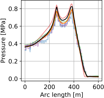
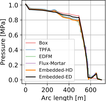
The employed embedded techniques enforce the continuity of the solution at the intersection of the matrix and fracture meshes. Hence, steep pressure jumps and barriers can not be represented. Consequently, for the embedded case we restrict our study to conductive fractures. In particular, we study the equi-dimensional embedded technique for 3, 5, and 6 levels of non-conforming mesh refinement (Section 2.6) performed exclusively in proximity of the fractures. This refinement patterns are generated automatically using the variational transfer algorithm for marking the elements of the matrix that are intersecting with the fractures. On Fig. 5, we plot the solution over the lines AA^′ (y = 0.75) and BB^′ (x = 0.5) and it can be observed that even for low resolutions, the solutions are in agreement with the reference results of Flemisch et al. 2018. From Table 2, it can be observed that with this particular set-up we reach an error in the order of $10^{-7}$ . Note that the number of elements in the fracture network do not influence the number of degrees of freedom, hence they do not count for the computational cost of solving the linear system but only for the set-up phase which is typically cheaper.

For the mortar method based experiment we are required to represent the fracture explicitly in the matrix mesh. For this particular scenario, the fracture is modelled as an equi-dimensional geometry which is meshed independently from the matrix. This allows us to refine all the different sub-domains in a completely independent manner and glue them together using the mortar method. We manually refine the matrix around the two fractures crossing at the center of the domain. This is done for having a higher resolution in the region of interest of the benchmark. From Table 2, it can be observed that even for low mesh resolutions of the matrix the error reaches an order of $10^{-8}$ for both, conductive and blocking fractures. However, the mesh resolution of the fractures is very high from the start. Despite this fact, in our experiments the actual degrees of freedom are only associated with one layer of nodes in the middle of the fracture, while the ones at the interface are eliminated by means of the mortar constraints as mention in Section 2.4.

We can observe that the embedded methodologies generate linear systems with comparable condition numbers and number of degrees of freedom. Whereas, the mortar-ED method gives rise to larger systems with larger condition numbers. Only with the mortar-ED we are able to solve the blocking scenario 4(b), however already for this simple experiment the mesh set-up is more laborious due to the matching geometry.

3.1.2 2D Benchmark Case 2: Hydrocoin

Table 3: Uniform refinement for the Embedded-ED vs Mortar-ED cases. Here

\textbf{err}_{m}

is the error computed with respect to the reference solution.

\#\textbf{UR}

refers to the number of uniform refinements.

Method	#-matr.	#-frac.	d.o.f.	nnz/size²	$\\|\cdot\\|_{2}$ -cond.	err_m	#UR
Embedded-ED	272 triangles	3 480	159	4.3e-2	2.9e9	5.1e-4	1
Embedded-ED	1 088 triangles	3 480	589	1.2e-2	1.1e10	8.5e-5	2
Embedded-ED	4 352 triangles	3 480	2 265	3.1e-2	4.3e10	1.7e-5	3
Embedded-ED	17 408 triangles	3 480	8 881	8.1e-4	1.8e11	4.0e-6	4
Embedded-ED	69 632 triangles	3 480	35 169	2.1e-4	6.8e11	1.9e-6	5
Embedded-ED	278 528 triangles	3 480	139 969	5.5e-5	2.7e12	1.3e-6	6
Mortar-ED	1 116 triangles	220	246	9.7e-3	3.6e6	2.1e-4	1
Mortar-ED	4 464 triangles	880	2 973	2.5e-3	7.6e6	1.9e-4	2
Mortar-ED	17 856 triangles	3520	11 285	6.4e-4	2.7e7	2.0e-4	3
Mortar-ED	71 424 triangles	14 080	43 941	1.7e-4	1.1e8	2.0e-4	4

(a) Uniform Refinement (UR)

(b) Adaptive Refinement (AR)

Figure 8: Pressure along line AA^′ for the uniform (A) and the adaptive (B) Embedded-ED test cases. Here, UR and AR refer to different steps of uniform and adaptive refinements performed on the initial matrix mesh. In particular, the number of AR are obtained combining a gradient recovery strategy with an adaptive refinement performed on the overlapping region between the matrix and the fracture zone. More details can be found in tables 4 and 3.

Table 4: Adaptive refinement for the Embedded-ED and Mortar-ED cases. Here,

\textbf{err}_{g}

is the threshold used for the gradient recovery strategy.

\#\textbf{AR}

refers to the number of adaptive refinements, whereas the number within parentheses refers to the steps of adaptive refinement performed on the overlapping region between the matrix and the fracture meshes.

Method	#-matr.	#-frac.	d.o.f.	nnz/size²	$\\|\cdot\\|_{2}$ -cond.	err_m	# AR	err_g
Embedded-ED	611 triangles	3 480	352	2.0e-2	1.5e10	8.9e-5	0 (2)	-
Embedded-ED	1 544 triangles	3 480	874	7.8e-3	5.3e10	1.6e-5	1 (2)	5
Embedded-ED	2 378 triangles	3 480	1354	4.5e-3	8.1e10	7.2e-5	2 (2)	5
Embedded-ED	7 913 triangles	3 480	4371	1.6e-3	3.5e11	2.9e-6	4 (2)	1
Embedded-ED	9 147 triangles	3 480	4991	1.5e-3	2.8e11	2.0e-6	4 (4)	1
Embedded-ED	21 599 triangles	3 480	11658	1.02e-3	1.06e12	1.4e-6	4 (6)	1
Mortar-ED	2 127 triangles	202	1375	5.9e-3	3.7e11	2.1e-4	1 (1)	5
Mortar-ED	8004 triangles	332	2791	1.1e-3	1.9e12	1.9e-4	2 (2)	5
Mortar-ED	19 515 triangles	442	10 600	7.1e-4	1.2e12	1.9e-4	3 (2)	5
Mortar-ED	28 692 triangles	457	15 284	4.8e-4	1.7e12	1.9e-4	4 (2)	5

(a) Uniform Refinement (UR)

(b) Adaptive Refinement (AR)

Figure 9: Pressure along line AA^′ for the uniform (A) and the adaptive (B) Mortar-ED test cases. Again, UR and AR refer to the steps of uniform and adaptive refinement performed on the initial matrix mesh. We use the MFD solution proposed in Flemisch et al. 2018 as a reference.

We test the capability of the adaptive mesh refinement by considering the hydrocoin benchmark [85] for two different techniques: the embedded-ED and the mortar-ED. The matrix consists of a rectangular box with a broken line located on the top, whereas the fracture network consists of two oblique lines. As shown in Fig. 6, we prescribe the piezometric head on the Dirichlet boundary on the top and Neumann no-flow on the remaining sides of the rectangular box. The permeability is set equal to $\mathbf{K}_{\gamma}=10^{-6}\,\text{[m/s]}$ for the fractures and $\mathbf{K}=10^{-8}\,\text{[m/s]}$ for the matrix. Fracture aperture is about $\epsilon_{1}=10.16$ for the left fracture and about $\epsilon_{2}=15$ for the right fracture.

We use a gradient recovery strategy for the a-posteriori error estimation to guide the adaptive refinement (AR) of the matrix and the fracture meshes, and compare the numerical results with those computed employing uniform refinement (UR). To this aim, we estimate the accuracy of each numerical simulation by computing the error with respect to the reference solution obtained by Flemisch et al. 2018 using a mimetic finite difference (MFD) method on a very fine mesh with $2\,260\,352$ triangles and $3\,471\,040$ dofs.

In Tables 3 and 4 we report the results related to the embedded-ED technique for UR and AR test cases, respectively. In particular, we specify the number of elements in the matrix mesh (#-matr.) and in the fracture mesh (#-frac.), the number of degrees of freedoms (d.o.f), the density of non zeros entries ( nnz/size²), the condition number ( $\|\cdot\|_{2}$ -cond), and the error computed with respect to the reference solution ( $\textbf{err}_{m}$ ). In Table 3 we also specify the number of uniform refinements ( $\#\textbf{UR}$ ), whereas in Table 4 we report the number of adaptive refinements ( $\#\textbf{AR}$ ), and the error-threshold used for the gradient recovery strategy ( $\textbf{err}_{g}$ ). We point out that both the UR and the AR strategies are only performed on the matrix mesh.

In Fig. 7 we show the meshes obtained for all the six AR test cases. The AR based on the gradient recovery strategy is combined with an AR perform ed on the overlapping region between the matrix and the fracture network. The number of AR performed in the overlapping zone are reported in Table 4 and specified within parentheses.

From the results summerized in Tables 3 and 4, we observe that the error $\textbf{err}_{m}$ progressively reduces by increasing the number of refinements. However, the adaptive strategy allows accurate results with coarser meshes when compared to the uniform technique. While a uniform refined mesh with more than $200\,000$ elements (#-matr.) is needed to get an error ( $\textbf{err}_{m}$ ) close to $10^{-6}$ , an adaptively refined mesh with a total number of elements ten times smaller ensures the same accuracy.

Fig. 8 shows the piezometric head obtained over line AA^′ for the UR (a) and the AR (b) test cases. One may note large discrepancies in the area of the left fracture, especially for the results referred to the uniform refined meshes. In this regard, we found that the a-posteriori error $\textbf{err}_{g}$ was higher close the sharp top boundary and in the zone occupied by the left fracture. Indeed, Fig. 7 (3)-(5) show that the AR strategy produces a mesh size reduction in such regions. Hence, all the AR test cases reveal a better agreement with the reference solution when compared to the UR scenarios.

For completeness, the numerical results obtained for the test case $3\,\text{AR}$ are presented in Fig. 6. Here, the colour refers to the spatial distribution of the piezometric head, whereas the contour lines are in black.

We perform the same analysis for the mortar-ED scenario and collect all the numerical results in Tables 3 and 4. Again, the use of AR allows us to achieve an accuracy comparable to the UR test cases with less elements in both the matrix mesh (#-matr.), and the fracture mesh (#-frac.).

In Fig. 9 we observe that the piezometric head profile computed along line AA^′ converges to the reference solution (MFD) by increasing the number of refinements for all the numerical simulations. We point out that, while the embedded-ED test cases reveal large discrepancies with respect to the reference solution in the region of the left fracture, only little differences are observed for the mortar-ED scenarios. Indeed, the mortar approach requires a matching geometry at the interface between fracture and matrix, and consequently more accurate results are achieved even with coarser meshes.

3.1.3 2D Benchmark Case 3: Realistic fracture network

We consider the same settings and reference solution used in Flemisch et al. 2018 Benchmark 4. For this benchmark, a more realistic fracture network is taken into consideration. Here, the size of the domain is 700 m x 600 m with a fracture network of 64 fractures divided in 13 connected groups. The matrix permeability is $\mathbf{K}=\mathbf{I}\cdot 10^{-14}\;$ m² All the fractures have the same permeability $10^{-8}\;$ m² and the same aperture $\epsilon=10^{-2}\;$ m. Hence, we have $\mathbf{K}_{\gamma^{1}}=\epsilon\mathbf{I}\cdot 10^{-8}$ for the HD case, and $\mathbf{K}_{\gamma^{2}}=\mathbf{I}\cdot 10^{-8}$ for the ED one. There are no-flow boundary conditions on top and bottom of the domain. A pressure of $1\,013\,250$ Pa is imposed on the left boundary and of 0 Pa on the right boundary. Due to the rather complex geometry of the fracture network, the mortar method is impractical, hence it is not used here. We exclusively present results for the equi-dimensional embedded method. The mesh of the matrix has been automatically refined at the intersection with the fracture, for each experiment with 3, 6, and 7 levels of non-conforming mesh refinement, respectively. It can be observed in Table 5 the condition numbers have comparable magnitudes for both HD and ED versions. The condition number becomes large with the extremely varying mesh size resulting from the heavily focused refinement around the fractures.

As can be observed in Fig. 10, the results obtained are similar to those obtained by other methods in the field although no reference solution is available. It can be noticed that the equi-dimensional variant is closer to the Box method compared to most other methods, including the hybrid dimensional results presented in [60]. From a practical perspective the equi-dimensional technique is slightly more complex since the fractures are extruded in normal direction, although automatically, thus requiring many more elements.

Table 5: Benchmark 4 in Flemisch et al. 2018. Mesh information, characteristics of system matrix and error in the matrix for the 2D Realistic fracture network benchmark in Embedded-ED and Embedded-HD cases.

Method	#-matr.	#-frac.	d.o.f.	nnz/size²	$\\|\cdot\\|_{2}$ -cond.
Embedded-ED	1405 quads	199 996	1487	1.9e-4	2.0e15
Embedded-ED	39 085 quads	199 996	41 773	2.3e-4	2.2e17
Embedded-ED	94 513 quads	199 996	102 486	9.1e-5	5.8e17
Embedded-HD	4200 quads	1024	4331	3.8e-3	1.3e16
Embedded-HD	67 200 quads	4096	67 721	1.6e-4	2.1e17

3.2 3D Experiments

Flow through fractured porous media is largely governed by 3D effects. Therefore, this section presents an application and evaluation of the dual Lagrange multiplier methods in 3D. First, results obtained with three Lagrange multiplier methods (embedded HD, embedded ED, mortar HD) are compared to results of $17$ methods presented in the benchmark study Berre et al. 2020. More complex benchmark cases in 3D are studied for the embedded HD method as part of the aforementioned benchmark study. The embedded HD method is preferably used for those geometrically complex cases as it eases meshing of the fracture networks and the porous matrix mesh can be chosen regular. Fracture network mesh generation for the embedded ED method is very challenging, which is particularly relevant at the fracture intersection. Furthermore, all 3D benchmark cases in Berre et al. 2020 are designed for very small fracture apertures and therefore equi-dimensional fracture meshes result in poor mesh quality. It is also important to bear in mind that equi-dimensional fracture meshes are mainly necessary for large aperture values and the benchmark cases yield no reason to use equi-dimensional meshes. Furthermore, the mortar method is less suited for complex fracture geometries due to the complexity of both, setting up the mesh and dealing with over-constrained scenarios for the mortar conditions. In a final realistic scenario the strength of each method is demonstrated and they are applied in a combined scenario as it could be typical for fractured systems.

3.2.1 3D Benchmark Case 1: Single fracture

In this section three Lagrange multiplier methods are compared to benchmark Case 1: Single Fracture presented by Berre et al. 2020, which already includes results obtained with the hybrid embedded method, presented in Schädle et al. 2019. Nevertheless, for completeness and for better comparison of the methods presented in this study the results of the hybrid embedded approach are again explicitly presented. To ease comparison, the results presented in the benchmark study are summarized and only the mean of all results as well as the standard deviation are plotted. The comparison of vastly different discretization methods is enabled by interpolating each solution to $1000$ evenly spaced points along a line. Following this, the mean and standard deviation are computed at each of these points. It is important to note that the mean of all results is not necessarily the correct solution and just provides a measure of comparison to the results presented in the aforementioned benchmark study. For the detailed benchmark results the interested reader is referred to Berre et al. 2020. Finally, improvements of the accuracy can be demonstrated for the embedded ED approach by adaptive mesh refinement.
Figure 11 shows the model domain of benchmark Case 1: Single Fracture which is adapted from Zielke et al. 1991 and Barlag et al. 1998. This case consists of a single fracture intersecting a matrix cube with $100\text{\,}\mathrm{m}$ edge length. The lowest $10\text{\,}\mathrm{m}$ thick layer of the matrix block (Matrix $2$ ) has an increased permeability. Fluid injection occurs at a Dirichlet boundary condition (BC ${}_{\text{1}}$ ) located above the fracture at the upper most $10\text{\,}\mathrm{m}$ thick layer of the matrix block. A Dirichlet boundary condition (BC ${}_{\text{2}}$ ) which acts as the outflow, is located at Matrix $2$ . The injection pressure is fixed at $4\text{\,}\mathrm{m}$ and the production pressure at $1\text{\,}\mathrm{m}$ . The permeability $\mathbf{K}$ in the Matrix $1$ is $\mathbf{I}\cdot 10^{-6}$ [m/s] and in the Matrix $2$ $\mathbf{I}\cdot 10^{-5}$ [m/s]. The fracture has a permeability $\mathbf{K}_{\gamma}$ of $\mathbf{I}_{\gamma}\cdot 10^{-3}$ [m/s] with an aperture $\epsilon$ of $10^{-2}$ [m].

The results obtained with the hybrid- and equi-dimensional embedded method and the hybrid mortar method are presented in Figure 12. In the upper part of the figure, three different mesh sizes ( $\sim$ 1k, $\sim$ 10k, and $\sim$ 100k matrix cells) are compared to $17$ methods presented in Berre et al. 2020. It is important to keep in mind that the hybrid-dimensional embedded results are also part of the benchmark results. The pressure solution for all methods is compared along the line AA^′ (see Fig. 11).
Overall, the results of the methods presented here and the methods presented in Berre et al. 2020 show good convergence towards a common solution. Particularly for the very coarse mesh of only $\sim$ 1k cells in the matrix domains the Lagrange multiplier methods show some deviations. These deviations are more pronounced for the embedded HD method at the first half of line AA^′ and for the embedded ED and the mortar method at the second half. The deviations are partially due to the fact that most of the other methods presented in the benchmark study represent the fracture geometry in the matrix explicitly in matching mesh geometries. Embedded techniques typically require a resolution that is roughly twice as high as fitted mesh techniques to achieve the same accuracy. Already for the case with $\sim$ 10k cells the embedded HD and ED methods show very similar results. For the coarsest case neither of the methods is preferable as they all show deviations in different regions. Furthermore, the solution of the mortar method shows a kink at $\sim$ $115\text{\,}\mathrm{m}$ for all mesh sizes. As mentioned above, this is due to over-constrained dofs, which poses significant technical challenges to be automated in 3D.
As shown in 3.1.2 adaptive mesh refinement allows to obtain more accurate results while reducing the number of matrix elements. Here the matrix mesh for the embedded ED approach is adaptively refined with up to two refinement steps, starting at $\sim$ 500 cells by progressively reducing the threshold of error adopted for the gradient recovery strategy. For brevity, we refer to the error threshold as $\mathbf{err}_{g}$ and to the number of adaptive refinement steps as AR. Thus, we employ $\mathbf{err}_{g}=$15$$ and $\text{AR}=\rm{1}$ for the coarsest mesh, $\mathbf{err}_{g}=$5$$ and $\text{AR}=$2$$ for the middle mesh, and $\mathbf{err}_{g}=$0.1$$ and $\text{AR}=$2$$ for the finest test case. One may note that the the error threshold, $\mathbf{err}_{g}$ , is progressively reduced to increase the accuracy of the numerical results. The matrix meshes resulting from the adaptive mesh refinement have $\sim$ 1.3k, $\sim$ 9k, and $\sim$ 28k cells. In Fig. 12, second row, we compare the results obtained with uniformly refined meshes with those obtained with adaptive mesh refinement. While the $\mathrm{amr}_{1}$ has some more cells than the compared uniform mesh, the pressure solution along parts of the line AA^′ is closer to the mean of all benchmark methods. For the two finer meshes, an improvement in accuracy is clearly visible. Taken together, all Lagrange multiplier methods presented here show good convergence and match well with other methods presented in the benchmark study.

Figure 12: Pressure results along the line AA^′ for

\sim

1k,

\sim

10k, and

\sim

100k matrix cells for uniform refinement (upper figure) and

\sim

1.3k,

\sim

9k, and

\sim

28k for adaptive mesh refinement (lower figure). Results are shown with uniform refinement for the hybrid-dimensional (HD) and equi-dimensional (ED) embedded method and the hybrid mortar method and with adaptive mesh refinement for the equi-dimensional embedded method. The black line shows the mean results of all benchmark methods and the grey range shows the standard deviation, respectively [83].

3.3 3D Realistic scenario

Geological setting with fractures and faults often require to represent such features with permeability and aperture ranging over several orders of magnitude. Therefore, their combined representation in numerical models is crucial for a complete description of geological settings. The setup of present realistic scenario is loosely based on the geological setting at the Grimsel Test Site, (GTS) [88]. However, it is important to note that the steady-state flow field, as computed here, is difficult to achieve in experiments conducted in such laboratories with a very low permeability rock matrix. Nevertheless, the given setup allows to demonstrate the different strength of the particular methods described in this study, i.e. complex fracture networks, fractures with large aperture widths, and blocking fractures. Even more importantly, this realistic scenario shows the integration of several coupling strategies in a single joint framework method.
Figure 13 shows the model domain with a complex fracture network (blue) located between two large features with two intersecting fractures each. One of these features acts as blocking fractures (yellow) with low permeability values, the fractures in the other feature have large apertures (magenta). Furthermore, two boreholes are drilled into the rock domain with one of them ending in the large aperture fractures and the other one in the rock domain. The upper right corner of the square domain is not modeled as it acts as an access tunnel with atmospheric pressure. Consequently, the pressure at the outer boundary is fixed by a Dirichlet boundary condition of $p_{D}=(x-y+100)\;0.025$ (green). This boundary condition results in a pressure of $1\text{\,}\mathrm{MPa}$ at the access tunnel location and $5\text{\,}\mathrm{MPa}$ at the lower right corner. At the top and bottom (z-direction) of the domain no-flow boundary conditions are applied.
In the numerical model the fractures and fracture network are represented by three different methods described above. The complex fracture network (blue) is meshed with lower-dimensional manifolds and embedded in the matrix mesh and has been initially presented by Schädle et al. 2019. In this study the fracture aperture and permeability and the matrix permeability are chosen so that the fractures and the matrix contribute similarly to the overall flow. In contrast, the rock matrix in the present experiment holds a low permeability and the fracture properties are chosen to dominate the flow. The fracture radius distribution in the network follows a power law, with truncations at $2.5\text{\,}\mathrm{m}$ and $10\text{\,}\mathrm{m}$ . The $150$ fractures are circular, randomly oriented, and distributed in a cubical area of the model domain with a side length of $25\text{\,}\mathrm{m}$ . The fracture aperture is $\sim 10^{-4}$ m and the permeability chosen to be $\sim 10^{-9}$ m ${}^{\text{2}}$ . Furthermore, the two fractures with large apertures (magenta) are represented by equi-dimensional domains embedded in the matrix domain. One of these fractures is intersected by a borehole which is explicitly meshed as a sub-domain. The two fractures are circular with an aperture width of $3\text{\times}{10}^{-1}\text{\,}\mathrm{m}$ and radii of $25\text{\,}\mathrm{m}$ . Further, the infilling material of these fractures is assumed to have a permeability of $1\text{\times}{10}^{-12}\text{\,}{\mathrm{m}}^{2}$ . In the borehole domain a forcing function of $1.0\text{\times}{10}^{-13}$ is applied in a volume of $1\text{\times}{10}^{-2}\text{\,}{\mathrm{m}}^{3}$ , acting as an injection borehole with a pressure of $\sim$ $5.5\text{\,}\mathrm{MPa}$ . To represent fractures with low permeability, acting as blocking fractures, two fractures (yellow) are described by equi-dimensional domains coupled to the matrix mesh by the mortar method. These fractures are rectangular with a side length of $35\text{\,}\mathrm{m}$ and permeability of $1\text{\times}{10}^{-21}\text{\,}{\mathrm{m}}^{2}$ . Generally, the shape of the fractures might of any shape, e.g. circular or rectangular. The second borehole acts as a sink with a fixed atmospheric pressure. This borehole is described by a mortar coupling of a small domain with the dimensions of the borehole and a fixed pressure of $1\text{\,}\mathrm{MPa}$ . Finally, the matrix permeability is $1\text{\times}{10}^{-18}\text{\,}{\mathrm{m}}^{2}$ .

Figure 14 shows the pressure distribution across three planes intersecting the model domain parallel to the xy-plane. Throughout all planes the low permeability fractures act as discontinuities for pressure. Moreover, for plane (a) a clear discontinuity can be observed across the two fracture cross sections. With the high aperture and permeability of the complex fracture network and the low permeability of the rock matrix the pressure across the fracture network is equilibrated, connecting the upper right with the lower left part of the domain. With the injection borehole in one of the two equi-dimensional fractures, these fractures and the surrounding rock matrix area subject to the largest pressure values. In plane (b) the production borehole locally reduces the pressure to atmospheric pressure. However, due to the low permeability of the rock matrix the gradient around this borehole is very steep and the influence on the overall solution is limited. Additionally, the fixed pressure boundary condition at the outer boundary forces the pressure to steep gradients close to the embedded ED fractures with high injection pressure. These steep gradients result from boundary effects and for a representative study of such a geological setting the domain would have to be extended in these areas. However, the goal of this study is to demonstrate the application of Lagrange multipliers for different coupling strategies, spanning from equi-dimensional to lower dimensional models, and from embedded to mortar techniques. Ultimately allowing for more flexibility in the treatment of the fracture and matrix configuration. Furthermore, such steep gradients are generally difficult to resolve in numerical models, thus adding further complexity to this test case. In summary, this realistic scenario demonstrates the strength of each method and the ability of the presented unified framework to combine all of these approaches while yielding smooth pressure results in geologically complex settings. More specifically, the hybrid-dimensional embedded approach eases meshing of complex fracture networks of fractures with small aperture widths, the equi-dimensional embedded approach allows to consider fractures with large aperture widths, and the equi-dimensional mortar approach enables to consider blocking fractures.

4 Conclusion

This study expands on previous works based on the application of the Lagrange multiplier method to compute single-phase fluid flow problems in fracture dominated porous media. In particular, we employ the finite element method in combination with an $L^{2}$ -projection operator to couple different types of non-conforming meshes. The non-conformity might arise at the interface of independently meshed sub-domains, at hanging nodes resulting from adaptive mesh refinement, or by combining multiple overlapping meshes. Furthermore, fractures are either described by equi-dimensional or hybrid-dimensional domains. The applied Lagrange multiplier is discretized using dual basis functions, which provide two main advantages. First, the number of degrees of freedom is reduced to the ones of the background mesh representing the porous-matrix. Second, the arising symmetric-positive-definite linear systems are convenient work with.
Here, we present a unified framework covering all coupling techniques mentioned above. The different mesh solutions are compared with state-of-the-art benchmark cases in 2D and 3D, the numerical performance is studied, and use cases are presented in isolation and combination. Overall, the results suggest that the presented tool-set is capable of computing fluid-flow through complex and heterogeneous rock formations in a robust and convenient way. It is important to bear in mind that realistic scenarios of fracture dominated rock formations may include fractures with geometric and physical properties ranging over many orders of magnitude. Therefore, the presented single joint framework allows to deeply exploit non-conforming hybrid- and equi-dimensional fracture models and efficiently combine these models. By using the dual Lagrange multiplier we are able to combine multiple complex fracture networks without changing the size of the algebraic system arising from the porous-medium matrix, although we have more non-zero entries associated with the coupled degrees of freedom. It is also worth to point out that the conditioning of the system is not worsened, as it is the case when using other types of Lagrange multipliers [60].
With the integration of adaptive mesh refinement in the solution process, the error in the solution can be controlled in an automated way either by means of an error estimator or by pre-defining areas of interest for refinement. This allowed to complement the discussion in Schädle et al. 2019 about the necessity of having a finer mesh around fractures and their tips and intersections.
The study of a realistic geological setting, inspired by the Grimsel Test Site, demonstrates the advantage of the unified framework to represent vastly different fracture geometries and properties within a single numerical model. This allows to expand on existing numerical studies of such systems by the opportunity to include a large range of fracture representations. Furthermore, the highly efficient and convenient tools combined with the eased meshing of non-conforming meshes enables stochastic studies for a wide range of fracture dominated systems.
Further investigations based on this unified framework would benefit by focusing on mass conservation properties of the finite element discretization and application to transport problems.

Acknowledgment

P.Z., M.G.C.N., and L.K. thank the SCCER-SoE and SCCER-FURIES programs, and the PASC project FASTER: Forecasting and Assessing Seismicity and Thermal Evolution in geothermal Reservoirs. P.S. thanks the Werner Siemens Foundation for their endowment of the Geothermal Energy and Geofluids group at the Institute of Geophysics, ETH Zurich.

Authorship statement

P.Z. lead the drafting of the manuscript, implemented most methods and numerical tools, developed parts of the conceptual models, and lead parts of the numerical experiments. P.S. contributed drafting the manuscript, lead the development of the 3D conceptual models, their validation, and presentation of the results. L.K. produced, collected, and prepared most of the 2D benchmark results. M.G.C.N contributed drafting the manuscript, implemented the adaptive refinement strategy and its integration with the variational transfer, lead the numerical experiments related to the adaptive refinement, and contributed to the 2D and 3D numerical experiments.

Conflict of interest

The authors declare that they have no conflict of interest.

Computer Code Availability

All methods and routines, used for this study, are implemented with the open-source software library Utopia [79]. Utopia’s lead developer is author Patrick Zulian at USI Lugano, Switzerland. The contact address and e-mail of Patrick Zulian are as follows:

Institute of Computational Science
Università della Svizzera italiana (USI - University of Lugano)
Via Giuseppe Buffi 13
CH-6900 Lugano
patrick.zulian@usi.ch

Utopia was first available in 2016, the programming language is C++ and it can be accessed through a git repository or a docker container on:

https://bitbucket.org/zulianp/utopia (approx. 40 MB of uncompressed data),
https://hub.docker.com/r/utopiadev/utopia.

The software dependencies are as follows:

PETSc (https://www.mcs.anl.gov/petsc),
must be compiled with MUMPS enabled
libMesh for the FE module (https://github.com/libMesh)

There are no hardware requirements given by Utopia. Potential hardware or software requirements of the underlying libraries libMesh and PETSc are not stated here.

References

Pochon et al. [2008] Alain Pochon, Jean-Pierre Tripet, Ronald Kozel, Benjamin Meylan, Michael Sinreich, and François Zwahlen. Groundwater protection in fractured media: a vulnerability-based approach for delineating protection zones in switzerland. Hydrogeology Journal, 16(7), 2008. doi: 10.1007/s10040-008-0323-0.
Read et al. [2013] T. Read, O. Bour, V. Bense, T. Le Borgne, P. Goderniaux, M.V. Klepikova, R. Hochreutener, N. Lavenant, and V. Boschero. Characterizing groundwater flow and heat transport in fractured rock using fiber-optic distributed temperature sensing. Geophysical Research Letters, 40(10):2055–2059, 2013. doi: 10.1002/grl.50397.
Tester et al. [2006] Jefferson W Tester, B Anderson, A Batchelor, D Blackwell, Ronald DiPippo, E Drake, John Garnish, B Livesay, Michal C Moore, Kenneth Nichols, et al. The future of geothermal energy: Impact of enhanced geothermal systems (egs) on the united states in the 21st century. Massachusetts Institute of Technology, 209, 2006.
McClure and Horne [2014] Mark W. McClure and Roland N. Horne. Correlations between formation properties and induced seismicity during high pressure injection into granitic rock. Engineering Geology, 175:74–80, 2014. ISSN 0013-7952. doi: http://dx.doi.org/10.1016/j.enggeo.2014.03.015.
Bond et al. [2003] Clare E. Bond, Ruth Wightman, and Philip S. Ringrose. The influence of fracture anisotropy on co2 flow. Geophysical Research Letters, 40(7):1284–1289, 2003. doi: 10.1002/grl.50313. URL https://agupubs.onlinelibrary.wiley.com/doi/abs/10.1002/grl.50313.
Bonnet et al. [2001] E. Bonnet, O. Bour, N. E. Odling, P. Davy, I. Main, P. Cowie, and B. Berkowitz. Scaling of fracture systems in geological media. Reviews of Geophysics, 39(3):347–383, 8 2001. ISSN 8755-1209. doi: 10.1029/1999RG000074. URL http:https://doi.org/10.1029/1999RG000074.
Rasmuson and Neretnieks [1986] Anders Rasmuson and Ivars Neretnieks. Radionuclide transport in fast channels in crystalline rock. Water Resources Research, 22(8):1247–1256, 1986.
Amann et al. [2018a] Florian Amann, Valentin Gischig, Keith Evans, Joseph Doetsch, Reza Jalali, Benoît Valley, Hannes Krietsch, Nathan Dutler, Linus Villiger, Bernard Brixel, et al. The seismo-hydromechanical behavior during deep geothermal reservoir stimulations: open questions tackled in a decameter-scale in situ stimulation experiment. Solid Earth, 9(1):115–137, 2018a.
de Dreuzy et al. [2012] Jean-Raynald de Dreuzy, Yves Méheust, and Géraldine Pichot. Influence of fracture scale heterogeneity on the flow properties of three-dimensional discrete fracture networks (dfn). Journal of Geophysical Research: Solid Earth, 117(B11), 2012.
Zimmerman et al. [1991] R.W. Zimmerman, S. Kumar, and G.S. Bodvarsson. Lubrication theory analysis of the permeability of rough-walled fractures. International Journal of Rock Mechanics and Mining Sciences & Geomechanics Abstracts, 28(4):325–331, 1991. ISSN 0148-9062. doi: https://doi.org/10.1016/0148-9062(91)90597-F. URL http://www.sciencedirect.com/science/article/pii/014890629190597F.
Ebigbo et al. [2016] Anozie Ebigbo, Philipp S Lang, Adriana Paluszny, and Robert W Zimmerman. Inclusion-based effective medium models for the permeability of a 3d fractured rock mass. Transport in Porous Media, 113(1):137–158, 2016.
Vogler et al. [2016] Daniel Vogler, Florian Amann, Peter Bayer, and Derek Elsworth. Permeability evolution in natural fractures subject to cyclic loading and gouge formation. Rock Mechanics and Rock Engineering, 49:3463–3479, 2016. doi: https://doi.org/10.1007/s00603-016-1022-0.
Neuman [1997] Shlomo P. Neuman. Stochastic approach to subsurface flow and transport: a view to the future, pages 231–241. International Hydrology Series. Cambridge University Press, 1997. doi: 10.1017/CBO9780511600081.016.
Berkowitz [2002] Brian Berkowitz. Characterizing flow and transport in fractured geological media: A review. Advances in Water Resources, 25(8):861–884, 2002. doi: 10.1016/S0309-1708(02)00042-8.
Cacas et al. [1990] M. C. Cacas, E. Ledoux, G. Marsily, B. Tillie, A. Barbreau, E. Durand, B. Feuga, and P. Peaudecerf. Modeling fracture flow with a stochastic discrete fracture network: calibration and validation: 1. the flow model. Water Resources Research, 26(3):479–489, 3 1990. ISSN 0043-1397. doi: 10.1029/WR026i003p00479. URL https://doi.org/10.1029/WR026i003p00479.
Hobé et al. [2018] Alex Hobé, Daniel Vogler, Martin P. Seybold, Anozie Ebigbo, Randolph R. Settgast, and Martin O. Saar. Estimating fluid flow rates through fracture networks using combinatorial optimization. Advances in Water Resources, 122:85–97, 2018. ISSN 0309-1708. doi: https://doi.org/10.1016/j.advwatres.2018.10.002. URL http://www.sciencedirect.com/science/article/pii/S0309170818300666.
Neuman [2005] Shlomo P Neuman. Trends, prospects and challenges in quantifying flow and transport through fractured rocks. Hydrogeology Journal, 13(1):124–147, 2005.
de Dreuzy et al. [2013] Jean-Raynald de Dreuzy, Géraldine Pichot, Baptiste Poirriez, and Jocelyne Erhel. Synthetic benchmark for modeling flow in 3d fractured media. Computers & Geosciences, 50:59–71, 2013.
Dessirier et al. [2018] Benoît Dessirier, Chin-Fu Tsang, and Auli Niemi. A new scripting library for modeling flow and transport in fractured rock with channel networks. Computers & Geosciences, 111:181–189, 2018.
Warren and Root [1963] J.E. Warren and P.J. Root. The Behavior of Naturally Fractured Reservoirs. Society of Petroleum Engineers Journal, 3(3):245–255, sep 1963. ISSN 0197-7520. doi: 10.2118/426-PA. URL https://www.onepetro.org/download/journal-paper/SPE-426-PA?id=journal-paper{%}2FSPE-426-PAhttp://www.onepetro.org/doi/10.2118/426-PA.
Barenblatt et al. [1960] GI Barenblatt, Iu P Zheltov, and IN Kochina. Basic concepts in the theory of seepage of homogeneous liquids in fissured rocks strata. Journal of applied mathematics and mechanics, 24(5):1286–1303, 1960.
Kazemi [1969] Hossein Kazemi. Pressure transient analysis of naturally fractured reservoirs with uniform fracture distribution. Society of petroleum engineers Journal, 9(04):451–462, 1969.
Kazemi et al. [1976] H Kazemi, LS Merrill Jr, KL Porterfield, PR Zeman, et al. Numerical simulation of water-oil flow in naturally fractured reservoirs. Society of Petroleum Engineers Journal, 16(06):317–326, 1976.
Noorishad and Mehran [1982] Jahan Noorishad and Mohsen Mehran. An upstream finite element method for solution of transient transport equation in fractured porous media. Water Resources Research, 18(3):588–596, 6 1982. ISSN 0043-1397. doi: 10.1029/WR018i003p00588. URL https://doi.org/10.1029/WR018i003p00588.
Baca et al. [1984] R. G. Baca, R. C. Arnett, and D. W. Langford. Modelling fluid flow in fractured-porous rock masses by finite-element techniques. International Journal for Numerical Methods in Fluids, 4(4):337–348, 4 1984. ISSN 1097-0363. doi: 10.1002/fld.1650040404. URL https://doi.org/10.1002/fld.1650040404.
Hyman et al. [2015] Jeffrey D Hyman, Satish Karra, Nataliia Makedonska, Carl W Gable, Scott L Painter, and Hari S Viswanathan. dfnworks: A discrete fracture network framework for modeling subsurface flow and transport. Computers & Geosciences, 84:10–19, 2015.
Flemisch et al. [2011] Bernd Flemisch, Melanie Darcis, K Erbertseder, B Faigle, A Lauser, Klaus Mosthaf, S Müthing, Philipp Nuske, A Tatomir, M Wolff, and Helmig Rainer. Dumux: Dune for multi- $\{$ phase, component, scale, physics,… $\}$ flow and transport in porous media. Advances in Water Resources, 34(9):1102–1112, 2011. doi: 10.1016/j.advwatres.2011.03.007.
Lipnikov et al. [2014] Konstantin Lipnikov, Gianmarco Manzini, and Mikhail Shashkov. Mimetic finite difference method. Journal of Computational Physics, 257:1163–1227, 2014. doi: 10.1016/j.jcp.2013.07.031.
Lee and Ni [2015] I-Hsien Lee and Chuen-Fa Ni. Fracture-based modeling of complex flow and co2 migration in three-dimensional fractured rocks. Computers & geosciences, 81:64–77, 2015.
Lee et al. [2019] I-Hsien Lee, Chuen-Fa Ni, Fang-Pang Lin, Chi-Ping Lin, and Chien-Chung Ke. Stochastic modeling of flow and conservative transport in three-dimensional discrete fracture networks. Hydrology and Earth System Sciences, 23(1):19–34, 2019. doi: 10.5194/hess-23-19-2019.
Cacace and Blöcher [2015] Mauro Cacace and Guido Blöcher. Meshit—a software for three dimensional volumetric meshing of complex faulted reservoirs. Environmental Earth Sciences, 74(6):5191–5209, 2015.
Holm et al. [2006] Randi Holm, Roland Kaufmann, Bjørn-Ove Heimsund, Erlend Øian, and Magne S Espedal. Meshing of domains with complex internal geometries. Numerical Linear Algebra with Applications, 13(9):717–731, 2006.
Blessent et al. [2009] Daniela Blessent, René Therrien, and Kerry MacQuarrie. Coupling geological and numerical models to simulate groundwater flow and contaminant transport in fractured media. Computers & Geosciences, 35(9):1897–1906, 2009.
Karimi-Fard et al. [2004] M. Karimi-Fard, L.J. Durlofsky, and K. Aziz. An efficient discrete-fracture model applicable for general-purpose reservoir simulators. SPE Journal, 9(2):227–236, 2004.
Bogdanov et al. [2003] II Bogdanov, VV Mourzenko, J-F Thovert, and PM Adler. Two-phase flow through fractured porous media. Physical Review E, 68(2):026703, 2003.
Monteagudo and Firoozabadi [2004] JEP Monteagudo and Abbas Firoozabadi. Control-volume method for numerical simulation of two-phase immiscible flow in two-and three-dimensional discrete-fractured media. Water resources research, 40(7), 2004.
Helmig et al. [1997] Rainer Helmig et al. Multiphase flow and transport processes in the subsurface: a contribution to the modeling of hydrosystems. Springer-Verlag, 1997.
Flemisch et al. [2018] Bernd Flemisch, Inga Berre, Wietse Boon, Alessio Fumagalli, Nicolas Schwenck, Anna Scotti, Ivar Stefansson, and Alexandru Tatomir. Benchmarks for single-phase flow in fractured porous media. Advances in Water Resources, 111:239–258, 2018. ISSN 0309-1708. doi: https://doi.org/10.1016/j.advwatres.2017.10.036. URL http://www.sciencedirect.com/science/article/pii/S0309170817300143.
Keilegavlen et al. [2019] Eirik Keilegavlen, Runar Berge, Alessio Fumagalli, Michele Starnoni, Ivar Stefansson, Jhabriel Varela, and Inga Berre. Porepy: An open-source software for simulation of multiphysics processes in fractured porous media. arXiv preprint arXiv:1908.09869, 2019.
Nordbotten et al. [2019] Jan Martin Nordbotten, Wietse M Boon, Alessio Fumagalli, and Eirik Keilegavlen. Unified approach to discretization of flow in fractured porous media. Computational Geosciences, 23(2):225–237, 2019. doi: 10.1007/s10596-018-9778-9.
Devloo et al. [2019] Philippe Devloo, Wenchao Teng, and Chen-Song Zhang. Multiscale hybrid-mixed finite element method for flow simulation in fractured porous media. Computer Modeling in Engineering & Sciences, 119(1):145–163, 2019. doi: 10.32604/cmes.2019.04812.
Duran et al. [2019] Omar Duran, Philippe R B Devloo, Sônia M Gomes, and Frédéric Valentin. A multiscale hybrid method for darcy’s problems using mixed finite element local solvers. Computer Methods in Applied Mechanics and Engineering, 354:213–244, 2019. doi: 10.1016/j.cma.2019.05.013.
Brenner et al. [2016a] Konstantin Brenner, Mayya Groza, Cindy Guichard, Gilles Lebeau, and Roland Masson. Gradient discretization of hybrid dimensional darcy flows in fractured porous media. Numerische Mathematik, 134(3):569–609, 2016a. doi: 10.1007/s00211-015-0782-x.
Brenner et al. [2016b] Konstantin Brenner, Julian Hennicker, Roland Masson, and Pierre Samier. Gradient discretization of hybrid-dimensional darcy flow in fractured porous media with discontinuous pressures at matrix–fracture interfaces. IMA Journal of Numerical Analysis, 37(3):1551–1585, 2016b. doi: 10.1093/imanum/drw044.
Facciolà et al. [2019] Chiara Facciolà, Paola Francesca Antonietti, and Marco Verani. Mixed-primal discontinuous galerkin approximation of flows in fractured porous media on polygonal and polyhedral grids. PAMM, 19(1):e201900117, 2019.
Li and Lee [2008] Liyong Li and Seong H Lee. Efficient field-scale simulation of black oil in a naturally fractured reservoir through discrete fracture networks and homogenized media. SPE Reservoir Evaluation & Engineering, 11(04):750–758, 2008.
Hajibeygi et al. [2011] Hadi Hajibeygi, Dimitrios C. Karvounis, and Patrick Jenny. A hierarchical fracture model for the iterative multiscale finite volume method. Journal of Computational Physics, 230(24):8729–8743, 2011. ISSN 00219991. doi: 10.1016/j.jcp.2011.08.021.
Ţene et al. [2017] Matei Ţene, Sebastian BM Bosma, Mohammed Saad Al Kobaisi, and Hadi Hajibeygi. Projection-based embedded discrete fracture model (pedfm). Advances in Water Resources, 105:205–216, 2017.
Moinfar et al. [2014] Ali Moinfar, Abdoljalil Varavei, Kamy Sepehrnoori, and Russell T. Johns. Development of an Efficient Embedded Discrete Fracture Model for 3D Compositional Reservoir Simulation in Fractured Reservoirs. SPE Journal, 19(02):289–303, apr 2014. ISSN 1086-055X. doi: 10.2118/154246-PA. URL http://www.onepetro.org/doi/10.2118/154246-PA.
Nikitin and Yanbarisov [2020] Kirill D Nikitin and Ruslan M Yanbarisov. Monotone embedded discrete fractures method for flows in porous media. Journal of Computational and Applied Mathematics, 364:112353, 2020. doi: 10.1016/j.cam.2019.112353.
Flemisch et al. [2016] Bernd Flemisch, Alessio Fumagalli, and Anna Scotti. A Review of the XFEM-Based Approximation of Flow in Fractured Porous Media. In Advances in Discretization Methods, pages 47–76. Springer International Publishing, 2016. doi: 10.1007/978-3-319-41246-7_3. URL http://link.springer.com/10.1007/978-3-319-41246-7{_}3.
Xu and Yang [2020] Ziyao Xu and Yang Yang. The hybrid dimensional representation of permeability tensor: A reinterpretation of the discrete fracture model and its extension on nonconforming meshes. Journal of Computational Physics, 415:109523, 2020. doi: https://doi.org/10.1016/j.jcp.2020.109523.
Capatina et al. [2016] D Capatina, R Luce, H El-Otmany, and N Barrau. Nitsche’s extended finite element method for a fracture model in porous media. Applicable Analysis, 95(10):2224–2242, 2016.
Huang et al. [2011] Hao Huang, Ted A Long, Jing Wan, and William P Brown. On the use of enriched finite element method to model subsurface features in porous media flow problems. Computational Geosciences, 15(4):721–736, 2011.
Schwenck et al. [2015] Nicolas Schwenck, Bernd Flemisch, Rainer Helmig, and Barbara I. Wohlmuth. Dimensionally reduced flow models in fractured porous media: crossings and boundaries. Computational Geosciences, 19(6):1219–1230, dec 2015. ISSN 1420-0597. doi: 10.1007/s10596-015-9536-1. URL http://link.springer.com/10.1007/s10596-015-9536-1.
D’Angelo and Scotti [2012] Carlo D’Angelo and Anna Scotti. A mixed finite element method for darcy flow in fractured porous media with non-matching grids. ESAIM: Mathematical Modelling and Numerical Analysis, 46(2):465–489, 2012.
Fumagalli and Scotti [2013] Alessio Fumagalli and Anna Scotti. A numerical method for two-phase flow in fractured porous media with non-matching grids. Advances in Water Resources, 62:454–464, 2013.
Fumagalli et al. [2019] Alessio Fumagalli, Eirik Keilegavlen, and Stefano Scialò. Conforming, non-conforming and non-matching discretization couplings in discrete fracture network simulations. Journal of Computational Physics, 376:694–712, 2019.
Köppel et al. [2018] M. Köppel, V. Martin, J. Jaffré, and Jean E Roberts. A lagrange multiplier method for a discrete fracture model for flow in porous media. Computational Geosciences, 23(2):239–253, 2018.
Schädle et al. [2019] Philipp Schädle, Patrick Zulian, Daniel Vogler, Sthavishtha R. Bhopalam, Maria G.C. Nestola, Anozie Ebigbo, Rolf Krause, and Martin O. Saar. 3d non-conforming mesh model for flow in fractured porous media using lagrange multipliers. Computers & Geosciences, 132:42 – 55, 2019. ISSN 0098-3004. doi: https://doi.org/10.1016/j.cageo.2019.06.014. URL http://www.sciencedirect.com/science/article/pii/S0098300418312032.
Berre et al. [2018] Inga Berre, Florian Doster, and Eirik Keilegavlen. Flow in fractured porous media: A review of conceptual models and discretization approaches. Transport in Porous Media, pages 1–22, 2018.
Nestola et al. [2019] Maria Giuseppina Chiara Nestola, Barna Becsek, Hadi Zolfaghari, Patrick Zulian, Dario De Marinis, Rolf Krause, and Dominik Obrist. An immersed boundary method for fluid-structure interaction based on variational transfer. Journal of Computational Physics, 398:108884, 2019. ISSN 0021-9991. doi: https://doi.org/10.1016/j.jcp.2019.108884. URL http://www.sciencedirect.com/science/article/pii/S0021999119305820.
Osborn et al. [2018] Sarah Osborn, Patrick Zulian, Thomas Benson, Umberto Villa, Rolf Krause, and Panayot S. Vassilevski. Scalable hierarchical pde sampler for generating spatially correlated random fields using nonmatching meshes. Numerical Linear Algebra with Applications, 25(3):e2146, 2018. doi: 10.1002/nla.2146. URL https://onlinelibrary.wiley.com/doi/abs/10.1002/nla.2146.
Glowinski et al. [1994] Roland Glowinski, Tsorng-Whay Pan, and Jacques Periaux. A fictitious domain method for dirichlet problem and applications. Computer Methods in Applied Mechanics and Engineering, 111(3-4):283–303, 1994.
Bernardi et al. [1993] Christine Bernardi, Yvon Maday, and Anthony T Patera. Domain decomposition by the mortar element method. In Asymptotic and numerical methods for partial differential equations with critical parameters, pages 269–286. Springer, 1993.
Popp et al. [2012] Alexander Popp, Barbara I Wohlmuth, Michael W Gee, and Wolfgang A Wall. Dual quadratic mortar finite element methods for 3d finite deformation contact. SIAM Journal on Scientific Computing, 34(4):B421–B446, 2012.
Von Planta et al. [2019] Cyrill Von Planta, Daniel Vogler, Xiaoqing Chen, Maria GC Nestola, Martin O Saar, and Rolf Krause. Simulation of hydro-mechanically coupled processes in rough rock fractures using an immersed boundary method and variational transfer operators. Computational Geosciences, 23(5):1125–1140, 2019.
Frih et al. [2012] Najla Frih, Vincent Martin, Jean Elizabeth Roberts, and Ali Saâda. Modeling fractures as interfaces with nonmatching grids. Computational Geosciences, 16(4):1043–1060, sep 2012. doi: 10.1007/s10596-012-9302-6. URL http://link.springer.com/10.1007/s10596-012-9302-6.
Boon et al. [2018] Wietse M Boon, Jan M Nordbotten, and Ivan Yotov. Robust discretization of flow in fractured porous media. SIAM Journal on Numerical Analysis, 56(4):2203–2233, 2018.
Hesch et al. [2014] C. Hesch, A.J. Gil, A. Arranz Carre no, J. Bonet, and P. Betsch. A mortar approach for fluid–structure interaction problems: Immersed strategies for deformable and rigid bodies. Computer Methods in Applied Mechanics and Engineering, 278:853 – 882, 2014. ISSN 0045-7825. doi: https://doi.org/10.1016/j.cma.2014.06.004. URL http://www.sciencedirect.com/science/article/pii/S0045782514001893.
Wohlmuth [2000] Barbara I Wohlmuth. A mortar finite element method using dual spaces for the lagrange multiplier. SIAM journal on numerical analysis, 38(3):989–1012, 2000.
Briggs and McCormick [2000] William L Briggs and Steve F McCormick. A multigrid tutorial, volume 72. Siam, 2000.
Lamichhane et al. [2005] Bishnu P Lamichhane, Rob P Stevenson, and Barbara I Wohlmuth. Higher order mortar finite element methods in 3d with dual lagrange multiplier bases. Numerische Mathematik, 102(1):93–121, 2005.
Paz and Leigh [2001] Mario Paz and William Leigh. Static condensation and substructuring. In Integrated Matrix Analysis of Structures, pages 239–260. Springer, 2001.
Krause et al. [2015] Dorian Krause, Thomas Dickopf, Mark Potse, and Rolf Krause. Towards a large-scale scalable adaptive heart model using shallow tree meshes. Journal of Computational Physics, 298:79 – 94, 2015. ISSN 0021-9991. doi: https://doi.org/10.1016/j.jcp.2015.05.005. URL http://www.sciencedirect.com/science/article/pii/S002199911500323X.
Farah et al. [2018] P. Farah, W. A. Wall, and A. Popp. A mortar finite element approach for point, line, and surface contact. International Journal for Numerical Methods in Engineering, 114(3):255–291, 2018. doi: 10.1002/nme.5743. URL https://onlinelibrary.wiley.com/doi/abs/10.1002/nme.5743.
Sutherland and Hodgman [1974] Ivan E Sutherland and Gary W Hodgman. Reentrant polygon clipping. Communications of the ACM, 17(1):32–42, 1974.
Červený et al. [2019] Jakub Červený, Veselin Dobrev, and Tzanio Kolev. Non-conforming mesh refinement for high-order finite elements, 2019.
Zulian et al. [2016] Patrick Zulian, Alena Kopaničáková, Maria Chiara Giuseppina Nestola, Andreas Fink, Nur Fadel, Victor Magri, Teseo Schneider, and Eric Botter. Utopia: A C++ embedded domain specific language for scientific computing. Git repository. https://bitbucket.org/zulianp/utopia, 2016. URL https://bitbucket.org/zulianp/utopia.
Kirk et al. [2006] B. S. Kirk, J. W. Peterson, R. H. Stogner, and G. F. Carey. libMesh: A C++ Library for Parallel Adaptive Mesh Refinement/Coarsening Simulations. Engineering with Computers, 22(3–4):237–254, 2006.
Zulian [2016] Patrick Zulian. ParMOONoLith: parallel intersection detection and automatic load-balancing library. Git repository. https://bitbucket.org/zulianp/par_moonolith, 2016. URL https://bitbucket.org/zulianp/par_moonolith.
Balay et al. [1997] Satish Balay, William D. Gropp, Lois Curfman McInnes, and Barry F. Smith. Efficient management of parallelism in object oriented numerical software libraries. In E. Arge, A. M. Bruaset, and H. P. Langtangen, editors, Modern Software Tools in Scientific Computing, pages 163–202. Birkhäuser Press, 1997.
Berre et al. [2020] Inga Berre, Wietse M Boon, Bernd Flemisch, Allessio Fumagalli, Dennis Gläser, Eirik Keilegavlen, Anna Scotti, Ivar Stefansson, Alexandru Tatomir, Konstantin Brenner, Samuel Burbulla, Philippe Devloo, Omar Duran, Marco Favino, Julian Hennicker, I-Hsien Lee, Konstantin Lipnikov, Roland Masson, Klaus Mosthaf, Maria Giuseppina Chiara Nestola, Chuen-Fa Ni, Kirill Nikitin, Philipp Schädle, Daniil Svyatskiy, Ruslan Yanbarisov, and Patrick Zulian. Verification benchmarks for single-phase flow in three-dimensional fractured porous media. arXiv preprint arXiv:2002.07005, 2020.
Yan and Zhou [2001] Ningning Yan and Aihui Zhou. Gradient recovery type a posteriori error estimates for finite element approximations on irregular meshes. Computer methods in applied mechanics and engineering, 190(32-33):4289–4299, 2001.
Nicholson et al. [1987] Thomas J Nicholson, TJ McCartin, Paul A Davis, and Walt Beyeler. Nrc experiences in hydrocoin: An international project for studying ground-water flow modeling strategies. In Waste management’87: Waste isolation in the US, technical programs, and public education. 1987.
Zielke et al. [1991] W Zielke, R Helmig, K P Krohn, H Shao, and J Wollrath. Discrete modelling of transport processes in fractured porous rock. In 7th ISRM Congress. International Society for Rock Mechanics and Rock Engineering, 1991.
Barlag et al. [1998] C Barlag, R Hinkelmann, R Helmig, and W Zielke. Adaptive methods for modelling transport processes in fractured subsurface systems. In 3rd International Conference on Hydroscience and Engineering, Cottbus, Center of Computational Hydroscience and Engineering, The University of Mississippi, volume 284, 1998.
Amann et al. [2018b] F. Amann, V. Gischig, K. Evans, J. Doetsch, R. Jalali, B. Valley, H. Krietsch, N. Dutler, L. Villiger, B. Brixel, M. Klepikova, A. Kittilä, C. Madonna, S. Wiemer, M. O. Saar, S. Loew, T. Driesner, H. Maurer, and D. Giardini. The seismo-hydromechanical behavior during deep geothermal reservoir stimulations: open questions tackled in a decameter-scale in situ stimulation experiment. Solid Earth, 9(1):115–137, 2018b. doi: 10.5194/se-9-115-2018.