Provable More Data Hurt in High Dimensional Least Squares Estimator

Zeng Li Affiliation: Department of Statistics and Data Science Affiliation: Southern University of Science and Technology Affiliation: Shenzhen, China Email: liz9@sustech.edu.cn Chuanlong Xie Affiliation: Huawei Noah’s Ark Lab Affiliation: Hong Kong, China Email: xie.chuanlong@huawei.com Qinwen Wang Thanks: corresponding author Affiliation: School of Data Science Affiliation: Fudan University Affiliation: Shanghai, China Email: wqw@fudan.edu.cn

Abstract

This paper investigates the finite-sample prediction risk of the high-dimensional least squares estimator. We derive the central limit theorem for the prediction risk when both the sample size and the number of features tend to infinity. Furthermore, the finite-sample distribution and the confidence interval of the prediction risk are provided. Our theoretical results demonstrate the sample-wise non-monotonicity of the prediction risk and confirm “more data hurt” phenomenon.

1 Introduction

More data hurt refers to the phenomenon that training on more data can hurt the prediction performance of the learned model, especially for some deep learning tasks. Loog et al. 2019 shows that various standard learners can lead to sample-wise non-monotonicity in linear model. Nakkiran et al. 2019 experimentally confirms the sample-wise non-monotonicity of the test accuracy on deep neural networks. This challenges the conventional understanding in large sample properties: if an estimator is consistent, more data makes the estimator more stable and improves its finite-sample performance. Nakkiran 2019 considers adding one single data point to a linear regression task and analyzes its marginal effect to the test risk. Dereziński et al. 2019 gives an exact non-asymptotic risk of the high-dimensional least squares estimator, and observes the sample-wise non-monotonicity on MSE. For adversarially robust models, Min et al. 2020 proves that more data may increase the gap between the generalization error of adversarially-trained models and standard models. Chen et al. 2020 shows that more training data causes the generalization error to increase in the strong adversary regime. In this work, we derive the finite-sample distribution of the prediction risk under linear model and prove the “more data hurt” phenomenon from asymptotic point of view.

Intuitively, the “more data hurt” stems from the “double descent” risk curve: as the model complexity increases, the prediction risk of the learned model first decreases and then increases, and then decreases again. The double descent phenomenon can be precisely quantified for certain simple models (Hastie et al. 2019; Mei & Montanari 2019; Ba et al. 2019; Belkin et al. 2019; Bartlett et al. 2020; Xing et al. 2019). Among these works, Hastie et al. 2019 and Mei & Montanari 2019 use the tools from random matrix theory and explicitly prove the double descent curve of the asymptotic risk of linear regression and random features regression in high dimensional setup. Ba et al. 2019 gives the asymptotic risk of two-layer neural networks when either the first or the second layer is trained using a gradient flow.

The second decline of the prediction risk in the double descent curve is highly related to the more data hurt phenomenon. In the over-parameterized regime when the model complexity is fixed while the sample size increases, the degree of over-parameterization decreases and becomes close to the interpolation boundary (for example $p/n=1$ in Hastie et al. 2019), in which a high prediction risk is achieved. However, the existing asymptotic results, which focus on the first order limit of the prediction risk, cannot exactly guarantee the more data hurt phenomenon. Hence, in this work, we characterize the second order fluctuations of the prediction risk and make attempts to fill this gap. We employ the linear regression task in Hastie et al. 2019 and Nakkiran 2019, and introduce new tools from the random matrix theory, e.g. the central limit theorem for linear spectral statistics in Bai & Silverstein 2004; Bai et al. 2007, to derive the central limit theorem of the prediction risk.

Consider a linear regression task with $n$ data points and $p$ features, the setup of the more data hurt is similar with that in the classical asymptotic analysis in Van der Vaart 2000. According to the classical asymptotic analysis with $p$ fixed and $n\rightarrow\infty$ , the least square estimator is unbiased and $\sqrt{n}$ -consistent to the ground truth. This implies that the more data will not hurt and even improve the prediction performance when $p<n$ and the sample size is sufficiently large. However, the story is very different in the overparameterized regime. The prediction risk doesn’t decrease monotonously with $n$ when $p>n$ . More data does hurt in the overparametrized case. In the following, we will justify this phenomenon by developing the CLT results as both $n$ and $p$ tend to infinity. We assume $p/n\rightarrow c$ , and denote $0<n_{1}<n_{2}<+\infty$ , $c_{1}=p/n_{1}$ and $c_{2}=p/n_{2}.$ Then the direct comparison of the prediction risk between sample sizes $n_{1}$ and $n_{2}$ can be decomposed into three parts: (i) the gap between the finite-sample risk under $n=n_{1}$ and the asymptotic risk with $c=c_{1}$ ; (ii) the gap between the finite-sample risk under $n=n_{2}$ and the asymptotic risk with $c=c_{2}$ ; (iii) the comparison between two asymptotic risk under $c=c_{1}$ and $c=c_{2}$ . Theorem 1 and 2 of Hastie et al. 2019 give answers to task (iii). For (i) and (ii), we develop the convergence rate and the limiting distribution of the prediction risk as $n,p\rightarrow+\infty$ , $p/n\rightarrow c$ in this paper. Thus the finite-sample distribution of the prediction risk can be approximated by its limiting distribution. Furthermore, the confidence interval of the finite-sample risk can be obtained as well.

Refer to caption — Figure 1: Sample-wise double descent. We take $p=100$ and $1\leq n\leq 200.$ Left: The conditional density of the prediction risk when sample size varies from 1 to 200. According to the conditional distribution of the prediction risk, we can clearly observe the sample-wise double descent phenomenon. Right: The 95 $\%$ -confidence band (point-wise) of the prediction risk. In the overparameterized regime $1\leq n<100$ , there exists some pairs $(n_{1},n_{2})$ , $1\leq n_{1}<n_{2}<100$ such that the upper boundary of the confidence interval at $n_{1}$ is smaller than the lower boundary of the confidence interval at $n_{2}.$ This confirms the more data hurt phenomenon.

We summarize our findings as follows:

•

The finite-sample distribution of the prediction risk is derived and the sample-wise double descent is characterized in Theorem 4.2 and Theorem 4.5 (see Figure 1). Under certain assumptions, the more data hurt phenomenon can be confirmed by comparing the confidence intervals built via the central limit theorems.
•

Two different types of prediction risk in the linear regression model are considered in Section 4, one conditional risk given both the training data and regression coefficient, the other conditional risk given the training data only. The regression coefficient is set to be either random or nonrandom to cover more cases. Different convergence rates and limiting distributions of both prediction risk are derived under various scenarios.
•

Our results incorporate non-Gaussian observations. For Gaussian data, the limiting mean and variance in the central limit theorems have simpler forms, see Section 4.2 and 4.3 for more details.

2 Related work

Double Descent The double descent curve describes how generalization ability changes as model capacity increases. It subsumes the classical bias-variance trade-off, a U-shape curve, and further show that the test error exhibits a second drop when the model capacity exceeds the interpolation threshold (Belkin et al. 2018; Geiger et al. 2019; Spigler et al. 2019; Advani & Saxe 2017). The double descent phenomenon has been quantified for certain models, including two layer neural networks via non-asymptotic bounds or asymptotic risk (Belkin et al. 2019; Muthukumar et al. 2020; Hastie et al. 2019; Mei & Montanari 2019; Ba et al. 2019). As our results are based on linear regression model, we focus on the literature of linear models. Muthukumar et al. 2020 and Bartlett et al. 2020 derive the generalization bounds for overparametrized linear models and show the benefits of the interpolation. Hastie et al. 2019 gives the first order limit of the generalization error for linear regressions as $n,p\rightarrow+\infty.$ Dereziński et al. 2019 provides an exact non-asymptotic expressions for double descent of the high-dimensional least square estimator. Montanari et al. 2019, Deng et al. 2019 and Kini & Thrampoulidis 2020 investigate the shape asymptotics of binary classification tasks with the max-margin solution and the maximum likelihood solution. Emami et al. 2020 and Gerbelot et al. 2020a consider the double descent in generalized linear models. Furthermore, the double descent phenomenon is also observed on linear tasks with various problems and assumptions, e.g. LeJeune et al. 2020; Gerbelot et al. 2020b; Javanmard et al. 2020; Dar & Baraniuk 2020; Xu & Hsu 2019; Dar et al. 2020. Xing et al. 2019 sharply quantifies the benefit of interpolation in the nearest neighbors algorithm. Mei & Montanari 2019 derives the limit risk on the random features model, and shows that minimum generalization error is achieved by highly overparametrized interpolators. Ba et al. 2019 gives the limit risk of the regression problem under two-layer neural networks. However, the existing asymptotic results focus on the first order limit of prediction risk and do not indicate the convergence rate. In this work, we are the first to develop results on second order fluctuations of the prediction risk in linear regressions and provide its corresponding confidence intervals. The more data hurt phenomenon is further justified from the asymptotic point of view.

Random Matrix Theory The primary tool for analyzing the second order fluctuations of prediction risk comes from random matrix theory. In particular, Bai & Silverstein 2004 refines the central limit theorem for linear spectral statistics of large dimensional sample covariance matrix with general population and the population is not necessary to be Gaussian. Such central limit theorems are also developed for other random matrix ensembles, see Sinai & Soshnikov 1998; Bai & Yao 2005; Zheng 2012. Other than the central limit theorem for linear spectral statistics, Bai et al. 2007 and Pan & Zhou 2008 study the asymptotic fluctuation of eigenvectors of sample covariance matrices. Bai & Yao 2008 considers quadratic forms like the type ${\mathbf{x}}_{0}^{\mathrm{\scriptscriptstyle T}}{\mathbf{A}}{\mathbf{x}}_{0}$ . All these technical tools and results are adopted and fully utilized in this paper, especially those based on Stieltjes transform that are closely related to the prediction risk studied in this paper.

The main goal of this paper is to study the asymptotic behavior of two different types of prediction risk in the linear regression model. The rest of this paper is organized as follows. Section 3 introduces the model settings and two different prediction risk. Section 4 presents the main results on CLTs for the two types of risk. Section 5 conducts simulation experiments to verify the main results. All the technical proofs and lemmas are relegated to the appendix in the supplementary file.

3 Preliminaries

3.1 Problem, data and estimator

Suppose that the training data $\{({\mathbf{x}}_{i},{\textnormal{y}}_{i})\in{\mathbb{R}}^{p}\times{\mathbb{R}},i=1,2,\ldots,n\}$ is generated from the model (ground truth or teacher model):

\displaystyle{\textnormal{y}}_{i}={\bm{\beta}}^{\mathrm{\scriptscriptstyle T}}{\mathbf{x}}_{i}+{\mathbf{\epsilon}}_{i},\quad\text{and}\quad({\mathbf{x}}_{i},{\mathbf{\epsilon}}_{i})\sim(P_{{\mathbf{x}}},P_{\mathbf{\epsilon}}),\quad i=1,2,\ldots,n,

(1)

where the randomness across $i=1,\ldots,n$ is independent. Here, $P_{\mathbf{x}}$ is a distribution on ${\mathbb{R}}^{p}$ such that $\mathbb{E}({\mathbf{x}}_{i})={\bf 0}$ , $\mathrm{Cov}({\mathbf{x}}_{i})={\bm{\Sigma}}$ , and $P_{\mathbf{\epsilon}}$ is a distribution on ${\mathbb{R}}$ such that $\mathbb{E}({\mathbf{\epsilon}}_{i})=0$ , $\mathrm{Var}({\mathbf{\epsilon}}_{i})=\sigma^{2}.$ To proceed further, we denote

\displaystyle{\mathbf{X}}_{n\times p}=({\mathbf{x}}_{1},{\mathbf{x}}_{2},\ldots,{\mathbf{x}}_{n})^{\mathrm{\scriptscriptstyle T}},\quad{\mathbf{y}}=({\textnormal{y}}_{1},{\textnormal{y}}_{2},\ldots,{\textnormal{y}}_{n})^{\mathrm{\scriptscriptstyle T}}.

The minimum $\ell_{2}$ norm (min-norm) least squares estimator, of ${\mathbf{y}}$ on ${\mathbf{X}}$ , is defined by

\displaystyle\hat{\bm{\beta}}=\argmin_{\bm{\beta}}\|{\mathbf{y}}-{\mathbf{X}}{\bm{\beta}}\|^{2}=({\mathbf{X}}^{\mathrm{\scriptscriptstyle T}}{\mathbf{X}})^{+}{\mathbf{X}}^{\mathrm{\scriptscriptstyle T}}{\mathbf{y}},

(2)

where $({\mathbf{X}}^{\mathrm{\scriptscriptstyle T}}{\mathbf{X}})^{+}$ denotes the Moore-Penrose pseudoinverse of ${\mathbf{X}}^{\mathrm{\scriptscriptstyle T}}{\mathbf{X}}.$

3.2 Bias, variance and risk

Similar to Hastie et al. 2019, we define two different types of out-of-sample prediction risk. The first one is given by

\displaystyle R_{\mathbf{X}}(\hat{\bm{\beta}},{\bm{\beta}})=\mathbb{E}\big[({\mathbf{x}}_{0}^{\mathrm{\scriptscriptstyle T}}\hat{\bm{\beta}}-{\mathbf{x}}_{0}^{\mathrm{\scriptscriptstyle T}}{\bm{\beta}})^{2}\big|{\mathbf{X}}\big]=\mathbb{E}\big[\|\hat{\bm{\beta}}-{\bm{\beta}}\|_{{\bm{\Sigma}}}^{2}\big|{\mathbf{X}}\big],

where ${\mathbf{x}}_{0}\sim P_{\mathbf{x}}$ is a test point and is independent of the training data, and $\|{\bm{\beta}}\|_{{\bm{\Sigma}}}^{2}$ stands for ${\bm{\beta}}^{\mathrm{\scriptscriptstyle T}}{\bm{\Sigma}}{\bm{\beta}}.$ Here ${\bm{\beta}}$ is assumed to be a random vector independent of ${\mathbf{x}}_{0}.$ In this definition, the expectation $\mathbb{E}$ stands for the conditional expectation with respect to ${\mathbf{x}}_{0}$ , $\hat{\bm{\beta}}$ and ${\bm{\beta}}$ when ${\mathbf{X}}$ is given. According to the bias-variance decomposition, we have $R_{\mathbf{X}}(\hat{\bm{\beta}},{\bm{\beta}}):=B_{\mathbf{X}}(\hat{\bm{\beta}},{\bm{\beta}})+V_{\mathbf{X}}(\hat{\bm{\beta}},{\bm{\beta}})$ , where

B_{\mathbf{X}}(\hat{\bm{\beta}},{\bm{\beta}})=\mathbb{E}\Big\{\|\mathbb{E}(\hat{\bm{\beta}}|{\mathbf{X}})-{\bm{\beta}}\|_{{\bm{\Sigma}}}^{2}\big|{\mathbf{X}}\Big\}\quad\text{and}\quad V_{\mathbf{X}}(\hat{\bm{\beta}},{\bm{\beta}})=\Tr\{\mathrm{Cov}(\hat{\bm{\beta}}|{\mathbf{X}}){\bm{\Sigma}}\}.

(3)

Plugging the model (1) into the min-norm estimator (2), the bias and variance terms can be rewritten as

\displaystyle B_{\mathbf{X}}(\hat{\bm{\beta}},{\bm{\beta}})=\mathbb{E}\big\{{\bm{\beta}}^{\mathrm{\scriptscriptstyle T}}\Pi{\bm{\Sigma}}\Pi{\bm{\beta}}\big|{\mathbf{X}}\big\}\quad\text{and}\quad V_{\mathbf{X}}(\hat{\bm{\beta}},{\bm{\beta}})=\frac{\sigma^{2}}{n}\Tr(\hat{\bm{\Sigma}}^{+}{\bm{\Sigma}}),

where $\hat{\bm{\Sigma}}={\mathbf{X}}^{\mathrm{\scriptscriptstyle T}}{\mathbf{X}}/n$ is the (uncentered) sample covariance matrix of ${\mathbf{X}}$ , and ${\bm{\Pi}}={\bm{I}}_{p}-\hat{\bm{\Sigma}}^{+}\hat{\bm{\Sigma}}$ is the projection onto the null space of ${\mathbf{X}}.$

The second type of out-of-sample prediction risk is defined as

R_{{\mathbf{X}},{\bm{\beta}}}(\hat{\bm{\beta}},{\bm{\beta}})=\mathbb{E}\big[({\mathbf{x}}_{0}^{\mathrm{\scriptscriptstyle T}}\hat{\bm{\beta}}-{\mathbf{x}}_{0}^{\mathrm{\scriptscriptstyle T}}{\bm{\beta}})^{2}\big|{\mathbf{X}},{\bm{\beta}}\big]=\mathbb{E}\big[\|\hat{\bm{\beta}}-{\bm{\beta}}\|_{{\bm{\Sigma}}}^{2}\big|{\mathbf{X}},{\bm{\beta}}\big],

where

B_{{\mathbf{X}},{\bm{\beta}}}(\hat{\bm{\beta}},{\bm{\beta}})={\bm{\beta}}^{\mathrm{\scriptscriptstyle T}}\Pi{\bm{\Sigma}}\Pi{\bm{\beta}}\quad\text{and}\quad V_{{\mathbf{X}},{\bm{\beta}}}(\hat{\bm{\beta}},{\bm{\beta}})=V_{\mathbf{X}}(\hat{\bm{\beta}},{\bm{\beta}})=\frac{\sigma^{2}}{n}\Tr(\hat{\bm{\Sigma}}^{+}{\bm{\Sigma}}).

In this definition, the parameter ${\bm{\beta}}$ is assumed to be given. The expectation $\mathbb{E}$ is the conditional expectation with respect to ${\mathbf{x}}_{0}$ and $\hat{\bm{\beta}}$ when ${\mathbf{X}}$ and ${\bm{\beta}}$ are given. This is consistent with the common-used testing procedure, in which a trained model is evaluated by the average loss on unseen testing data. Our main goal is to study the asymptotic behavior of the two types of out-of-sample prediction risk $R_{{\mathbf{X}}}$ and $R_{{\mathbf{X}},{\bm{\beta}}}$ as $n,p\rightarrow+\infty$ and $p/n\rightarrow c\in(0,+\infty).$

4 Main Results

Before stating our main results, we briefly highlight the challenges we faced in proving the more data hurt phenomenon. First, the finite-sample behavior of prediction risk is required. Hastie et al. 2019 gives the first order limit of both $R_{{\mathbf{X}},{\bm{\beta}}}(\hat{\bm{\beta}},{\bm{\beta}})$ and $R_{{\mathbf{X}}}(\hat{\bm{\beta}},{\bm{\beta}})$ as $n,p\rightarrow+\infty$ and $p/n\rightarrow c\in(0,+\infty).$ However, to prove the more data hurt phenomenon, we should fix $p$ and investigate the finite-sample risk with different sample sizes $n$ . This implies that only knowing the first order limit is not enough, the convergence rate is also needed. To solve this problem, we have derived the central limit theorems for $R_{{\mathbf{X}},{\bm{\beta}}}(\hat{\bm{\beta}},{\bm{\beta}})$ and $R_{{\mathbf{X}}}(\hat{\bm{\beta}},{\bm{\beta}})$ respectively, which characterize the second order fluctuations of the risk. Then we can figure out the finite-sample behavior of the risk by computing the gap between the risk and its limit. The confidence intervals of the risk can be further obtained. Second, the parameter ${\bm{\beta}}$ also contributes randomness to the finite-sample risk, which further influences the convergence rate. To analyze the contribution of ${\bm{\beta}}$ , we need to make use of the technical tools and asymptotic results for eigenvectors and quadratic forms developed in Bai et al. 2007 and Bai & Yao 2008. Another interesting finding is that, in the overparameterized regime such that $p>n$ , the two types of out-of-sample prediction risk $R_{{\mathbf{X}},{\bm{\beta}}}(\hat{\bm{\beta}},{\bm{\beta}})$ and $R_{{\mathbf{X}}}(\hat{\bm{\beta}},{\bm{\beta}})$ actually enjoy different convergence rates.

4.1 Assumptions and more notations

Throughout this paper, we consider the limiting distributions and the convergence rates of the out-of-sample prediction risk when $n,p\rightarrow\infty$ such that $p/n=c_{n}\rightarrow c\in(0,\infty).$ If $c>1$ , the sample size $n$ is smaller than the number of parameters $p$ , we call this case “overparametrized”. Otherwise when $c<1$ , we call it “underparameterized”.

As follows are some notations used in this paper. The $p\times p$ identity matrix is denoted by ${\bm{I}}_{p}.$ For a symmetric matrix ${\bm{A}}\in{\mathbb{R}}^{p\times p}$ , we define its empirical spectral distribution as

\displaystyle F^{\bm{A}}(x)=\frac{1}{p}\sum_{i=1}^{p}\mathds{1}\{\lambda_{i}({\bm{A}})\leq x\}

where $\mathds{1}\{\cdot\}$ is the indicator function, and $\lambda_{i}({\bm{A}})$ , $i=1,2,\ldots p$ are the eigenvalues of ${\bm{A}}.$ What’s more, the notation $\xrightarrow{d}$ stands for the convergence in distribution. Throughout this paper, $Z_{\alpha/2}$ is the $\alpha/2$ upper quantile of the standard normal distribution, $\lambda_{\max}({\bm{A}})$ and $\lambda_{\min}({\bm{A}})$ denote the largest and smallest eigenvalues of ${\bm{A}}$ respectively.

In the following, we will derive confidence intervals for both risk under various combinations of model assumptions for $c$ , ${\mathbf{X}}$ and ${\bm{\beta}}.$ Here we list all the assumptions needed in different scenarios:

(A)

${\mathbf{x}}_{j}\sim P_{\mathbf{x}}$ is of the form ${\mathbf{x}}_{j}={\bm{\Sigma}}^{1/2}{\mathbf{z}}_{j}$ , where ${\mathbf{z}}_{j}$ is a $p$ -length random vector with i.i.d. entries that have zero mean, unit variance, and a finite $4$ -th order moment $\mathbb{E}({\mathbf{z}}_{ij}^{4})=\nu_{4}$ , $i=1,\cdots,p$ , $j=1,\cdots,n.$
(B1)

${\bm{\Sigma}}$ is a deterministic positive definite matrix, such that $\lambda({\bm{\Sigma}})\geq c_{0}>0$ , for all $n$ , $p$ and a constant $c_{0}$ . As $p\rightarrow\infty$ , we assume that the empirical spectral distribution $F^{{\bm{\Sigma}}}$ converges weakly to a measure $H.$
(B2)

${\bm{\Sigma}}$ is an identity matrix, ${\bm{\Sigma}}={\bm{I}}_{p}.$
(C1)

${\bm{\beta}}$ is a nonrandom constant vector, and $\|{\bm{\beta}}\|_{2}^{2}={\bm{\beta}}^{\mathrm{\scriptscriptstyle T}}{\bm{\beta}}=r^{2}.$
(C2)

${\bm{\beta}}\sim P_{\bm{\beta}}$ is independent of ${\mathbf{X}}$ and follows multivariate Gaussian distribution $N_{p}(0,\frac{r^{2}}{p}{\bm{I}}_{p})$ .

4.2 Underparametrized asymptotics

In this section, we focus on the risk of the min-norm estimator (2) in the underparametrized regime. According to Theorem 1 of Hastie et al. 2019, both $B_{{\mathbf{X}},{\bm{\beta}}}(\hat{\bm{\beta}},{\bm{\beta}})$ and $B_{{\mathbf{X}}}(\hat{\bm{\beta}},{\bm{\beta}})$ converge to $\sigma^{2}c/(1-c)$ almost surely. The following theorems show that both $B_{{\mathbf{X}}}(\hat{\bm{\beta}},{\bm{\beta}})$ and $B_{{\mathbf{X}},{\bm{\beta}}}(\hat{\bm{\beta}},{\bm{\beta}})$ converge to $\sigma^{2}c/(1-c)$ at the rate of $1/p.$ Furthermore, the limiting distributions are derived by making use of the CLT for linear spectral statistics of large-dimensional sample covariance matrices.

Theorem 4.1.

Suppose that the training data is generated from the model (1), and the assumptions (A) and (B1) hold. Then the first type of out-of-sample prediction risk $R_{{\mathbf{X}}}(\hat{\bm{\beta}},{\bm{\beta}})$ of the min-norm estimator (2) satisfies that, as $n,p\rightarrow\infty$ such that $p/n=c_{n}\rightarrow c<1$ ,

p\Big(R_{{\mathbf{X}}}(\hat{\bm{\beta}},{\bm{\beta}})-\frac{c_{n}\sigma^{2}}{1-c_{n}}\Big)\xrightarrow{d}N(\mu_{c},\sigma^{2}_{c}),

(4)

where

\mu_{c}=\frac{c^{2}\sigma^{2}}{(c-1)^{2}}+\frac{\sigma^{2}c^{2}(\nu_{4}-3)}{1-c}\quad\text{and}\quad\sigma_{c}^{2}=\frac{2c^{3}\sigma^{4}}{(c-1)^{4}}+\frac{c^{3}\sigma^{4}(\nu_{4}-3)}{(1-c)^{2}}.

Conclusively,

P(L_{\alpha,c}\leq R_{{\mathbf{X}}}(\hat{\bm{\beta}},{\bm{\beta}})\leq U_{\alpha,c})\rightarrow 1-\alpha,

(5)

where $1-\alpha$ is the confidence level and

\displaystyle L_{\alpha,c}=\frac{c_{n}\sigma^{2}}{1-c_{n}}+\frac{1}{p}(\mu_{c}-Z_{\alpha/2}\sigma_{c}),\quad U_{\alpha,c}=\frac{c_{n}\sigma^{2}}{1-c_{n}}+\frac{1}{p}(\mu_{c}+Z_{\alpha/2}\sigma_{c}).

Under the assumptions of Theorem 4.1, we know that ${\bm{\Pi}}={\bm{I}}_{p}-\hat{\bm{\Sigma}}^{+}\hat{\bm{\Sigma}}={\bm{0}}$ and

B_{{\mathbf{X}}}(\hat{\bm{\beta}},{\bm{\beta}})=B_{{\mathbf{X}},{\bm{\beta}}}(\hat{\bm{\beta}},{\bm{\beta}})=0,\quad V_{\mathbf{X}}(\hat{\bm{\beta}},{\bm{\beta}})=V_{{\mathbf{X}},{\bm{\beta}}}(\hat{\bm{\beta}},{\bm{\beta}})=\frac{\sigma^{2}}{n}\Tr(\hat{\bm{\Sigma}}^{+}{\bm{\Sigma}}).

Thus $R_{{\mathbf{X}}}(\hat{\bm{\beta}},{\bm{\beta}})$ equals to $R_{{\mathbf{X}},{\bm{\beta}}}(\hat{\bm{\beta}},{\bm{\beta}})$ and the two risk share the same asymptotic limit.

Theorem 4.2.

Under the assumptions of Theorem 4.1, the second type of out-of-sample prediction risk $R_{{\mathbf{X}},{\bm{\beta}}}(\hat{\bm{\beta}},{\bm{\beta}})$ of the min-norm estimator (2) satisfies that, as $n,p\rightarrow\infty$ such that $p/n=c_{n}\rightarrow c<1$ ,

p\big(R_{{\mathbf{X}},{\bm{\beta}}}(\hat{\bm{\beta}},{\bm{\beta}})-\frac{c_{n}\sigma^{2}}{1-c_{n}}\big)\xrightarrow{d}N(\mu_{c},\sigma^{2}_{c}),

and

P(L_{\alpha,c}\leq R_{{\mathbf{X}},{\bm{\beta}}}(\hat{\bm{\beta}},{\bm{\beta}})\leq U_{\alpha,c})\rightarrow 1-\alpha,

where $\mu_{c}$ , $\sigma^{2}_{c}$ , $L_{\alpha,c}$ and $U_{\alpha,c}$ are the same as those in Theorem 4.1.

4.3 Overparametrized asymptotics

In this section, we consider the min-norm estimator (2) in the overparametrized case. The bias term , either $B_{\mathbf{X}}(\hat{\bm{\beta}},{\bm{\beta}})$ or $B_{{\mathbf{X}},{\bm{\beta}}}(\hat{\bm{\beta}},{\bm{\beta}})$ , is generally nonzero when $c>1$ . According to Lemma 2 of Hastie et al. 2019, both $B_{\mathbf{X}}(\hat{\bm{\beta}},{\bm{\beta}})$ and $B_{{\mathbf{X}},{\bm{\beta}}}(\hat{\bm{\beta}},{\bm{\beta}})$ converge to $r^{2}(1-1/c)$ as $n,p\rightarrow+\infty$ and $p/n\rightarrow c>1.$ This implies that the bias term can influence the asymptotic behavior of the prediction risk, including the convergence rate. Hence in order to derive the CLT of the out-of-sample prediction risk, we need to consider both the bias and variance terms in (3).

In the following, we investigate the asymptotic properties of the two prediction risk $R_{\mathbf{X}}(\hat{\bm{\beta}},{\bm{\beta}})$ and $R_{{\mathbf{X}},{\bm{\beta}}}(\hat{\bm{\beta}},{\bm{\beta}})$ under various combinations of the assumptions (A1), (B2) for ${\mathbf{X}}$ and scenarios (C1), (C2) for ${\bm{\beta}}.$ We start with the case when ${\bm{\beta}}$ is a constant vector.

Theorem 4.3.

Suppose that the training data is generated from the model (1), and the assumptions (A), (B2) and (C1) hold. Then the first type of out-of-sample prediction risk, $R_{{\mathbf{X}}}(\hat{\bm{\beta}},{\bm{\beta}}),$ of the min-norm estimator (2) satisfies that, as $n,p\rightarrow\infty$ such that $p/n=c_{n}\rightarrow c>1$ ,

\sqrt{p}\Big\{R_{{\mathbf{X}}}(\hat{\bm{\beta}},{\bm{\beta}})-(1-\frac{1}{c_{n}})r^{2}-\frac{\sigma^{2}}{c_{n}-1}\Big\}\xrightarrow{d}N(\mu_{c,1},\sigma_{c,1}^{2}),

(6)

where $\mu_{c,1}=0$ and $\sigma_{c,1}^{2}=\frac{2(c-1)}{c^{2}}r^{4}.$ A more practical version is to replace $\mu_{c,1}$ and $\sigma_{c,1}^{2}$ with

	$\displaystyle\tilde{\mu}_{c,1}$	$\displaystyle=$	$\displaystyle\frac{1}{\sqrt{p}}\Big\{\frac{c\sigma^{2}}{(1-c)^{2}}+\frac{\sigma^{2}(\nu_{4}-3)}{c-1}\Big\},$
	$\displaystyle\tilde{\sigma}_{c,1}^{2}$	$\displaystyle=$	$\displaystyle\frac{2(c-1)}{c^{2}}r^{4}+\frac{1}{p}\Big\{\frac{2c^{3}\sigma^{4}}{(1-c)^{4}}+\frac{c\sigma^{4}(\nu_{4}-3)}{(c-1)^{2}}\Big\}.$

Conclusively,

P(L_{\alpha,c}\leq R_{{\mathbf{X}}}(\hat{\bm{\beta}},{\bm{\beta}})\leq U_{\alpha,c})\rightarrow 1-\alpha,

(7)

where $1-\alpha$ is the confidence level and

	$\displaystyle L_{\alpha,c}$	$\displaystyle=$	$\displaystyle(1-\frac{1}{c_{n}})r^{2}+\frac{\sigma^{2}}{c_{n}-1}+\frac{1}{\sqrt{p}}(\tilde{\mu}_{c,1}-Z_{\alpha/2}\tilde{\sigma}_{c,1}),$
	$\displaystyle U_{\alpha,c}$	$\displaystyle=$	$\displaystyle(1-\frac{1}{c_{n}})r^{2}+\frac{\sigma^{2}}{c_{n}-1}+\frac{1}{\sqrt{p}}(\tilde{\mu}_{c,1}+Z_{\alpha/2}\tilde{\sigma}_{c,1}).$

Remark 4.1.

Under assumption (C1), $B_{\mathbf{X}}(\hat{\bm{\beta}},{\bm{\beta}})=B_{{\mathbf{X}},{\bm{\beta}}}(\hat{\bm{\beta}},{\bm{\beta}})$ and $R_{\mathbf{X}}(\hat{\bm{\beta}},{\bm{\beta}})=R_{{\mathbf{X}},{\bm{\beta}}}(\hat{\bm{\beta}},{\bm{\beta}}).$ Thus Theorem 4.3 still holds if we replace $R_{\mathbf{X}}(\hat{\bm{\beta}},{\bm{\beta}})$ with $R_{{\mathbf{X}},{\bm{\beta}}}(\hat{\bm{\beta}},{\bm{\beta}}).$

Next we consider the case when ${\bm{\beta}}$ is a random vector that follows Assumption (C2), we have

Theorem 4.4.

Suppose that the training data is generated from the model (1), and the assumptions (A), (B2) and (C2) hold. Then, as $n,p\rightarrow\infty$ such that $p/n=c_{n}\rightarrow c>1$ , the first type of out-of-sample prediction risk, $R_{{\mathbf{X}}}(\hat{\bm{\beta}},{\bm{\beta}}),$ of the min-norm estimator (2) satisfies,

p\Big\{R_{\mathbf{X}}(\hat{\bm{\beta}},{\bm{\beta}})-(1-\frac{1}{c_{n}})r^{2}-\frac{\sigma^{2}}{c_{n}-1}\Big\}\xrightarrow{d}N(\mu_{c,2},\sigma^{2}_{c,2}),

where

\mu_{c,2}=\frac{c\sigma^{2}}{(1-c)^{2}}+\frac{\sigma^{2}(\nu_{4}-3)}{c-1}\quad\text{and}\quad\sigma^{2}_{c,2}=\frac{2c^{3}\sigma^{4}}{(1-c)^{4}}+\frac{c\sigma^{4}(\nu_{4}-3)}{(c-1)^{2}}.

Hence we have

P(L_{\alpha,c}\leq R_{{\mathbf{X}}}(\hat{\bm{\beta}},{\bm{\beta}})\leq U_{\alpha,c})\rightarrow 1-\alpha,

where

	$\displaystyle L_{\alpha,c}$	$\displaystyle=$	$\displaystyle\frac{\sigma^{2}}{c_{n}-1}+(1-\frac{1}{c_{n}})r^{2}+\frac{1}{p}(\mu_{c,2}-Z_{\alpha/2}\sigma_{c,2}),$
	$\displaystyle U_{\alpha,c}$	$\displaystyle=$	$\displaystyle\frac{\sigma^{2}}{c_{n}-1}+(1-\frac{1}{c_{n}})r^{2}+\frac{1}{p}(\mu_{c,2}+Z_{\alpha/2}\sigma_{c,2}).$

As for $R_{{\mathbf{X}},{\bm{\beta}}}(\hat{\bm{\beta}},{\bm{\beta}})$ , we have the following theorem.

Theorem 4.5.

Suppose that the training data is generated from the model (1), and the assumptions (A), (B2) and (C2) hold. Then, as $n,p\rightarrow\infty$ such that $p/n=c_{n}\rightarrow c>1$ , the second type of out-of-sample prediction risk, $R_{{\mathbf{X}},{\bm{\beta}}}(\hat{\bm{\beta}},{\bm{\beta}}),$ of the min-norm estimator (2) satisfies,

\sqrt{p}\Big\{R_{{\mathbf{X}},{\bm{\beta}}}(\hat{\bm{\beta}},{\bm{\beta}})-(1-\frac{1}{c_{n}})r^{2}-\frac{\sigma^{2}}{c_{n}-1}\Big\}\xrightarrow{d}N(\mu_{c,3},\sigma_{c,3}^{2}),

(8)

where $\mu_{c,3}=0$ and $\sigma_{c,3}^{2}=2(1-\frac{1}{c})r^{4}.$ A more practical version is to replace $\mu_{c,3}$ and $\sigma_{c,3}^{2}$ with

	$\displaystyle\tilde{\mu}_{c,3}$	$\displaystyle=$	$\displaystyle\frac{1}{\sqrt{p}}\left\{\frac{c\sigma^{2}}{(1-c)^{2}}+\frac{\sigma^{2}(\nu_{4}-3)}{c-1}\right\},$
	$\displaystyle\tilde{\sigma}_{c,3}^{2}$	$\displaystyle=$	$\displaystyle 2(1-\frac{1}{c})r^{4}+\frac{1}{p}\left\{\frac{2c^{3}\sigma^{4}}{(1-c)^{4}}+\frac{c\sigma^{4}(\nu_{4}-3)}{(c-1)^{2}}\right\},$

and the corresponding $(1-\alpha)$ -confidence interval is given by

P(L_{\alpha,c}\leq R_{{\mathbf{X}},{\bm{\beta}}}(\hat{\bm{\beta}},{\bm{\beta}})\leq U_{\alpha,c})\rightarrow 1-\alpha,

(9)

with

	$\displaystyle L_{\alpha,c}$	$\displaystyle=$	$\displaystyle\frac{\sigma^{2}}{c_{n}-1}+(1-\frac{1}{c_{n}})r^{2}+\frac{1}{\sqrt{p}}(\tilde{\mu}_{c,3}-Z_{\alpha/2}\tilde{\sigma}_{c,3}),$
	$\displaystyle U_{\alpha,c}$	$\displaystyle=$	$\displaystyle\frac{\sigma^{2}}{c_{n}-1}+(1-\frac{1}{c_{n}})r^{2}+\frac{1}{\sqrt{p}}(\tilde{\mu}_{c,3}+Z_{\alpha/2}\tilde{\sigma}_{c,3}).$

Remark 4.2.

If we compare the results in Theorem 4.3 and 4.5, we will find out that $R_{{\mathbf{X}}}$ with constant $\beta$ and $R_{{\mathbf{X}},{\bm{\beta}}}$ with random $\beta$ share the same first order limit and second order error rate $O(p^{-1/2})$ . In fact, this is quite intuitive because both risk treat $\beta$ as a constant. Their differences are reflected in their limiting variances. Nevertheless, it’s very interesting to observe from Theorem 4.4 that, $R_{{\mathbf{X}}}$ with random $\beta$ under the overparametrized case has smaller second order error rate $O(p^{-1})$ . It enjoys the same rate as the underparametrized case in Theorem 4.1. A possible explanation would be that averaging over random $\beta$ can partially offset the curse of dimensionality, so that $R_{{\mathbf{X}}}$ achieves the same error rate for all $p,n$ combinations.

Remark 4.3.

It’s worth mentioning that the only assumption regarding data distribution is Assumption (A), where only finite fourth order moment is required. Non-Gaussianity allows our theoretical results more widely applied.

5 Experiments

In this section, we carry out simulation experiments to examine the central limit theorems and the corresponding confidence intervals in Theorem 4.2 and Theorem 4.5. We generate data points from the linear model (1) and directly compute the prediction risk via the bias-variance decomposition in (3). The generative distribution $P_{{\mathbf{x}}}$ is taken to be the standard normal distribution. The noise distribution $P_{{\mathbf{\epsilon}}}$ is taken to be $N(0,1).$ In the following, we present the gap between the finite-sample distribution of the prediction risk and the corresponding limiting distribution to check the central limit theorems, and use the cover rate to measure the effectiveness of the confidence intervals. More simulation results are relegated to the Appendix due to space limitations.

Example 1. This example examines results in Theorem 4.2. We define a statistic

T_{n}=\frac{p}{\sigma_{c}}\Big(R_{{\mathbf{X}}}(\hat{\bm{\beta}},{\bm{\beta}})-\sigma^{2}\frac{c_{n}}{1-c_{n}}\Big)-\frac{\mu_{c}}{\sigma_{c}}.

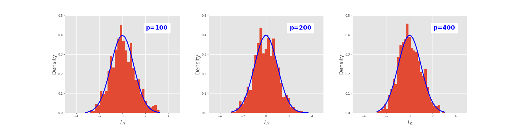
According to Theorem 4.2, $T_{n}$ weakly converges to the standard normal distribution as $n,p\rightarrow\infty.$ In this example, $c=2/3$ and $p=100,200,400.$ The finite-sample distribution of $T_{n}$ is presented by the histogram of $T_{n}$ in Figure 2 with 1000 repetitions, where the solid blue curve stands for standard normal density function. It can be seen that the finite-sample distribution of $T_{n}$ is very consistent with the standard normal distribution, especially when $n,p$ become larger. When $\alpha=0.05$ , the empirical cover rates of the $95\%$ -confidence interval are $93.1\%$ , $93.9\%$ and $95.2\%$ for $p=100$ , $200$ and $400$ respectively. All these experiments verify the correctness of our theoretical results.

Example 2. This example verifies the results in Theorem 4.5. Here we define two statistics:

	$\displaystyle T_{n,0}$	$\displaystyle=$	$\displaystyle\frac{\sqrt{p}}{\sigma_{c,3}}\Big\{R_{{\mathbf{X}}}(\hat{\bm{\beta}},{\bm{\beta}})-(1-\frac{1}{c_{n}})r^{2}-\frac{\sigma^{2}}{c_{n}-1}\Big\}-\frac{\mu_{c,3}}{\sigma_{c,3}},$
	$\displaystyle T_{n,1}$	$\displaystyle=$	$\displaystyle\frac{\sqrt{p}}{\tilde{\sigma}_{c,3}}\Big\{R_{{\mathbf{X}}}(\hat{\bm{\beta}},{\bm{\beta}})-(1-\frac{1}{c_{n}})r^{2}-\frac{\sigma^{2}}{c_{n}-1}\Big\}-\frac{\tilde{\mu}_{c,3}}{\tilde{\sigma}_{c,3}}.$

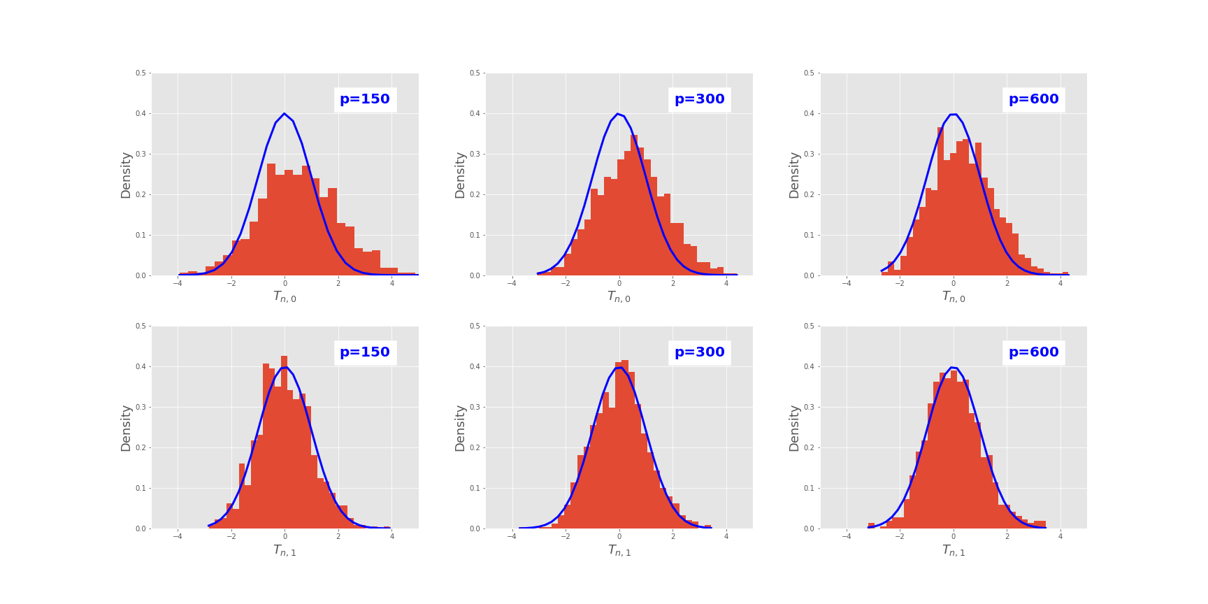
According to Theorem 4.5, both $T_{n,0}$ and $T_{n,1}$ weakly converge to the standard normal distribution as $n,p\rightarrow+\infty.$ We take $c=3/2$ and $p=150,300,450.$ Similarly the finite-sample distributions of $T_{n,0}$ and $T_{n,1}$ are presented by the histogram of $T_{n,0}$ and $T_{n,1}$ with 1000 repetitions. The comparison between these two statistics is shown in Figure 3. It can also be seen that the finite sample distributions of $T_{n,0}$ and $T_{n,1}$ both match the standard normal distribution quite well. The empirical cover rates of the $95\%$ -confidence interval (9) are $93.8\%$ , $94.7\%$ and $94.4\%$ for $p=150$ , $300$ and $600$ respectively, which further shows the validity of our theoretical results.

References

Advani & Saxe (2017) Madhu S Advani and Andrew M Saxe. High-dimensional dynamics of generalization error in neural networks. arXiv preprint arXiv:1710.03667, 2017.
Ba et al. (2019) Jimmy Ba, Murat Erdogdu, Taiji Suzuki, Denny Wu, and Tianzong Zhang. Generalization of two-layer neural networks: An asymptotic viewpoint. In International Conference on Learning Representations, 2019.
Bai & Silverstein (2004) Zhidong Bai and Jack W. Silverstein. Clt for linear spectral statistics of large-dimensional sample covariance matrices. The Annals of Probability, 32(1A):553–605, 2004.
Bai & Yao (2005) Zhidong Bai and Jianfeng Yao. On the convergence of the spectral empirical process of wigner matrices. Bernoulli, 11(6):1059–1092, 2005.
Bai & Yao (2008) Zhidong Bai and Jianfeng Yao. Central limit theorems for eigenvalues in a spiked population model. Annales de l’IHP Probabilités et statistiques, 44(3):447–474, 2008.
Bai & Yin (2008) Zhidong Bai and YongQua Yin. Limit of the smallest eigenvalue of a large dimensional sample covariance matrix. In Advances In Statistics, pp. 108–127. World Scientific, 2008.
Bai et al. (2007) Zhidong Bai, Baiqi Miao, and Guangming Pan. On asymptotics of eigenvectors of large sample covariance matrix. The Annals of Probability, 35(4):1532–1572, 2007.
Bartlett et al. (2020) Peter L Bartlett, Philip M Long, Gábor Lugosi, and Alexander Tsigler. Benign overfitting in linear regression. Proceedings of the National Academy of Sciences, 2020.
Belkin et al. (2018) Mikhail Belkin, Daniel Hsu, Siyuan Ma, and Soumik Mandal. Reconciling modern machine learning and the bias-variance trade-off. stat, 1050:28, 2018.
Belkin et al. (2019) Mikhail Belkin, Daniel Hsu, and Ji Xu. Two models of double descent for weak features. arXiv preprint arXiv:1903.07571, 2019.
Chen et al. (2020) Lin Chen, Yifei Min, Mingrui Zhang, and Amin Karbasi. More data can expand the generalization gap between adversarially robust and standard models. arXiv preprint arXiv:2002.04725, 2020.
Dar & Baraniuk (2020) Yehuda Dar and Richard G Baraniuk. Double double descent: On generalization errors in transfer learning between linear regression tasks. arXiv preprint arXiv:2006.07002, 2020.
Dar et al. (2020) Yehuda Dar, Paul Mayer, Lorenzo Luzi, and Richard G Baraniuk. Subspace fitting meets regression: The effects of supervision and orthonormality constraints on double descent of generalization errors. arXiv preprint arXiv:2002.10614, 2020.
Deng et al. (2019) Zeyu Deng, Abla Kammoun, and Christos Thrampoulidis. A model of double descent for high-dimensional binary linear classification. arXiv preprint arXiv:1911.05822, 2019.
Dereziński et al. (2019) Michał Dereziński, Feynman Liang, and Michael W Mahoney. Exact expressions for double descent and implicit regularization via surrogate random design. arXiv preprint arXiv:1912.04533, 2019.
Emami et al. (2020) Melikasadat Emami, Mojtaba Sahraee-Ardakan, Parthe Pandit, Sundeep Rangan, and Alyson K Fletcher. Generalization error of generalized linear models in high dimensions. arXiv preprint arXiv:2005.00180, 2020.
Geiger et al. (2019) Mario Geiger, Stefano Spigler, Stéphane d’Ascoli, Levent Sagun, Marco Baity-Jesi, Giulio Biroli, and Matthieu Wyart. Jamming transition as a paradigm to understand the loss landscape of deep neural networks. Physical Review E, 100(1):012115, 2019.
Gerbelot et al. (2020a) Cedric Gerbelot, Alia Abbara, and Florent Krzakala. Asymptotic errors for teacher-student convex generalized linear models (or: How to prove kabashima’s replica formula). arXiv preprint arXiv:2006.06581, 2020a.
Gerbelot et al. (2020b) Cédric Gerbelot, Alia Abbara, and Florent Krzakala. Asymptotic errors for convex penalized linear regression beyond gaussian matrices. arXiv preprint arXiv:2002.04372, 2020b.
Hastie et al. (2019) Trevor Hastie, Andrea Montanari, Saharon Rosset, and Ryan J Tibshirani. Surprises in high-dimensional ridgeless least squares interpolation. arXiv preprint arXiv:1903.08560, 2019.
Javanmard et al. (2020) Adel Javanmard, Mahdi Soltanolkotabi, and Hamed Hassani. Precise tradeoffs in adversarial training for linear regression. arXiv preprint arXiv:2002.10477, 2020.
Kini & Thrampoulidis (2020) Ganesh Kini and Christos Thrampoulidis. Analytic study of double descent in binary classification: The impact of loss. arXiv preprint arXiv:2001.11572, 2020.
LeJeune et al. (2020) Daniel LeJeune, Hamid Javadi, and Richard Baraniuk. The implicit regularization of ordinary least squares ensembles. In International Conference on Artificial Intelligence and Statistics, pp. 3525–3535, 2020.
Loog et al. (2019) Marco Loog, Tom Viering, and Alexander Mey. Minimizers of the empirical risk and risk monotonicity. In Advances in Neural Information Processing Systems, pp. 7478–7487, 2019.
Mei & Montanari (2019) Song Mei and Andrea Montanari. The generalization error of random features regression: Precise asymptotics and double descent curve. arXiv preprint arXiv:1908.05355, 2019.
Min et al. (2020) Yifei Min, Lin Chen, and Amin Karbasi. The curious case of adversarially robust models: More data can help, double descend, or hurt generalization. arXiv preprint arXiv:2002.11080, 2020.
Montanari et al. (2019) Andrea Montanari, Feng Ruan, Youngtak Sohn, and Jun Yan. The generalization error of max-margin linear classifiers: High-dimensional asymptotics in the overparametrized regime. arXiv preprint arXiv:1911.01544, 2019.
Muthukumar et al. (2020) Vidya Muthukumar, Kailas Vodrahalli, Vignesh Subramanian, and Anant Sahai. Harmless interpolation of noisy data in regression. IEEE Journal on Selected Areas in Information Theory, 2020.
Nakkiran (2019) Preetum Nakkiran. More data can hurt for linear regression: Sample-wise double descent. arXiv preprint arXiv:1912.07242, 2019.
Nakkiran et al. (2019) Preetum Nakkiran, Gal Kaplun, Yamini Bansal, Tristan Yang, Boaz Barak, and Ilya Sutskever. Deep double descent: Where bigger models and more data hurt. In International Conference on Learning Representations, 2019.
Pan & Zhou (2008) G. M. Pan and W. Zhou. Central limit theorem for signal-to-interference ratio of reduced rank linear receiver. Ann. Appl. Probab., 18(3):1232–1270, 06 2008. doi: 10.1214/07-AAP477. URL https://doi.org/10.1214/07-AAP477.
Sinai & Soshnikov (1998) Ya Sinai and Alexander Soshnikov. Central limit theorem for traces of large random symmetric matrices with independent matrix elements. Boletim da Sociedade Brasileira de Matemática-Bulletin/Brazilian Mathematical Society, 29(1):1–24, 1998.
Spigler et al. (2019) S Spigler, M Geiger, S d’Ascoli, L Sagun, G Biroli, and M Wyart. A jamming transition from under-to over-parametrization affects generalization in deep learning. Journal of Physics A: Mathematical and Theoretical, 52(47):474001, 2019.
Van der Vaart (2000) Aad W Van der Vaart. Asymptotic statistics, volume 3. Cambridge university press, 2000.
Xing et al. (2019) Yue Xing, Qifan Song, and Guang Cheng. Benefit of interpolation in nearest neighbor algorithms. arXiv preprint arXiv:1909.11720, 2019.
Xu & Hsu (2019) Ji Xu and Daniel J Hsu. On the number of variables to use in principal component regression. In Advances in Neural Information Processing Systems, pp. 5094–5103, 2019.
Zheng (2012) Shurong Zheng. Central limit theorems for linear spectral statistics of large dimensional f-matrices. Annales de l’IHP Probabilités et statistiques, 48(2):444–476, 2012.
Zheng et al. (2015) Shurong Zheng, Zhidong Bai, and Jianfeng Yao. Substitution principle for clt of linear spectral statistics of high-dimensional sample covariance matrices with applications to hypothesis testing. The Annals of Statistics, 43(2):546–591, 2015.

Appendix A Proof of theorem 4.1 and theorem 4.2

Let ${\mathbf{X}}={\mathbf{Z}}{\bm{\Sigma}}^{1/2}.$ According to the Bai-Yin theorem (Bai & Yin 2008), the smallest eigenvalue of ${\mathbf{Z}}^{\mathrm{\scriptscriptstyle T}}{\mathbf{Z}}/n$ is almost surely larger than $(1-\sqrt{c})^{2}/2$ for sufficiently large $n.$ Thus

\lambda_{min}(\frac{1}{n}{\mathbf{X}}^{\mathrm{\scriptscriptstyle T}}{\mathbf{X}})\geq c_{0}\lambda_{\min}(\frac{1}{n}{\mathbf{Z}}^{\mathrm{\scriptscriptstyle T}}{\mathbf{Z}})\geq\frac{c_{0}}{2}(1-\sqrt{c})^{2},

which implies that the matrix ${\mathbf{X}}^{\mathrm{\scriptscriptstyle T}}{\mathbf{X}}/n$ is almost surely invertible for large $n.$ By Section 3.2, ${\bm{\Pi}}={\bf 0}$ , $B_{\mathbf{X}}(\hat{\bm{\beta}},{\bm{\beta}})=B_{{\mathbf{X}},{\bm{\beta}}}(\hat{\bm{\beta}},{\bm{\beta}})=0$ and $V_{\mathbf{X}}(\hat{\bm{\beta}},{\bm{\beta}})=V_{{\mathbf{X}},{\bm{\beta}}}(\hat{\bm{\beta}},{\bm{\beta}}).$ Thus the CLT of $R_{\mathbf{X}}(\hat{\bm{\beta}},{\bm{\beta}})$ is same to that of $R_{{\mathbf{X}},{\bm{\beta}}}(\hat{\bm{\beta}},{\bm{\beta}}).$ For simplicity, we focus on $R_{\mathbf{X}}(\hat{\bm{\beta}},{\bm{\beta}})$ in the following. Notice that

$\displaystyle V_{\mathbf{X}}(\hat{\bm{\beta}},{\bm{\beta}})$	$\displaystyle=$	$\displaystyle\frac{\sigma^{2}}{n}\Tr(\hat{{\bm{\Sigma}}}^{-1}{\bm{\Sigma}})$
	$\displaystyle=$	$\displaystyle\frac{\sigma^{2}}{n}\Tr\Big({\bm{\Sigma}}^{-1/2}\big(\frac{{\mathbf{Z}}^{\mathrm{\scriptscriptstyle T}}{\mathbf{Z}}}{n}\big)^{-1}{\bm{\Sigma}}^{-1/2}{\bm{\Sigma}}\Big)$
	$\displaystyle=$	$\displaystyle\frac{\sigma^{2}}{n}\sum_{i=1}^{p}\frac{1}{s_{i}}=\frac{\sigma^{2}p}{n}\int\frac{1}{s}dF_{{\mathbf{Z}}}(s)$

where $F_{{\mathbf{Z}}}$ is the spectral measure of ${\mathbf{Z}}^{\mathrm{\scriptscriptstyle T}}{\mathbf{Z}}/n.$ According to Theorem 1 of Hastie et al. 2019, as $n,p\rightarrow\infty$ such that $p/n=c_{n}\rightarrow c\in(0,\infty)$ , $F_{\mathbf{Z}}(x)$ weakly converges to the standard Marcenko-Pastur law $F_{c}(x)$ and

\displaystyle V_{\mathbf{X}}(\hat{\bm{\beta}},{\bm{\beta}})\rightarrow\sigma^{2}c\int\frac{1}{s}dF_{c}(s)=\sigma^{2}\frac{c}{1-c}.

Here the standard Marcenko-Pastur law $F_{c}(x)$ has a density function

p_{c}(x)=\left\{\begin{array}[]{ll}\frac{1}{2\pi cx}\sqrt{(b-x)(x-a)},&\mbox{ if }a\leq x\leq b,\\ 0,&\mbox{o.w.},\end{array}\right.

where $a=(1-\sqrt{c})^{2}$ , $b=(1+\sqrt{c})^{2}$ and $p_{c}(x)$ has a point mass $1-\frac{1}{c}$ at the origin if $c>1$ . Hence

	$\displaystyle R_{\mathbf{X}}(\hat{\bm{\beta}},{\bm{\beta}})-\sigma^{2}\frac{c_{n}}{1-c_{n}}$	$\displaystyle=$	$\displaystyle\frac{\sigma^{2}p}{n}\int\frac{1}{s}dF_{Z}(s)-\sigma^{2}c_{n}\int\frac{1}{s}dF_{c_{n}}(s)$
		$\displaystyle=$	$\displaystyle\sigma^{2}c_{n}\int\frac{1}{s}\big(dF_{Z}(s)-dF_{c_{n}}(s)\big).$

According to Theorem 1.1 of Bai & Silverstein 2004,

p\Big(R_{\mathbf{X}}(\hat{\bm{\beta}},{\bm{\beta}})-\sigma^{2}\frac{c_{n}}{1-c_{n}}\Big)\xrightarrow{d}N(\mu_{c},\sigma^{2}_{c}),

(10)

where

$\displaystyle\mu_{c}$	$\displaystyle=$	$\displaystyle-\frac{\sigma^{2}c}{2\pi i}\oint_{\gamma}\frac{1}{z}\frac{c\underline{m}(z)^{3}(1+\underline{m}(z))^{-3}}{\left\{1-c\underline{m}(z)^{2}(1+\underline{m}(z))^{-2}\right\}^{2}}dz$	(11)
		$\displaystyle-\frac{\sigma^{2}c(\nu_{4}-3)}{2\pi i}\oint_{\gamma}\frac{1}{z}\frac{c\underline{m}(z)^{3}(1+\underline{m}(z))^{-3}}{1-c\underline{m}(z)^{2}(1+\underline{m}(z))^{-2}}dz,$	(11)
$\displaystyle\sigma^{2}_{c}$	$\displaystyle=$	$\displaystyle-\frac{\sigma^{4}c^{2}}{2\pi^{2}}\oint_{{\color[rgb]{1,0,0}\mathcal{C}_{1}}}\oint_{{\color[rgb]{1,0,0}\mathcal{C}_{2}}}\frac{1}{z_{1}z_{2}}\frac{1}{(\underline{m}(z_{1})-\underline{m}(z_{2}))^{2}}\frac{d}{dz_{1}}\underline{m}(z_{1})\frac{d}{dz_{2}}\underline{m}(z_{2})dz_{1}dz_{2}$	(12)
		$\displaystyle-\frac{\sigma^{4}c^{3}(\nu_{4}-3)}{4\pi^{2}}\oint_{{\color[rgb]{1,0,0}\mathcal{C}_{1}}}\oint_{{\color[rgb]{1,0,0}\mathcal{C}_{2}}}\frac{1}{z_{1}z_{2}}\frac{1}{(1+\underline{m}(z_{1}))^{2}(1+\underline{m}(z_{2}))^{2}}d\underline{m}(z_{1})d\underline{m}(z_{2}).$	(12)

Here the contours in (11) and (12) are closed and taken in the positive direction in the complex plane, enclosing the support of $F_{\mathbf{Z}}$ , i.e. $[(1-\sqrt{c})^{2},(1+\sqrt{c})^{2}]$ . The Stieltjes transform $\underline{m}(z)$ satisfies the equation

z=-\frac{1}{\underline{m}}+\frac{c}{1+\underline{m}}.

To further simplify the integrations in $\mu_{c}$ and $\sigma_{c}$ , let $z=1+\sqrt{c}(r\xi+\frac{1}{r\xi})+c$ and perform change of variables, then we have

\underline{m}(z)=-\frac{1}{1+\sqrt{c}r\xi},\quad dz=\sqrt{c}(r-\frac{1}{r\xi^{2}})d\xi,\quad d\underline{m}=\frac{\sqrt{c}r}{(1+\sqrt{c}r\xi)^{2}}d\xi

and when $\xi$ moves along the unit circle $|\xi|=1$ on the complex plane, $z$ will orbit around the center point $1+c$ along an ellipse which enclosing the support of $F_{\mathbf{Z}}$ . Thus

$\displaystyle\mu_{c}$	$\displaystyle=$	$\displaystyle-\frac{\sigma^{2}c}{2\pi i}\oint_{\gamma}\frac{1}{z}\frac{c\underline{m}(z)^{3}(1+\underline{m}(z))^{-3}}{(1-c\underline{m}(z)^{2}(1+\underline{m}(z))^{-2})^{2}}dz$
		$\displaystyle-\frac{\sigma^{2}c(\nu_{4}-3)}{2\pi i}\oint_{\gamma}\frac{1}{z}\frac{c\underline{m}(z)^{3}(1+\underline{m}(z))^{-3}}{1-c\underline{m}(z)^{2}(1+\underline{m}(z))^{-2}}dz$
	$\displaystyle=$	$\displaystyle\frac{\sigma^{2}c}{2\pi i}\oint_{\|\xi\|=1}\frac{1}{r(\sqrt{c}+r\xi)(1+\sqrt{c}r\xi)(\xi-\frac{1}{r})(\xi+\frac{1}{r})}d\xi$
		$\displaystyle+\frac{\sigma^{2}c(\nu_{4}-3)}{2\pi i}\oint_{\|\xi\|=1}\frac{1}{r\xi^{2}(\sqrt{c}+r\xi)(1+\sqrt{c}r\xi)}d\xi$
	$\displaystyle=$	$\displaystyle\frac{\sigma^{2}c^{2}}{(c-1)^{2}}+\frac{\sigma^{2}c^{2}(\nu_{4}-3)}{1-c}.$

As for $\sigma_{c}^{2}$ , note that

			$\displaystyle\frac{1}{2\pi i}\oint_{\gamma_{1}}\frac{1}{z_{1}(\underline{m}_{1}-\underline{m}_{2})^{2}}d\underline{m}_{1}$
		$\displaystyle=$	$\displaystyle\frac{1}{2\pi i}\oint_{\|\xi_{1}\|=1}\frac{1}{1+\sqrt{c}(r_{1}\xi_{1}+\frac{1}{r_{1}\xi_{1}})+c}\cdot\frac{\sqrt{c}~r_{1}}{(\underline{m}_{2}+\frac{1}{1+\sqrt{c}r_{1}\xi_{1}})^{2}(1+\sqrt{c}r_{1}\xi_{1})^{2}}d\xi_{1}$
		$\displaystyle=$	$\displaystyle\frac{1}{2\pi i}\oint_{\|\xi_{1}\|=1}\frac{\sqrt{c}~r_{1}\xi_{1}}{(\xi_{1}+\frac{\sqrt{c}}{r_{1}})(r_{1}\xi_{1}\sqrt{c}+1)\left\{(r_{1}\xi_{1}\sqrt{c}+1)\underline{m}_{2}+1\right\}^{2}}d\xi_{1}$
		$\displaystyle=$	$\displaystyle\frac{c}{(c-1)\left\{(c-1)\underline{m}_{2}-1\right\}^{2}},$

therefore

			$\displaystyle-\frac{\sigma^{4}c^{2}}{2\pi^{2}}\oiint\frac{1}{z_{1}z_{2}(\underline{m}_{1}-\underline{m}_{2})^{2}}d\underline{m_{1}}d\underline{m}_{2}$
		$\displaystyle=$	$\displaystyle\frac{2\sigma^{4}c^{2}}{2\pi i}\oint_{\|\xi_{2}\|=1}\frac{c}{z_{2}(c-1)\left\{(c-1)\underline{m}_{2}-1\right\}^{2}}d\underline{m_{2}}$
		$\displaystyle=$	$\displaystyle\frac{2\sigma^{4}c^{2}}{2\pi i}\oint_{\|\xi_{2}\|=1}\frac{\sqrt{c}~r_{2}^{2}\xi_{2}}{(c-1)(1+\sqrt{c}~r_{2}\xi_{2})(\sqrt{c}+r_{2}\xi_{2})^{3}}d\xi_{2}=\frac{2c^{3}\sigma^{4}}{(c-1)^{4}}.$

Meanwhile,

			$\displaystyle\frac{1}{2\pi i}\oint_{\gamma_{1}}\frac{1}{z_{1}}\frac{1}{(1+\underline{m}(z_{1}))^{2}}d\underline{m}(z_{1})$
		$\displaystyle=$	$\displaystyle\frac{1}{2\pi i}\oint_{\|\xi\|=1}\frac{1}{\sqrt{c}\xi(1+\sqrt{c}r\xi)(\sqrt{c}+r\xi)}d\xi=\frac{1}{c-1},$

hence

-\frac{\sigma^{4}c^{3}(\nu_{4}-3)}{4\pi^{2}}\oint_{\mathcal{C}_{1}}\oint_{\mathcal{C}_{2}}\frac{1}{z_{1}z_{2}}\frac{1}{(1+\underline{m}(z_{1}))^{2}(1+\underline{m}(z_{2}))^{2}}d\underline{m}(z_{1})d\underline{m}(z_{2})=\frac{\sigma^{4}c^{3}(\nu_{4}-3)}{(1-c)^{2}},

and

\sigma_{c}^{2}=\frac{2c^{3}\sigma^{4}}{(c-1)^{4}}+\frac{\sigma^{4}c^{3}(\nu_{4}-3)}{(1-c)^{2}}.

Let

T_{n}=\frac{p}{\sigma_{c}}\Big(R_{\mathbf{X}}(\hat{\bm{\beta}},{\bm{\beta}})-\sigma^{2}\frac{c_{n}}{1-c_{n}}-\frac{\mu_{c}}{p}\Big).

According to (10), we have

P(L_{\alpha,c}\leq R_{{\mathbf{X}},{\bm{\beta}}}(\hat{\bm{\beta}},{\bm{\beta}})\leq U_{\alpha,c})=P(-Z_{\alpha/2}\leq T_{n}\leq Z_{\alpha/2})\rightarrow 1-\alpha,

where

	$\displaystyle L_{\alpha,c}$	$\displaystyle=$	$\displaystyle\sigma^{2}\frac{c_{n}}{1-c_{n}}+\frac{1}{p}(\mu_{c}-Z_{\alpha/2}\sigma_{c}),$
	$\displaystyle U_{\alpha,c}$	$\displaystyle=$	$\displaystyle\sigma^{2}\frac{c_{n}}{1-c_{n}}+\frac{1}{p}(\mu_{c}+Z_{\alpha/2}\sigma_{c}).$

$\Box$

Appendix B Proof of theorem 4.3

Notice that

$\displaystyle B_{\mathbf{X}}(\hat{\bm{\beta}},{\bm{\beta}})$	$\displaystyle=$	$\displaystyle{\bm{\beta}}^{\mathrm{\scriptscriptstyle T}}({\bm{I}}_{p}-\hat{{\bm{\Sigma}}}^{+}\hat{{\bm{\Sigma}}}){\bm{\beta}}$
	$\displaystyle=$	$\displaystyle\lim_{z\rightarrow 0^{+}}{\bm{\beta}}^{\mathrm{\scriptscriptstyle T}}\big({\bm{I}}_{p}-(\hat{\bm{\Sigma}}+z{\bm{I}}_{p})^{-1}\hat{\bm{\Sigma}}\big){\bm{\beta}}$
	$\displaystyle=$	$\displaystyle\lim_{z\rightarrow 0^{+}}z{\bm{\beta}}^{\mathrm{\scriptscriptstyle T}}(\hat{\bm{\Sigma}}+z{\bm{I}}_{p})^{-1}{\bm{\beta}}.$

Since ${\bm{\beta}}$ is a constant vector, we can make use of the results in Theorem 3 in Bai et al. 2007 and Theorem 1.3 in Pan & Zhou 2008 regarding eigenvectors. Their works investigate the sample covariance matrix ${\mathbf{A}}_{p}={\bm{T}}_{p}^{1/2}{\mathbf{X}}_{p}^{\mathrm{\scriptscriptstyle T}}{\mathbf{X}}_{p}{\bm{T}}_{p}^{1/2}/n$ , where ${\bm{T}}_{p}$ is an $p\times p$ nonnegative definite Hermitian matrix with a square root ${\bm{T}}_{p}^{1/2}$ and ${\mathbf{X}}_{p}$ is an $n\times p$ matrix with i.i.d. entries $({\textnormal{x}}_{ij})_{n\times p}$ . Let ${\bm{U}}_{p}{\bm{\Lambda}}_{p}{\bm{U}}_{p}^{\mathrm{\scriptscriptstyle T}}$ denote the spectral decomposition of ${\mathbf{A}}_{p}$ where ${\bm{\Lambda}}_{p}=\mbox{diag}(\lambda_{1},\cdots,\lambda_{p})$ and ${\bm{U}}_{p}$ is a unitary matrix consisting of the orthonormal eigenvectors of ${\mathbf{A}}_{p}$ . Assume that ${\bm{x}}_{p}$ is an arbitrary nonrandom unit vector and ${\bm{y}}=(y_{1},y_{2},\cdots,y_{p})^{\mathrm{\scriptscriptstyle T}}={\bm{U}}_{p}^{\mathrm{\scriptscriptstyle T}}{\bm{x}}_{p}$ , two empirical distribution functions based on eigenvectors and eigenvalues are defined as

F_{1}^{{\mathbf{A}}_{p}}(x)=\sum_{i=1}^{p}|y_{i}|^{2}\mathds{1}(\lambda_{i}\leq x),\quad F^{{\mathbf{A}}_{p}}(x)=\frac{1}{p}\sum_{i=1}^{p}\mathds{1}(\lambda_{i}\leq x).

Then for a bounded continuous function $g(x)$ , we have

\sum_{j=1}^{p}|{\textnormal{y}}_{j}|^{2}g(\lambda_{j})-\frac{1}{p}\sum_{j=1}^{p}g(\lambda_{j})=\int g(x)dF_{1}^{{\bm{A}}_{p}}(x)-\int g(x)dF^{{\bm{A}}_{p}}(x).

The results in Bai et al. 2007 and Pan & Zhou 2008 show that

Lemma B.1.

(Theorem 3 Bai et al. 2007 and Theorem 1.3 Pan & Zhou 2008) Suppose that

(1)

${\textnormal{x}}_{ij}$ ’s are i.i.d. satisfying $\mathbb{E}({\textnormal{x}}_{ij})=0$ , $\mathbb{E}(|{\textnormal{x}}_{ij}|^{2})=1$ and $\mathbb{E}(|{\textnormal{x}}_{ij}|^{4})<\infty$ ;
(2)

${\bm{x}}_{p}\in{\mathbb{C}}^{p}$ , $\|{\bm{x}}_{p}\|=1$ , $\lim_{n,p\rightarrow\infty}p/n=c\in(0,\infty)$ ;
(3)

${\bm{T}}_{p}$ is nonrandom Hermitian non-negative definite with with its spectral norm bounded in $p$ , with $H_{p}=F^{{\bm{T}}_{p}}\xrightarrow{d}H$ a proper distribution function and ${\bm{x}}_{p}^{\mathrm{\scriptscriptstyle T}}({\bm{T}}_{p}-z{\bm{I}}_{p})^{-1}{\bm{x}}_{p}\rightarrow m_{F^{H}}(z)$ , where $m_{F^{H}}(z)$ denotes the Stieltjes transform of $H(t)$ ;

(4)

$g_{1},\cdots,g_{k}$ are analytic functions on an open region of the complex plain which contains the real interval

\Big[\liminf_{p}\lambda_{min}({\bm{T}}_{p})\mathds{1}_{(0,1)}(c)(1-\sqrt{c})^{2},\,\,\limsup_{p}\lambda_{max}({\bm{T}}_{p})\mathds{1}_{(0,1)}(c)(1+\sqrt{c})^{2}\Big];

(5)

as $n,p\rightarrow\infty$ ,

\sup_{z}\sqrt{n}\Big\|{\bm{x}}_{p}^{\mathrm{\scriptscriptstyle T}}\big(\underline{m}_{F^{c_{n},H_{p}}}(z){\bm{T}}_{p}-{\bm{I}}_{p}\big)^{-1}{\bm{x}}_{p}-\int\frac{1}{1+t\underline{m}_{F^{c_{n},H_{p}}}(z)}dH_{n}(t)\Big\|\rightarrow 0.

Define $G_{p}(x)=\sqrt{n}(F_{1}^{{\bm{A}}_{p}}(x)-F^{{\bm{A}}_{p}}(x))$ , then the random vectors

\left(\int g_{1}(x)dG_{p}(x),\cdots,\int g_{k}(x)dG_{p}(x)\right)

forms a tight sequence and converges weakly to a Gaussian vector ${\textnormal{x}}_{g_{1}},\cdots,{\textnormal{x}}_{g_{k}}$ with mean zero and covariance function

\mathrm{Cov}({\textnormal{x}}_{g_{1}},{\textnormal{x}}_{g_{2}})=-\frac{1}{2\pi^{2}}\int_{{\mathbb{C}}_{1}}\int_{{\mathbb{C}}_{2}}g_{1}(z_{1})g_{2}(z_{2})\frac{(z_{2}\underline{m}_{2}-z_{1}\underline{m}_{1})^{2}}{c^{2}z_{1}z_{2}(z_{2}-z_{1})(\underline{m}_{2}-\underline{m}_{1})}dz_{1}dz_{2}.

The contours ${\mathbb{C}}_{1}$ , ${\mathbb{C}}_{2}$ are disjoint, both contained in the analytic region for the functions $(g_{1},\cdots,g_{k})$ and enclose the support of $F^{c_{n},H_{p}}$ for all large $p$ .

(6)

If $H(x)$ satisfies

\int\frac{dH(t)}{(1+t\underline{m}(z_{1}))(1+t\underline{m}(z_{2}))}=\int\frac{dH(t)}{1+t\underline{m}(z_{1})}\int\frac{dH(t)}{1+t\underline{m}(z_{2})},

then the covariance function can be further simplified to

\mathrm{Cov}({\textnormal{x}}_{g_{1}},{\textnormal{x}}_{g_{2}})=\frac{2}{c}(\int g_{1}(x)g_{2}(x)dF^{c,H}(x)-\int g_{1}(x)dF^{c,H}(x)\int g_{2}(x)dF^{c,H}(x)).

Recall that $B_{\mathbf{X}}(\hat{\bm{\beta}},{\bm{\beta}})=\lim_{z\rightarrow 0^{+}}z{\bm{\beta}}^{\mathrm{\scriptscriptstyle T}}(\hat{\bm{\Sigma}}+z{\bm{I}}_{p})^{-1}{\bm{\beta}}$ . Let $g(x)=1/(x+z)$ and ${\bm{x}}_{p}={\bm{\beta}}/r$ . Then we have

\int g(x)dG_{n}(x)=\sqrt{n}\Big(\frac{1}{r^{2}}{\bm{\beta}}^{\mathrm{\scriptscriptstyle T}}(\hat{\bm{\Sigma}}+z{\bm{I}}_{p})^{-1}{\bm{\beta}}-\int g(x)dF_{c_{n}}(x)\Big),

where $F_{c_{n}}(x)$ is the standard Marcenko-Pastur law. It is not difficult to check that under Assumptions (A1), (B1) and (C1), all the conditions (1)-(6) in Lemma B.1 are satisfied.

To proceed further, denote $a=(1-\sqrt{c})^{2}$ , $b=(1+\sqrt{c})^{2}$ . If $c$ is replaced by $c_{n}$ , $a$ and $b$ are denoted by $a_{n}$ and $b_{n}$ respectively. By some algebraic calculations, we have

	$\displaystyle\int g(x)dF_{c_{n}}(x)$	$\displaystyle=$	$\displaystyle(1-\frac{1}{c_{n}})\cdot\frac{1}{z}+\int_{a_{n}}^{b_{n}}\frac{1}{x+z}\cdot\frac{1}{2\pi c_{n}x}\sqrt{(b_{n}-x)(x-a_{n})}dx$
		$\displaystyle=$	$\displaystyle(1-\frac{1}{c_{n}})\cdot\frac{1}{z}-\frac{-1+c_{n}+z-\sqrt{c_{n}^{2}+2c_{n}(z-1)+(1+z)^{2}}}{2c_{n}z},$

and

$\displaystyle\mathrm{Var}({\textnormal{x}}_{g})$	$\displaystyle=$	$\displaystyle\frac{2}{c}\left(\int\{g(x)\}^{2}dF_{c}(x)-\big\{\int g(x)dF_{c}(x)\big\}^{2}\right)$
	$\displaystyle=$	$\displaystyle\frac{2}{c}\Big((1-\frac{1}{c})\cdot\frac{1}{z^{2}}+\int_{a}^{b}\frac{1}{(x+z)^{2}}\cdot\frac{1}{2\pi cx}\sqrt{(b-x)(x-a)}dx\Big)$
		$\displaystyle-\frac{2}{c}\Big((1-\frac{1}{c})\cdot\frac{1}{z}+\int_{a}^{b}\frac{1}{x+z}\cdot\frac{1}{2\pi cx}\sqrt{(b-x)(x-a)}dx\Big)^{2}.$

Therefore,

\lim_{z\rightarrow 0^{+}}z\int g(x)dF_{c_{n}}(x)=1-\frac{1}{c_{n}}\quad\text{and}\quad\lim_{z\rightarrow 0^{+}}z^{2}\mathrm{Var}({\textnormal{x}}_{g})=\frac{2(c-1)}{c^{3}}.

Furthermore, as $n,p\rightarrow\infty$ , $p/n=c_{n}\rightarrow c>1$ ,

\sqrt{n}\Big(B_{\mathbf{X}}(\hat{\bm{\beta}},{\bm{\beta}})-(1-\frac{1}{c_{n}})r^{2}\Big)\xrightarrow{d}N\Big(0,\frac{2(c-1)}{c^{3}}r^{4}\Big).

This can be rewritten as

\sqrt{p}\Big(B_{\mathbf{X}}(\hat{\bm{\beta}},{\bm{\beta}})-(1-\frac{1}{c_{n}})r^{2}\Big)\xrightarrow{d}N\Big(0,\frac{2(c-1)}{c^{2}}r^{4}\Big).

Next we deal with the variance term $V_{{\mathbf{X}}}(\hat{\bm{\beta}},{\bm{\beta}})$ . According to the Assumption (B1), the variance term is

\displaystyle V_{\mathbf{X}}(\hat{\bm{\beta}},{\bm{\beta}})=\frac{\sigma^{2}}{n}\Tr\{\hat{\bm{\Sigma}}^{+}\}=\frac{\sigma^{2}}{n}\sum_{i=1}^{n}\frac{1}{s_{i}},

where $s_{i}$ , $i=1,\dots,n$ are the nonzero eigenvalues of ${\mathbf{X}}^{\mathrm{\scriptscriptstyle T}}{\mathbf{X}}/n.$ Let $\{t_{i},~i=1,\ldots n\}$ denote the non-zero eigenvalues of ${\mathbf{X}}{\mathbf{X}}^{\mathrm{\scriptscriptstyle T}}/p$ , then we have

\displaystyle V_{\mathbf{X}}(\hat{\bm{\beta}},{\bm{\beta}})=\frac{\sigma^{2}}{p}\sum_{i=1}^{n}\frac{1}{t_{i}}=\frac{\sigma^{2}n}{p}\int\frac{1}{t}dF_{{\mathbf{X}}{\mathbf{X}}^{\mathrm{\scriptscriptstyle T}}/p}(t)\rightarrow\frac{\sigma^{2}}{c-1}.

By interchanging the role of $p$ and $n$ , from the result in Theorem 4.1, as $n,p\rightarrow\infty$ , $p/n=c_{n}\rightarrow c>1$ , we have,

\sum_{i=1}^{n}\frac{1}{t_{i}}-\frac{n}{1-c^{\prime}_{n}}\xrightarrow{d}N\Big(\frac{c^{\prime}}{(c^{\prime}-1)^{2}}+\frac{c^{\prime}(\nu_{4}-3)}{1-c^{\prime}},~\frac{2c^{\prime}}{(c^{\prime}-1)^{4}}+\frac{c^{\prime}(\nu_{4}-3)}{(1-c^{\prime})^{2}}\Big).

where $c^{\prime}_{n}=n/p=1/c_{n}$ , $c^{\prime}=1/c$ . This result can be rewritten as

\sum_{i=1}^{n}\frac{1}{t_{i}}-\frac{p}{c_{n}-1}\xrightarrow{d}N\Big(\frac{c}{(1-c)^{2}}+\frac{(\nu_{4}-3)}{c-1},~\frac{2c^{3}}{(1-c)^{4}}+\frac{c(\nu_{4}-3)}{(c-1)^{2}}\Big).

Hence the CLT of $V_{{\mathbf{X}}}(\hat{\bm{\beta}},{\bm{\beta}})$ is given by

p\Big(V_{\mathbf{X}}(\hat{\bm{\beta}},{\bm{\beta}})-\frac{\sigma^{2}}{c_{n}-1}\Big)\xrightarrow{d}N\Big(\frac{c\sigma^{2}}{(1-c)^{2}}+\frac{\sigma^{2}(\nu_{4}-3)}{c-1},~\frac{2c^{3}\sigma^{4}}{(1-c)^{4}}+\frac{c\sigma^{4}(\nu_{4}-3)}{(c-1)^{2}}\Big).

Notice that $\mathrm{Cov}\Big(B_{{\mathbf{X}}}(\hat{\bm{\beta}},{\bm{\beta}}),~V_{{\mathbf{X}}}(\hat{\bm{\beta}},{\bm{\beta}})\Big)=0.$ According to the consistency rate and the limiting distribution of $B_{{\mathbf{X}}}(\hat{\bm{\beta}},{\bm{\beta}})$ and $V_{{\mathbf{X}}}(\hat{\bm{\beta}},{\bm{\beta}})$ , we know that the bias $B_{{\mathbf{X}}}(\hat{\bm{\beta}},{\bm{\beta}})$ is the leading term of $R_{{\mathbf{X}}}(\hat{\bm{\beta}},{\bm{\beta}})$ . This implies that

\sqrt{p}\Big\{R_{{\mathbf{X}}}(\hat{\bm{\beta}},{\bm{\beta}})-(1-\frac{1}{c_{n}})\|{\bm{\beta}}\|_{2}^{2}-\frac{\sigma^{2}}{c_{n}-1}\Big\}\xrightarrow{d}N\big(0,\sigma_{c,1}^{2}\big),

where $\sigma_{c,1}^{2}=2(c-1)r^{4}/c^{2}.$ A practical version of this CLT is given by

\sqrt{p}\Big\{R_{{\mathbf{X}}}(\hat{\bm{\beta}},{\bm{\beta}})-(1-\frac{1}{c_{n}})\|{\bm{\beta}}\|_{2}^{2}-\frac{\sigma^{2}}{c_{n}-1}\Big\}\xrightarrow{d}N\big(\tilde{\mu}_{c,1},\tilde{\sigma}_{c,1}^{2}\big),

where

	$\displaystyle\tilde{\mu}_{c,1}$	$\displaystyle=$	$\displaystyle\frac{1}{\sqrt{p}}\Big\{\frac{c\sigma^{2}}{(1-c)^{2}}+\frac{\sigma^{2}(\nu_{4}-3)}{c-1}\Big\},$
	$\displaystyle\tilde{\sigma}_{c,1}^{2}$	$\displaystyle=$	$\displaystyle\frac{2(c-1)}{c^{2}}r^{4}+\frac{1}{p}\Big\{\frac{2c^{3}\sigma^{4}}{(1-c)^{4}}+\frac{c\sigma^{4}(\nu_{4}-3)}{(c-1)^{2}}\Big\}.$

Appendix C Proof of theorem 4.4

First we consider the bias term $B_{\mathbf{X}}(\hat{\bm{\beta}},{\bm{\beta}})$ . By Assumption (A1), (B1), and (C2),

$\displaystyle B_{\mathbf{X}}(\hat{\bm{\beta}},{\bm{\beta}})$	$\displaystyle=$	$\displaystyle\mathbb{E}[{\bm{\beta}}^{\mathrm{\scriptscriptstyle T}}\Pi{\bm{\Sigma}}\Pi{\bm{\beta}}\|{\mathbf{X}}]=\mathbb{E}[{\bm{\beta}}^{\mathrm{\scriptscriptstyle T}}\Pi{\bm{\beta}}\|{\mathbf{X}}]$
	$\displaystyle=$	$\displaystyle\Tr\left\{({\bm{I}}_{p}-\hat{\bm{\Sigma}}^{+}\hat{\bm{\Sigma}})\mathbb{E}({\bm{\beta}}{\bm{\beta}}^{\mathrm{\scriptscriptstyle T}}\|{\mathbf{X}})\right\}$
	$\displaystyle=$	$\displaystyle\frac{r^{2}}{p}\Tr\{{\bm{I}}_{p}-{\hat{\bm{\Sigma}}}^{+}{\hat{\bm{\Sigma}}}\}=r^{2}(1-n/p).$

Alternatively, we can rewrite the bias as

$\displaystyle B_{\mathbf{X}}(\hat{\bm{\beta}},{\bm{\beta}})$	$\displaystyle=$	$\displaystyle\lim_{z\rightarrow 0^{+}}\mathbb{E}[{\bm{\beta}}^{\mathrm{\scriptscriptstyle T}}({\bm{I}}_{p}-(\hat{\bm{\Sigma}}+z{\bm{I}}_{p})^{-1}\hat{\bm{\Sigma}}\big){\bm{\beta}}\|{\mathbf{X}}]$
	$\displaystyle=$	$\displaystyle\lim_{z\rightarrow 0^{+}}\mathbb{E}[z{\bm{\beta}}^{\mathrm{\scriptscriptstyle T}}(\hat{\bm{\Sigma}}+z{\bm{I}}_{p})^{-1}{\bm{\beta}}\|{\mathbf{X}}]$
	$\displaystyle=$	$\displaystyle\lim_{z\rightarrow 0^{+}}z\frac{r^{2}}{p}\Tr(\hat{\bm{\Sigma}}+z{\bm{I}}_{p})^{-1}.$

Define that $f_{n}(z)=z\frac{r^{2}}{p}\Tr(\hat{\bm{\Sigma}}+z{\bm{I}}_{p})^{-1}.$ Notice that $|f_{n}(z)|$ and $|f^{\prime}_{n}(z)|$ are bounded above. By the Arzela-Ascoli theorem, we deduce that $f_{n}(z)$ converges uniformly to its limit. Under Assumption (C2), by the Moore-Osgood theorem, almost surely,

	$\displaystyle\lim_{n,p\rightarrow\infty}B_{\mathbf{X}}(\hat{\bm{\beta}},{\bm{\beta}})$	$\displaystyle=$	$\displaystyle\lim_{z\rightarrow 0^{+}}\lim_{n,p\rightarrow\infty}z\frac{r^{2}}{p}\Tr(\hat{\bm{\Sigma}}+z{\bm{I}}_{p})^{-1}$
		$\displaystyle=$	$\displaystyle\lim_{z\rightarrow 0^{+}}\lim_{n,p\rightarrow\infty}z\frac{r^{2}}{p}\Tr\left(\frac{1}{n}{\mathbf{X}}{\mathbf{X}}^{{\mathrm{\scriptscriptstyle T}}}+z{\bm{I}}_{n}\right)^{-1},$

In fact,

\lim_{n,p\rightarrow\infty}B_{\mathbf{X}}(\hat{\bm{\beta}},{\bm{\beta}})=r^{2}\lim_{z\rightarrow 0^{+}}\lim_{n,p\rightarrow\infty}zm_{n}(-z),

where $m_{n}(z)$ is the Stieltjes transform of empirical spectral distribution of $\hat{\bm{\Sigma}}={\mathbf{X}}^{{\mathrm{\scriptscriptstyle T}}}{\mathbf{X}}/n.$ According to Theorem 2.1 in Zheng et al. 2015 and Lemma 1.1 in Bai & Silverstein 2004, the truncated version of $p(m_{n}(z)-m(z))$ converges weakly to a two-dimensional Gaussian process $M(\cdot)$ satisfying

\displaystyle\mathbb{E}[M(z)]

\displaystyle=

\displaystyle\frac{c\underline{m}^{3}(1+\underline{m})}{\left\{(1+\underline{m})^{2}-c\underline{m}^{2}\right\}^{2}}+\frac{c(\nu_{4}-3)\underline{m}^{3}}{(1+\underline{m})\left\{(1+\underline{m})^{2}-c\underline{m}^{2}\right\}},

and

	$\displaystyle\mathrm{Cov}\big(M(z_{1}),M(z_{2})\big)$	$\displaystyle=$	$\displaystyle 2\Big\{\frac{\underline{m}^{\prime}(z_{1})\underline{m}^{\prime}(z_{2})}{(\underline{m}(z_{1})-\underline{m}(z_{2}))^{2}}-\frac{1}{(z_{1}-z_{2})^{2}}\Big\}$
			$\displaystyle+\frac{c(\nu_{4}-3)\underline{m}^{\prime}(z_{1})\underline{m}^{\prime}(z_{2})}{(1+\underline{m}(z_{1}))^{2}(1+\underline{m}(z_{2}))^{2}},$

where $\underline{m}=\underline{m}(z)$ represents the Stieltjes transform of limiting spectral distribution of companion matrix ${\mathbf{X}}{\mathbf{X}}^{\mathrm{\scriptscriptstyle T}}/n$ satisfying the equation

z=-\frac{1}{\underline{m}}+\frac{c}{1+\underline{m}},\quad\underline{m}(z)=-\frac{1-c}{z}+cm(z).

When $p>n$ , we can actually solve $\underline{m}(z)$ equation and obtain that

	$\displaystyle\underline{m}(z)$	$\displaystyle=$	$\displaystyle\frac{-1+c-z+\sqrt{-4z+(1-c+z)^{2}}}{2z},$
	$\displaystyle m(z)$	$\displaystyle=$	$\displaystyle\frac{1-c-z+\sqrt{-4z+(1-c+z)^{2}}}{2cz}.$

Therefore, by some algebraic calculations, we have

	$\displaystyle\lim_{n,p\rightarrow\infty}B_{\mathbf{X}}(\hat{\bm{\beta}},{\bm{\beta}})=$	$\displaystyle~\lim_{n,p\rightarrow\infty}r^{2}\lim_{z\rightarrow 0^{+}}zm_{n}(-z)=r^{2}\lim_{z\rightarrow 0^{+}}\left\{zm(-z)+z(1-\frac{1}{c})\frac{1}{z}\right\}$
	$\displaystyle=$	$\displaystyle~\lim_{n,p\rightarrow\infty}r^{2}\lim_{z\rightarrow 0^{+}}z\frac{n}{p}\underline{m}_{n}(z)=r^{2}\frac{1}{c}\lim_{z\rightarrow 0^{+}}z\underline{m}(-z)$
	$\displaystyle=$	$\displaystyle~r^{2}(1-\frac{1}{c}).$

Moreover,

	$\displaystyle\mathrm{Var}\big(M(z)\big)$	$\displaystyle=$	$\displaystyle\lim_{z_{1}\rightarrow z_{2}=z}\mathrm{Cov}\big(M(z_{1}),M(z_{2})\big)$
		$\displaystyle=$	$\displaystyle\frac{2\underline{m}^{\prime}(z)\underline{m}^{\prime\prime\prime}(z)-3(\underline{m}^{\prime\prime}(z))^{2}}{6(\underline{m}^{\prime}(z))^{2}}+\frac{c(\nu_{4}-3)(\underline{m}^{\prime}(z))^{2}}{(1+\underline{m}(z))^{4}}.$

By substituting of the explicit form of $\underline{m}(z)$ , we can easily derive that

\lim_{z\rightarrow 0^{+}}z\mathbb{E}[M(-z)]=0,\quad\lim_{z\rightarrow 0^{+}}z^{2}{\mathrm{Var}}(M(-z))=0,

which means that the second order limit of $B_{\mathbf{X}}(\hat{\bm{\beta}},{\bm{\beta}})$ is still $r^{2}(1-1/c)$ . All in all, $B_{\mathbf{X}}(\hat{\bm{\beta}},{\bm{\beta}})$ is identical with a constant $r^{2}(1-1/c)$ in distribution.

On the other hand, by Assumption (B1),

\displaystyle V_{\mathbf{X}}(\hat{\bm{\beta}},{\bm{\beta}})=\frac{\sigma^{2}}{n}\Tr\{\hat{\bm{\Sigma}}^{+}\}=\frac{\sigma^{2}}{n}\sum_{i=1}^{n}\frac{1}{s_{i}},

where $s_{i}$ , $i=1,\dots,n$ are the nonzero eigenvalues of ${\mathbf{X}}^{\mathrm{\scriptscriptstyle T}}{\mathbf{X}}/n.$ Similar to the proof of Theorem 4.3, the CLT of $V_{{\mathbf{X}}}(\hat{\bm{\beta}},{\bm{\beta}})$ is given by

p\Big(V_{\mathbf{X}}(\hat{\bm{\beta}},{\bm{\beta}})-\frac{\sigma^{2}}{c_{n}-1}\Big)\xrightarrow{d}N\Big(\frac{c\sigma^{2}}{(1-c)^{2}}+\frac{\sigma^{2}(\nu_{4}-3)}{c-1},~\frac{2c^{3}\sigma^{4}}{(1-c)^{4}}+\frac{c\sigma^{4}(\nu_{4}-3)}{(c-1)^{2}}\Big).

Combining the results of $B_{\mathbf{X}}(\hat{\bm{\beta}},{\bm{\beta}})$ and $V_{\mathbf{X}}(\hat{\bm{\beta}},{\bm{\beta}})$ , we have

p\Big\{R_{\mathbf{X}}(\hat{\bm{\beta}},{\bm{\beta}})-r^{2}(1-\frac{1}{c_{n}})-\frac{\sigma^{2}}{c_{n}-1}\Big\}\xrightarrow{d}N(\mu_{c,2},\sigma_{c,2}^{2}),

where

\mu_{c,2}=\frac{c\sigma^{2}}{(1-c)^{2}}+\frac{\sigma^{2}(\nu_{4}-3)}{c-1},\quad\sigma_{c,2}^{2}=\frac{2c^{3}\sigma^{4}}{(1-c)^{4}}+\frac{c\sigma^{4}(\nu_{4}-3)}{(c-1)^{2}}.

Appendix D Proof of theorem 4.5

Note that under Assumption (B1) and (C2), $B_{{\mathbf{X}},{\bm{\beta}}}(\hat{\bm{\beta}},{\bm{\beta}})={\bm{\beta}}^{\mathrm{\scriptscriptstyle T}}\Pi{\bm{\beta}}={\bm{\beta}}^{\mathrm{\scriptscriptstyle T}}({\bm{I}}_{p}-\hat{\bm{\Sigma}}^{+}\hat{\bm{\Sigma}}){\bm{\beta}}$ . If we directly consider ${\bm{\beta}}^{\mathrm{\scriptscriptstyle T}}({\bm{I}}_{p}-\hat{\bm{\Sigma}}^{+}\hat{\bm{\Sigma}}){\bm{\beta}}$ , we can make use of the asymptotic results for quadratic forms Theorem 7.2 in Bai & Yao 2008 stated as follows.

Lemma D.1.

(Theorem 7.2 in Bai & Yao 2008) Let $\{{\bm{A}}_{n}=[a_{ij}(n)]\}$ be a sequence of $n\times n$ real symmetric matrices, $\left\{{\mathbf{x}}_{i}\right\}_{i\in\mathbb{N}}$ be a sequence of i.i.d. $K$ dimensional real random vectors, with $\mathbb{E}({\mathbf{x}}_{i})=0$ , $\mathbb{E}({\mathbf{x}}_{i}{\mathbf{x}}_{i}^{{\mathrm{\scriptscriptstyle T}}})=(\gamma_{ij})_{K\times K}$ and $\mathbb{E}[\|{\mathbf{x}}_{i}\|^{4}]<\infty$ . Denote

{\mathbf{x}}_{i}=({\textnormal{x}}_{\ell i})_{K\times 1},\quad{\mathbf{X}}(\ell)=({\textnormal{x}}_{\ell 1},\cdots,{\textnormal{x}}_{\ell n})^{\mathrm{\scriptscriptstyle T}},\quad\ell=1,\cdots,K,~i=1,\cdots,n,

assume the following limits exist

\omega=\lim_{n\rightarrow\infty}\frac{1}{n}\sum_{i=1}^{n}a_{ii}^{2}(n),\quad\theta=\lim_{n\rightarrow\infty}\frac{1}{n}\Tr{\bm{A}}_{n}^{2}.

Then the $K$ -dimensional random vectors

{\mathbf{z}}_{n}=({\textnormal{z}}_{n,\ell})_{K\times 1},\quad{\textnormal{z}}_{n,\ell}=\frac{1}{\sqrt{n}}\big({\mathbf{X}}(\ell)^{\mathrm{\scriptscriptstyle T}}{\bm{A}}_{n}{\mathbf{X}}(\ell)-\gamma_{\ell\ell}\Tr\{{\bm{A}}_{n}\}\big),\quad 1\leq\ell\leq K,

converge weakly to a zero-mean Gaussian vector with covariance matrix ${\bm{D}}={\bm{D}}_{1}+{\bm{D}}_{2}$ where

[{\bm{D}}_{1}]_{\ell\ell^{\prime}}=\omega\left\{\mathbb{E}(x_{\ell 1}^{2}x_{\ell^{\prime}1}^{2})-\gamma_{\ell\ell}\gamma_{\ell^{\prime}\ell^{\prime}}\right\},~[{\bm{D}}_{2}]_{\ell\ell^{\prime}}=(\theta-\omega)(\gamma_{\ell\ell^{\prime}}\gamma_{\ell^{\prime}\ell}+\gamma_{\ell\ell^{\prime}}^{2}),~1\leq\ell,\ell^{\prime}\leq K.

According to the results in Lemma D.1, let ${\bm{A}}_{n}=\Pi={\bm{I}}_{p}-\hat{\bm{\Sigma}}^{+}\hat{\bm{\Sigma}}$ , then we have, as $p\rightarrow\infty$ ,

\sqrt{p}\Big\{{\bm{\beta}}^{\mathrm{\scriptscriptstyle T}}\Pi{\bm{\beta}}-\frac{r^{2}}{p}\Tr(\Pi)\Big\}\xrightarrow{d}N(0,d^{2}=d_{1}^{2}+d_{2}^{2}),

where

\omega=\lim_{p\rightarrow\infty}\frac{1}{p}\sum_{i=1}^{p}\Pi_{ii}^{2},\quad\theta=\lim_{p\rightarrow\infty}\frac{1}{p}\Tr(\Pi^{2})=1-\frac{1}{c},

and

	$\displaystyle d_{1}^{2}$	$\displaystyle=$	$\displaystyle\omega\left\{\mathbb{E}(x_{\ell 1}^{2}x_{\ell 1}^{2})-\gamma_{\ell\ell}^{2}\right\}=\omega\big(\frac{p^{2}}{r^{4}}~\mathbb{E}(\beta_{i}^{4})-1\big)r^{4},$
	$\displaystyle d_{2}^{2}$	$\displaystyle=$	$\displaystyle(\theta-\omega)(\gamma_{\ell\ell}^{2}+\gamma_{\ell\ell}^{2})=2(\theta-\omega)r^{4}.$

Since in the proof of Theorem 4.4, we have already shown that

\displaystyle\frac{r^{2}}{p}\Tr(\Pi)=r^{2}(1-\frac{n}{p}).

In particular, if ${\bm{\beta}}$ follows multivariate Gaussian distribution, i.e. ${\bm{\beta}}\sim N_{p}(0,\frac{r^{2}}{p}{\bm{I}}_{p})$ , then as $p\rightarrow\infty$ ,

\sqrt{p}\Big\{B_{{\mathbf{X}},{\bm{\beta}}}(\hat{\bm{\beta}},{\bm{\beta}})-r^{2}(1-\frac{n}{p})\Big\}\xrightarrow{d}N\Big(0,2(1-\frac{1}{c})r^{4}\Big).

Moreover, $V_{{\mathbf{X}},{\bm{\beta}}}(\hat{\bm{\beta}},{\bm{\beta}})=V_{\mathbf{X}}(\hat{\bm{\beta}},{\bm{\beta}})$ , we have already proved in Theorem 4.4 that

p(V_{{\mathbf{X}},{\bm{\beta}}}(\hat{\bm{\beta}},{\bm{\beta}})-\frac{\sigma^{2}}{c_{n}-1})\xrightarrow{d}N\Big(\frac{c\sigma^{2}}{(1-c)^{2}}+\frac{\sigma^{2}(\nu_{4}-3)}{c-1},~\frac{2c^{3}\sigma^{4}}{(1-c)^{4}}+\frac{c\sigma^{4}(\nu_{4}-3)}{(c-1)^{2}}\Big).

Note that $\mathrm{Cov}(B_{{\mathbf{X}},{\bm{\beta}}}(\hat{\bm{\beta}},{\bm{\beta}}),~V_{{\mathbf{X}},{\bm{\beta}}}(\hat{\bm{\beta}},{\bm{\beta}}))=0.$ According to the consistency rate of $B_{{\mathbf{X}},{\bm{\beta}}}(\hat{\bm{\beta}},{\bm{\beta}})$ and $V_{{\mathbf{X}},{\bm{\beta}}}(\hat{\bm{\beta}},{\bm{\beta}})$ , we know that the bias $B_{{\mathbf{X}}}(\hat{\bm{\beta}},{\bm{\beta}})$ is the leading term of $R_{{\mathbf{X}},{\bm{\beta}}}(\hat{\bm{\beta}},{\bm{\beta}})$ . This implies that

\sqrt{p}\Big\{R_{{\mathbf{X}},{\bm{\beta}}}(\hat{\bm{\beta}},{\bm{\beta}})-r^{2}(1-\frac{1}{c_{n}})-\frac{\sigma^{2}}{c_{n}-1}\Big\}\xrightarrow{d}N(0,\sigma_{c,3}^{2}),

where $\sigma_{c,3}^{2}=2r^{4}(1-1/c).$ A practical version of this CLT is given by

\sqrt{p}\Big\{R_{{\mathbf{X}},{\bm{\beta}}}(\hat{\bm{\beta}},{\bm{\beta}})-r^{2}(1-\frac{1}{c_{n}})-\frac{\sigma^{2}}{c_{n}-1}\Big\}\xrightarrow{d}N(\tilde{\mu}_{c,3},\tilde{\sigma}_{c,3}^{2}),

where

	$\displaystyle\tilde{\mu}_{c,3}$	$\displaystyle=$	$\displaystyle\frac{1}{\sqrt{p}}\Big\{\frac{c\sigma^{2}}{(1-c)^{2}}+\frac{\sigma^{2}(\nu_{4}-3)}{c-1}\Big\},$
	$\displaystyle\tilde{\sigma}_{c,3}^{2}$	$\displaystyle=$	$\displaystyle 2(1-\frac{1}{c})r^{4}+\frac{1}{p}\Big\{\frac{2c^{3}\sigma^{4}}{(1-c)^{4}}+\frac{c\sigma^{4}(\nu_{4}-3)}{(c-1)^{2}}\Big\}.$

Appendix E More experiments

E.1 More results of Example 1

This example checks Theorem 4.2. We define a statistic

T_{n}=\frac{p}{\sigma_{c}}\Big(R_{{\mathbf{X}}}(\hat{\bm{\beta}},{\bm{\beta}})-\sigma^{2}\frac{c_{n}}{1-c_{n}}\Big)-\frac{\mu_{c}}{\sigma_{c}}.

According to Theorem 4.2, $T_{n}$ weakly converges to the standard normal distribution as $n,p\rightarrow\infty.$ In this example, $c=1/2$ and $p=50,100,200.$ To make sure the assumption (A) holds, the generative distribution $P_{{\mathbf{x}}}$ is taken to be the standard normal distribution, the centered gamma with shape $4.0$ and scale $0.5$ , and the normalized Student-t distribution with $6.0$ degree of freedom. The finite-sample distribution of $T_{n}$ is estimated by the histogram of $T_{n}$ under 1000 repetitions. The results are presented in Figure 4. One can find that the finite-sample distribution of $T_{n}$ tends to the standard normal distribution as $n,p\rightarrow+\infty.$ When $\alpha=0.05$ , the empirical cover rates of the $95\%$ -confidence interval are reported in Figure 5.

E.2 More results of Example 2

The Example 2 checks Theorem 4.5. Here we consider the standardized statistics:

	$\displaystyle T_{n,0}$	$\displaystyle=$	$\displaystyle\frac{\sqrt{p}}{\sigma_{c,3}}\Big\{R_{{\mathbf{X}}}(\hat{\bm{\beta}},{\bm{\beta}})-(1-\frac{1}{c_{n}})r^{2}-\frac{\sigma^{2}}{c_{n}-1}\Big\}-\frac{\mu_{c,3}}{\sigma_{c,3}},$
	$\displaystyle T_{n,1}$	$\displaystyle=$	$\displaystyle\frac{\sqrt{p}}{\tilde{\sigma}_{c,3}}\Big\{R_{{\mathbf{X}}}(\hat{\bm{\beta}},{\bm{\beta}})-(1-\frac{1}{c_{n}})r^{2}-\frac{\sigma^{2}}{c_{n}-1}\Big\}-\frac{\tilde{\mu}_{c,3}}{\tilde{\sigma}_{c,3}}.$

According to the central limit theorem (8) and its practical version, both $T_{n,0}$ and $T_{n,1}$ weakly converge to the standard normal distribution as $n,p\rightarrow+\infty.$ We take $c=2$ and $p=100,200,400.$ The finite-sample distributions of $T_{n,0}$ and $T_{n,1}$ are estimated by the histogram of $T_{n,0}$ and $T_{n,1}$ under 1000 repetitions. The results are presented in Figure 6 and Figure 7. When $\alpha=0.05$ , the empirical cover rates of the $95\%$ -confidence interval (9) are reported in Figure 8.

E.3 Example 3

This example checks Theorem 4.3. To proceed further, we denote two statistics:

	$\displaystyle T_{n,2}$	$\displaystyle=$	$\displaystyle\frac{\sqrt{p}}{\sigma_{c,1}}\Big\{R_{{\mathbf{X}}}(\hat{\bm{\beta}},{\bm{\beta}})-(1-\frac{1}{c_{n}})r^{2}-\frac{\sigma^{2}}{c_{n}-1}\Big\}-\frac{\mu_{c,1}}{\sigma_{c,1}},$
	$\displaystyle T_{n,3}$	$\displaystyle=$	$\displaystyle\frac{\sqrt{p}}{\tilde{\sigma}_{c,1}}\Big\{R_{{\mathbf{X}}}(\hat{\bm{\beta}},{\bm{\beta}})-(1-\frac{1}{c_{n}})r^{2}-\frac{\sigma^{2}}{c_{n}-1}\Big\}-\frac{\tilde{\mu}_{c,1}}{\tilde{\sigma}_{c,1}}.$

According to the central limit theorem (6) and its practical version, both $T_{n,2}$ and $T_{n,3}$ weakly converge to the standard normal distribution as $n,p\rightarrow+\infty.$ We take $c=2$ and $p=100,200,400.$ The finite-sample distributions of $T_{n,2}$ and $T_{n,3}$ are estimated by the histogram of $T_{n,2}$ and $T_{n,3}$ under 1000 repetitions. The results are presented at Figure 9 and Figure 10. One can see that the finite-sample distributions of $T_{n,2}$ and $T_{n,3}$ are close to the standard normal distribution, and the finite-sample performance of $T_{n,3}$ is better than that of $T_{n,2}.$ When $\alpha=0.05$ , the empirical cover rates of the $95\%$ -confidence interval (7) are reported in Figure 11.