∎

$C^{s}$ -smooth isogeometric spline spaces over planar multi-patch parameterizations

Mario Kapl Vito Vitrih

Received: date / Accepted: date

Abstract

The design of globally $C^{s}$ -smooth ( $s\geq 1$ ) isogeometric spline spaces over multi-patch geometries is a current and challenging topic of research in the framework of isogeometric analysis. In this work, we extend the recent methods KaSaTa17a; KaSaTa19a and KaVi17c; KaVi19a; KaVi20 for the construction of $C^{1}$ -smooth and $C^{2}$ -smooth isogeometric spline spaces over particular planar multi-patch geometries to the case of $C^{s}$ -smooth isogeometric multi-patch spline spaces of an arbitrary selected smoothness $s\geq 1$ . More precisely, for any $s\geq 1$ , we study the space of $C^{s}$ -smooth isogeometric spline functions defined on planar, bilinearly parameterized multi-patch domains, and generate a particular $C^{s}$ -smooth subspace of the entire $C^{s}$ -smooth isogeometric multi-patch spline space. We further present the construction of a basis for this $C^{s}$ -smooth subspace, which consists of simple and locally supported functions. Moreover, we use the $C^{s}$ -smooth spline functions to perform $L^{2}$ approximation on bilinearly parameterized multi-patch domains, where the obtained numerical results indicate an optimal approximation power of the constructed $C^{s}$ -smooth subspace.

Keywords:

isogeometric analysis geometric continuity multi-patch domain bilinear-like

C^{s}

-smooth functions

MSC

65D07, 65D17, 65N30

1 Introduction

Multi-patch spline geometries with possibly extraordinary vertices, i.e. vertices with valencies different to four, are a useful tool in Computer Aided Design Fa97; HoLa93 for modeling complex objects, which usually cannot be described just by single-patch geometries. The concept of isogeometric analysis ANU:9260759; CottrellBook; HuCoBa04 allows the construction of globally $C^{s}$ -smooth ( $s\geq 1$ ) isogeometric spline spaces over these multi-patch geometries. The smooth spline spaces can then be used to solve high order partial differential equations (PDEs) on the multi-patch domains directly via the weak form and a standard Galerkin discretization. While in case of fourth order PDEs such as the biharmonic equation, e.g. BaDe15; CoSaTa16; KaBuBeJu16; NgKaPe15; TaDe14, the Kirchhoff-Love shell problem, e.g. ABBLRS-stream; benson2011large; kiendl-bazilevs-hsu-wuechner-bletzinger-10; kiendl-bletzinger-linhard-09; KiHsWuRe15, the Cahn-Hilliard equation, e.g. gomez2008isogeometric; GoCaHu09; LiDeEvBoHu13, and problems of strain gradient elasticity, e.g. gradientElast2011; MaReBeJu18; KhakaloNiiranenC1, $C^{1}$ -smooth isogeometric spline functions are needed, even $C^{2}$ -smooth functions are required in case of sixth order PDEs such as the triharmonic equation, e.g. BaDe15; KaVi19a; TaDe14, the phase-field crystal equation, e.g. BaDe15; Gomez2012, the Kirchhoff plate model based on the Mindlin’s gradient elasticity theory, e.g. KhNi17; Niiranen2016, and the gradient-enhanced continuum damage model, e.g. GradientDamageModels. Isogeometric collocation, see e.g. SuperConvergent2015; IsoCollocMethods2010; GomezLorenzisVariationalCollocation; KaVi20; MonSanTam2017, is another possible application of globally smooth isogeometric spline spaces. The solving of the strong form of the PDE requires now in case of a second order PDE $C^{2}$ -smooth isogeometric spline functions and in case of a fourth order PDE already $C^{4}$ -smooth functions.

The construction of globally $C^{s}$ -smooth isogeometric spline spaces over multi-patch geometries is mainly based on the observation that an isogeometric function is $C^{s}$ -smooth over the given multi-patch domain if and only if its associated multi-patch graph surface is $G^{s}$ -smooth (i.e. geometrically continuous of order $s$ ). In this work, we will focus on the design of smooth isogeometric spline spaces over planar multi-patch geometries. So far, most existing techniques are limited to a global smoothness of $s=1$ and $s=2$ . In case of $s=1$ , these methods can be roughly classified into three approaches depending on the used multi-patch parameterization. While the first strategy employs a multi-patch parameterization, which is $C^{1}$ -smooth everywhere and therefore possesses a singularity at the extraordinary vertices, see e.g. NgPe16; ToSpHu17, the second approach uses a multi-patch parameterization, which is $C^{1}$ -smooth everywhere except in the neighborhood of an extraordinary vertex, where a special construction of the parameterization is needed, see e.g Pe15-2; KaPe17; KaPe18; NgKaPe15. In contrast to the first two approaches, where the multi-patch geometry is $C^{1}$ -smooth at most parts of the multi-patch domain, the used multi-patch parameterization in the third stratey is in general just $C^{0}$ -smooth at the interfaces. Examples of such parameterizations are (mapped) piecewise bilinear parameterizations, e.g. BeMa14; KaBuBeJu16; KaViJu15, general analysis-suitable parameterizations, e.g. CoSaTa16; KaSaTa17a; KaSaTa17b; KaSaTa19a, non-analysis-suitable parameterizations, e.g. ChAnRa18; ChAnRa19, and general quadrilateral meshes of arbitrary topology BlMoVi17; BlMoXu20; mourrain2015geometrically. The recent survey article KaSaTa19b provides more details about the single methods of the three approaches and also includes further possible constructions.

In case of $s=2$ , there exist only a small number of possible constructions, which mainly follow the third strategy for $s=1$ , see e.g. KaVi17a; KaVi17b; KaVi17c; KaVi19a; KaVi20. All these methods can be applied to the case of (mapped) bilinear multi-patch parameterizations, but the techniques KaVi17c; KaVi19a; KaVi20 work also for a more general class of multi-patch parameterizations, called bilinear-like $G^{2}$ multi-patch geometries, cf. KaVi17c. The design of $C^{s}$ -smooth isogeometric spline spaces for planar multi-patch geometries with possibly extraordinary vertices has not been considered so far for a global smoothness of $s>2$ , and is the topic of this paper. A related approach, which is based on a polar configuration and enables the construction of $C^{s}$ -smooth isogeometric spline functions with a smoothness of ${s}\geq 3$ , is the technique ToSpHiHu16.

In this paper, we study and generate $C^{s}$ -smooth isogeometric spline functions of an arbitrary smoothness $s\geq 1$ , which are defined over planar, multi-patch parameterizations. The construction is mainly described for the case of bilinearly parameterized multi-patch domains, but can be enlarged to the wider class of bilinear-like $G^{s}$ multi-patch geometries, which has been already introduced for the case $s=2$ in KaVi17c, and which allows the modeling of planar multi-patch geometries with curved interfaces and boundaries. The presented study and construction of the globally $C^{s}$ -smooth isogeometric spline functions can be seen as an extension of the techniques KaSaTa17a; KaSaTa19a and KaVi17c; KaVi19a; KaVi20 for the design of $C^{s}$ -smooth isogeometric multi-patch spline spaces for the case of $s=1$ and $s=2$ , respectively. More precisely, we develop for the case of a planar bilinear multi-patch parameterization a theoretical framework to study the $C^{s}$ -smoothness condition of an isogeometric function and to characterize the resulting $C^{s}$ -smooth function. We also use this framework to generate a particular $C^{s}$ -smooth isogeometric spline space for a given planar, bilinearly parameterized multi-patch domain and to construct a simple and locally supported basis for the $C^{s}$ -smooth space. Several numerical tests by performing $L^{2}$ approximation using the $C^{s}$ -smooth isogeometric spline space for different $s$ indicate an optimal approximation power of the constructed $C^{s}$ -smooth space, and demonstrate the potential of the space for the use in isogeometric analysis.

The remainder of this paper is organized as follows. In Section 2, we introduce the particular class of planar multi-patch geometries, which consists of bilinearly parameterized quadrilateral patches, and will be used throughout the paper. Moreover, we present the concept of $C^{s}$ -smooth isogeometric spline spaces over this class of multi-patch geometries. Section 3 studies the $C^{s}$ -smoothness condition of an isogeometric function across two neighboring patches and describes first the construction of a particular $C^{s}$ -smooth isogeometric spline space for the case of a bilinearly parameterized two-patch domain. In Section 4, we then extend the particular construction to the case of bilinearly parametrized multi-patch domains with more than two patches and with possibly extraordinary vertices. For both cases, we also explain the design of a simple basis, which consists of locally supported functions. A first possible generalization of our approach beyond bilinear parameterizations is briefly discussed in Section 5. Numerical experiments in Section 6 indicate optimal approximation properties of the presented $C^{s}$ -smooth isogeometric multi-patch spline spaces. Finally, we conclude the paper in Section 7.

2 The multi-patch setting and $C^{s}$ -smooth isogeometric spline spaces

In this section, we will first describe the multi-patch setting, which will be used throughout the paper, and then, we will give a short overview of the concept of $C^{s}$ -smooth ( $s\geq 1$ ) isogeometric spline spaces over the considered class of multi-patch domains.

Let $\Omega$ and $\Omega^{(i)}$ , $i\in\mathcal{I}_{\Omega}$ , be open and connected domains in $\mathbb{R}^{2}$ , such that $\overline{\Omega}=\cup_{i\in\mathcal{I}_{\Omega}}\overline{\Omega^{(i)}}$ , where $\mathcal{I}_{\Omega}$ is the index set of the indices of the patches $\Omega^{(i)}$ . Furthermore, let $\Omega^{(i)}$ , $i\in\mathcal{I}_{\Omega}$ , be quadrangular patches, which are mutually disjoint, and the closures of any two of them have either an empty intersection, possess exactly one common vertex or share the whole common edge. Additionally, the deletion of any vertex of the multi-patch domain $\overline{\Omega}$ does not split $\overline{\Omega}$ into subdomains, whose union would be unconnected. We will further assume that each patch $\overline{\Omega^{(i)}}$ is parameterized by a bilinear, bijective and regular geometry mapping $\boldsymbol{F}^{(i)}$ ,

\displaystyle\boldsymbol{F}^{(i)}:[0,1]^{2}\rightarrow\mathbb{R}^{2},\quad\boldsymbol{\xi}=(\xi_{1},\xi_{2})\mapsto\boldsymbol{F}^{(i)}(\boldsymbol{\xi})=\boldsymbol{F}^{(i)}(\xi_{1},\xi_{2}),\quad i\in\mathcal{I}_{\Omega},

such that $\overline{\Omega^{(i)}}=\boldsymbol{F}^{(i)}([0,1]^{2})$ , see Fig. 1. In addition, we denote by $\boldsymbol{F}$ the multi-patch parameterization consisting of all geometry mappings $\boldsymbol{F}^{(i)}$ , $i\in\mathcal{I}_{\Omega}$ . We will also use the splitting of the multi-patch domain $\overline{\Omega}$ into the single patches $\Omega^{(i)}$ , $i\in\mathcal{I}_{\Omega}$ , edges $\Gamma^{(i)}$ , $i\in\mathcal{I}_{\Gamma}$ , and vertices ${\Xi}^{(i)}$ , $i\in\mathcal{I}_{\Xi}$ , i.e.,

\displaystyle\overline{\Omega}=\bigcup_{i\in\mathcal{I}_{\Omega}}\Omega^{(i)}\;\dot{\cup}\bigcup_{i\in\mathcal{I}_{\Gamma}}\Gamma^{(i)}\;\dot{\cup}\bigcup_{i\in\mathcal{I}_{\Xi}}{\Xi}^{(i)},

where $\mathcal{I}_{\Gamma}$ and $\mathcal{I}_{\Xi}$ are the index sets of the indices of the edges $\Gamma^{(i)}$ and vertices ${\Xi}^{(i)}$ , respectively.

Figure 1: The multi-patch domain

\overline{\Omega}=\cup_{i\in\mathcal{I}_{\Omega}}\overline{\Omega^{(i)}}

with the corresponding geometry mappings

\boldsymbol{F}^{(i)}

i\in\mathcal{I}_{\Omega}

Let us describe now the isogeometric spline spaces that will be considered in this work. We denote by $\mathcal{S}_{h}^{p,r}([0,1])$ the univariate spline space of degree $p$ , regularity $r$ and mesh size $h=\frac{1}{k+1}$ , which is defined on the unit interval $[0,1]$ , and which is constructed from the uniform open knot vector

(\underbrace{0,\ldots,0}_{(p+1)-\mbox{\scriptsize times}},\underbrace{\textstyle\frac{1}{k+1},\ldots,\frac{1}{k+1}}_{(p-r)-\mbox{\scriptsize times}},\ldots,\underbrace{\textstyle\frac{k}{k+1},\ldots,\frac{k}{k+1}}_{(p-r)-\mbox{\scriptsize times}},\underbrace{1,\ldots,1}_{(p+1)-\mbox{\scriptsize times}}),

where $k$ is the number of different inner knots. Furthermore, let $\mathcal{S}_{h}^{\boldsymbol{p},\boldsymbol{r}}([0,1]^{2})$ be the tensor-product spline space $\mathcal{S}_{h}^{p,r}([0,1])\otimes\mathcal{S}_{h}^{p,r}([0,1])$ on the unit-square $[0,1]^{2}$ . We denote the B-splines of the spaces $\mathcal{S}_{h}^{p,r}([0,1])$ and $\mathcal{S}_{h}^{\boldsymbol{p},\boldsymbol{r}}([0,1]^{2})$ by $N_{j}^{p,r}$ and $N_{j_{1},j_{2}}^{\boldsymbol{p},\boldsymbol{r}}=N_{j_{1}}^{p,r}N_{j_{2}}^{p,r}$ , respectively, with $j,j_{1},j_{2}=0,1,\ldots,n-1$ , where $n=p+1+k(p-r)$ . We assume that $p\geq 2s+1$ and $s\leq r\leq p-(s+1)$ . Since the geometry mappings $\boldsymbol{F}^{(i)}$ , $i\in\mathcal{I}_{\Omega}$ , are bilinearly parameterized, we trivially have that

\boldsymbol{F}^{(i)}\in\mathcal{S}_{h}^{\boldsymbol{p},\boldsymbol{r}}([0,1]^{2})\times\mathcal{S}^{\boldsymbol{p},\boldsymbol{r}}_{h}([0,1]^{2}).

The space of isogeometric functions on $\Omega$ is given as

\mathcal{V}=\left\{\phi\in L^{2}(\overline{\Omega})\;|\;\phi|_{\overline{\Omega^{(i)}}}\in{\mathcal{S}_{h}^{\boldsymbol{p},\boldsymbol{r}}([0,1]^{2})}\circ(\boldsymbol{F}^{(i)})^{-1},\;i\in\mathcal{I}_{\Omega}\right\}.

In addition, let

\mathcal{V}^{s}=\mathcal{V}\cap\mathcal{C}^{s}(\overline{\Omega})

be the space of $C^{s}$ -smooth isogeometric functions on $\Omega$ . For an isogeometric function $\phi\in\mathcal{V}$ , we denote the spline functions $\phi\circ\boldsymbol{F}^{(i)}$ , $i\in\mathcal{I}_{\Omega}$ , by $f^{(i)}$ , and specify their spline representations by

f^{(i)}(\xi_{1},\xi_{2})=\sum_{j_{1}=0}^{n-1}\sum_{j_{2}=0}^{n-1}d^{(i)}_{j_{1},j_{2}}N_{j_{1},j_{2}}^{\boldsymbol{p},\boldsymbol{r}}(\xi_{1},\xi_{2}),\quad d^{(i)}_{j_{1},j_{2}}\in\mathbb{R}.

Moreover, we define the graph $\boldsymbol{\Sigma}\subseteq\Omega\times\mathbb{R}$ of an isogeometric function $\phi\in\mathcal{V}$ as the collection of the graph surface patches $\boldsymbol{\Sigma}^{(i)}:[0,1]^{2}\rightarrow\Omega^{(i)}\times\mathbb{R}$ , $i\in\mathcal{I}_{\Omega}$ , given by

\boldsymbol{\Sigma}^{(i)}(\xi_{1},\xi_{2})=\left(\boldsymbol{F}^{(i)}(\xi_{1},\xi_{2}),f^{(i)}(\xi_{1},\xi_{2})\right)^{T}.

The space $\mathcal{V}^{s}$ can be characterized by means of the concept of geometric continuity of multi-patch surfaces, cf. HoLa93; Pe02. An isogeometric function $\phi\in\mathcal{V}$ belongs to the space $\mathcal{V}^{s}$ if and only if for any two neighboring patches $\Omega^{(i_{0})}$ and $\Omega^{(i_{1})}$ , $i_{0},i_{1}\in\mathcal{I}_{\Omega}$ , with the common edge $\overline{\Gamma^{(i)}}=\overline{\Omega^{(i_{0})}}\cap\overline{\Omega^{(i_{1})}},i\in\mathcal{I}_{\Gamma}$ , the associated graph surface patches $\boldsymbol{\Sigma}^{(i_{0})}$ and $\boldsymbol{\Sigma}^{(i_{1})}$ are $G^{s}$ -smooth, see e.g. Pe15; KaViJu15, i.e., there exists a regular, orientation-preserving reparameterization $\Phi^{(i)}=\left(\Phi^{(i)}_{1},\Phi^{(i)}_{2}\right)$ , $\Phi^{(i)}_{j}:[0,1]^{2}\to[0,1]$ , $j=1,2$ , such that

\partial_{1}^{j_{1}}\partial_{2}^{j_{2}}\,\boldsymbol{\Sigma}^{(i_{1})}\big|_{\overline{\Gamma^{(i)}}}=\partial_{1}^{j_{1}}\partial_{2}^{j_{2}}\left(\boldsymbol{\Sigma}^{(i_{0})}\circ\Phi^{(i)}\right)\big|_{\overline{\Gamma^{(i)}}}\;,\quad 0\leq j_{1}+j_{2}\leq s,\;i_{0},i_{1}\in\mathcal{I}_{\Omega}.

(1)

Here and throughout the paper, we will denote by $\partial_{\ell}^{j}$ the $j$ -th partial derivative with respect to the $\ell$ -th argument of a multivariate function, while we will denote by $\partial^{j}$ the $j$ -th derivative with respect to the argument of a univariate function.

In the next section, first, the case of a two-patch domain will be analyzed.

3 $C^{s}$ -smooth isogeometric spline spaces over two-patch domains

In this section, we will restrict ourselves to the case of bilinearly parameterized two-patch domains $\Omega$ . In order to simplify the notation, we will denote the patches of the two-patch domain as $\overline{\Omega}=\overline{\Omega^{(i_{0})}}\cup\overline{\Omega^{(i_{1})}}$ , their intersection by $\overline{\Gamma}=\overline{\Omega^{(i_{0})}}\cap\overline{\Omega^{(i_{1})}}$ , and the corresponding reparameterization just as $\Phi$ . We will first study the $G^{s}$ -smoothness condition of the graph surface of a $C^{s}$ -smooth isogeometric spline function defined on a bilinear two-patch domain, and will then use it to construct a particular $C^{s}$ -smooth isogeometric spline space. The presented work in this section can be seen as an extension of KaSaTa17a and KaVi17c for $s=1$ and $s=2$ , respectively, to an arbitrary smoothness $s$ in case of bilinear two-patch parameterizations. A possible strategy beyond bilinear parameterizations is briefly explained in Section 5.

3.1 $G^{s}$ -smoothness of graph surfaces

Let $\phi\in\mathcal{V}$ , and let $f^{(\tau)}=\phi\circ\boldsymbol{F}^{(\tau)}$ , $\tau\in\{i_{0},i_{1}\}$ , be the two associated spline functions. To ensure that the graph surface $\boldsymbol{\Sigma}$ of the isogeometric function $\phi$ , which consists of the two graph surface patches $\boldsymbol{\Sigma}^{(i_{0})}$ and $\boldsymbol{\Sigma}^{(i_{1})}$ , is $G^{s}$ -smooth, the two surface patches $\boldsymbol{\Sigma}^{(i_{0})}$ and $\boldsymbol{\Sigma}^{(i_{1})}$ have to be joint above their common edge $\Gamma$ with $G^{s}$ -continuity. Without loss of generality, we can assume that $\Phi(0,\xi_{2})=(0,\xi_{2})$ , i.e., the $G^{0}$ smoothness across the common interface can be written as

\boldsymbol{\Sigma}^{(i_{0})}(0,\xi_{2})=\boldsymbol{\Sigma}^{(i_{1})}(0,\xi_{2}),\quad\xi_{2}\in[0,1].

(2)

In this way the patches $\Omega^{(i_{0})}$ and $\Omega^{(i_{1})}$ are parameterized as shown in Fig. 2.

Figure 2: The parameterization of the two-patch domain

\Omega^{(i_{0})}\cup\Omega^{(i_{1})}

with the common edge

\Gamma

Furthermore, the $G^{1}$ -smoothness can be expressed as

\det\left(\partial_{1}\boldsymbol{\Sigma}^{(i_{1})}(0,\xi_{2}),\partial_{1}\boldsymbol{\Sigma}^{(i_{0})}(0,\xi_{2}),\partial_{2}\boldsymbol{\Sigma}^{(i_{0})}(0,\xi_{2})\right)=0,\quad\xi_{2}\in[0,1],

(3)

which is equivalent to

\alpha^{(i_{0})}(\xi_{2})\partial_{1}f^{(i_{1})}(0,\xi_{2})-\alpha^{(i_{1})}(\xi_{2})\partial_{1}f^{(i_{0})}(0,\xi_{2})-\beta(\xi_{2})\partial_{2}f^{(i_{0})}(0,\xi_{2})=0,\quad\xi_{2}\in[0,1],

(4)

with

\alpha^{(\tau)}(\xi)=\lambda_{1}\det\left(\partial_{1}\boldsymbol{F}^{(\tau)}(0,\xi),\partial_{2}\boldsymbol{F}^{(\tau)}(0,\xi)\right),\quad\tau\in\{i_{0},i_{1}\},

(5)

and

\beta(\xi)=\lambda_{1}\det\left(\partial_{1}\boldsymbol{F}^{(i_{0})}(0,\xi),\partial_{1}\boldsymbol{F}^{(i_{1})}(0,\xi)\right).

We can select $\lambda_{1}\in\mathbb{R}$ in such a way, that

||\alpha^{(i_{0})}+1||^{2}_{L^{2}}+||\alpha^{(i_{1})}-1||^{2}_{L^{2}}

(6)

is minimized, cf. KaVi19a. Note that $\alpha^{(i_{0})}<0$ and $\alpha^{(i_{1})}>0$ , since the geometry mappings $\boldsymbol{F}^{(i_{0})}$ and $\boldsymbol{F}^{(i_{1})}$ are regular. In addition, we can write $\beta$ as

\beta(\xi)=\alpha^{(i_{0})}(\xi)\beta^{(i_{1})}(\xi)-\alpha^{(i_{1})}(\xi)\beta^{(i_{0})}(\xi)

(7)

with

\beta^{(\tau)}(\xi)=\frac{\partial_{1}\boldsymbol{F}^{(\tau)}(0,\xi)\cdot\partial_{2}\boldsymbol{F}^{(\tau)}(0,\xi)}{||\partial_{2}\boldsymbol{F}^{(\tau)}(0,\xi)||^{2}},\quad\tau\in\{i_{0},i_{1}\},

where $\alpha^{(i_{0})},\alpha^{(i_{1})},\beta^{(i_{0})}$ and $\beta^{(i_{1})}$ are linear polynomials, and $\beta$ is a quadratic one, cf. CoSaTa16; KaVi17c.

Recall (1), and let

a_{i,j}(\xi)=(\partial_{1}^{i}\partial_{2}^{j}\Phi_{1})(0,\xi),\quad b_{i,j}(\xi)=(\partial_{1}^{i}\partial_{2}^{j}\Phi_{2})(0,\xi).

(8)

By (1), (4) and (8), we observe that

a_{1,0}(\xi)=\frac{\alpha^{(i_{1})}(\xi)}{\alpha^{(i_{0})}(\xi)},\quad b_{1,0}(\xi)=\frac{\beta(\xi)}{\alpha^{(i_{0})}(\xi)}.

(9)

In a similar way as for the $G^{1}$ smoothness, we can derive conditions for the $G^{\ell}$ -smoothness, $2\leq\ell\leq s$ (see e.g. HoLa93). For each particular $\ell$ it is enough to consider only the equation

\partial_{1}^{\ell}\boldsymbol{\Sigma}^{(i_{1})}(0,\xi_{2})=\partial_{1}^{\ell}\left(\boldsymbol{\Sigma}^{(i_{0})}\circ\Phi\right)(0,\xi_{2}),\quad\xi_{2}\in[0,1],

(10)

since relation (1) follows for all other derivatives of order $\ell$ directly from the $G^{\ell-1}$ smoothness. Similar to (3), we get

\det\left(\boldsymbol{\Xi}_{\ell}(\xi_{2}),\partial_{1}\boldsymbol{\Sigma}^{(i_{0})}(0,\xi_{2}),\partial_{2}\boldsymbol{\Sigma}^{(i_{0})}(0,\xi_{2})\right)=0,\quad\xi_{2}\in[0,1],

(11)

where $\boldsymbol{\Xi}_{\ell}$ is given by

\boldsymbol{\Xi}_{\ell}(\xi)=\left(\widetilde{\boldsymbol{\Xi}}_{\ell}(\xi),\omega_{\ell}(\xi)\right)=\partial_{1}^{\ell}\boldsymbol{\Sigma}^{(i_{1})}(0,\xi)-\partial_{1}^{\ell}\left(\boldsymbol{\Sigma}^{(i_{0})}\circ\Phi\right)(0,\xi)+a_{\ell,0}\,\partial_{1}\boldsymbol{\Sigma}^{(i_{0})}(0,\xi)+b_{\ell,0}\,\partial_{2}\boldsymbol{\Sigma}^{(i_{0})}(0,\xi).

(12)

Expanding (11) leads to

\lambda_{\ell}\,\alpha^{(i_{0})}(\xi_{2})\,\omega_{\ell}(\xi_{2})+\eta_{\ell}(\xi_{2})\,\partial_{1}f^{(i_{0})}(0,\xi_{2})+\theta_{\ell}(\xi_{2})\,\partial_{2}f^{(i_{0})}(0,\xi_{2})=0,\quad\xi_{2}\in[0,1],

(13)

with

\eta_{\ell}(\xi)=\lambda_{\ell}\det\left(\partial_{2}\boldsymbol{F}^{(i_{0})}(0,\xi),\widetilde{\boldsymbol{\Xi}}_{\ell}(\xi)\right)\quad{\rm and}\quad\theta_{\ell}(\xi)=\lambda_{\ell}\det\left(\widetilde{\boldsymbol{\Xi}}_{\ell}(\xi),\partial_{1}\boldsymbol{F}^{(i_{0})}(0,\xi)\right).

Remark 1

For the sake of simplicity, we will choose $\lambda_{\ell}=1,\;\ell=2,3,\ldots,s$ .

Let

c_{\ell}(\xi):=\sum_{i=1}^{\ell-1}{\ell\choose i}a_{i,0}(\xi)\,b_{\ell-i,0}(\xi),\quad\ell\geq 2,

(14)

then we get in case of the bilinear mapping $\boldsymbol{F}^{(i_{0})}$

\displaystyle\eta_{\ell}(\xi)

\displaystyle=-c_{\ell}(\xi)\,\det\left(\partial_{2}\boldsymbol{F}^{(i_{0})}(0,\xi),\partial_{1}\partial_{2}\boldsymbol{F}^{(i_{0})}(0,\xi)\right)=\left(\alpha^{(i_{0})}(\xi)\right)^{\prime}\,c_{\ell}(\xi),

(15)

and

	$\displaystyle\theta_{\ell}(\xi)$	$\displaystyle=-c_{\ell}(\xi)\,\det\left(\partial_{1}\partial_{2}\boldsymbol{F}^{(i_{0})}(0,\xi),\partial_{1}\boldsymbol{F}^{(i_{0})}(0,\xi)\right)$
		$\displaystyle=\left(\alpha^{(i_{0})}(\xi)\left(\beta^{(i_{0})}(\xi)\right)^{\prime}-\left(\alpha^{(i_{0})}(\xi)\right)^{\prime}\beta^{(i_{0})}(\xi)\right)c_{\ell}(\xi).$		(16)

It further follows from (11), (12) and (13) that

\eta_{\ell}(\xi)=-\alpha^{(i_{0})}(\xi)a_{\ell,0}(\xi)\quad{\rm and}\quad\theta_{\ell}(\xi)=-\alpha^{(i_{0})}(\xi)b_{\ell,0}(\xi),\quad 1\leq\ell\leq s,

(17)

which directly leads to the following theorem.

Theorem 3.1

The functions $a_{\ell,0}$ and $b_{\ell,0}$ , $1\leq\ell\leq s$ , can be expressed by $\alpha^{(\tau)},\beta^{(\tau)}$ , $\tau\in\{i_{0},i_{1}\}$ , via the recursion

	$\displaystyle a_{1,0}(\xi)$	$\displaystyle=\frac{\alpha^{(i_{1})}(\xi)}{\alpha^{(i_{0})}(\xi)},\quad b_{1,0}(\xi)=\frac{\beta(\xi)}{\alpha^{(i_{0})}(\xi)},$
	$\displaystyle a_{\ell,0}(\xi)$	$\displaystyle=\vartheta(\xi)c_{\ell}(\xi),\quad b_{\ell,0}(\xi)=\mu(\xi)c_{\ell}(\xi),\quad 2\leq\ell\leq s,$

where the function $c_{\ell}$ is given in (14), and the functions $\vartheta$ and $\mu$ are defined as

\vartheta(\xi)=-\frac{(\alpha^{(i_{0})}(\xi))^{\prime}}{\alpha^{(i_{0})}(\xi)},\quad\mu(\xi)=-\frac{\left(\alpha^{(i_{0})}(\xi)\left(\beta^{(i_{0})}(\xi)\right)^{\prime}-\left(\alpha^{(i_{0})}(\xi)\right)^{\prime}\beta^{(i_{0})}(\xi)\right)}{\alpha^{(i_{0})}(\xi)}.

Theorem 3.1 provides us also closed form formulae for the functions $a_{\ell,0}(\xi)$ and $b_{\ell,0}(\xi)$ , $\ell\geq 2$ , which only depend on $\alpha^{(i_{0})}(\xi),\alpha^{(i_{1})}(\xi),\beta^{(i_{0})}(\xi)$ and $\beta^{(i_{1})}(\xi)$ , and which are equal to

	$\displaystyle a_{\ell,0}(\xi)$	$\displaystyle=\ell!\,\frac{\alpha^{(i_{1})}(\xi)\,\beta(\xi)}{\left(\alpha^{(i_{0})}(\xi)\right)^{\ell}}\,\vartheta(\xi)\sum_{j=0}^{\ell-2}N(\ell-1,j+1)\left(\mu(\xi)\,\alpha^{(i_{1})}(\xi)\right)^{j}\left(\vartheta(\xi)\,\beta(\xi)\right)^{\ell-2-j},$
	$\displaystyle b_{\ell,0}(\xi)$	$\displaystyle=\ell!\,\frac{\alpha^{(i_{1})}(\xi)\,\beta(\xi)}{\left(\alpha^{(i_{0})}(\xi)\right)^{\ell}}\,\mu(\xi)\sum_{j=0}^{\ell-2}N(\ell-1,j+1)\left(\mu(\xi)\,\alpha^{(i_{1})}(\xi)\right)^{j}\left(\vartheta(\xi)\,\beta(\xi)\right)^{\ell-2-j},$

where $\beta(\xi)$ is given in (7) and

N(m_{1},m_{2})=\frac{1}{m_{1}}{m_{1}\choose m_{2}}{m_{1}\choose m_{2}-1},\quad 1\leq m_{2}\leq m_{1},\;m_{1},m_{2}\in\mathbb{N},

are the well-known Narayana numbers.

Example 1

Let us express the functions $\boldsymbol{\Xi}_{\ell},\eta_{\ell}$ and $\theta_{\ell}$ for $\ell\in\{1,2,3\}$ . Note that the case $\ell=1$ has been already explained above, and that the case $\ell=2$ can be found e.g. in KaVi17c, too. Using (12), (14), (15), (16) and (17), we get for $\ell=1$

\boldsymbol{\Xi}_{1}(\xi)=\partial_{1}\boldsymbol{\Sigma}^{(i_{1})}(0,\xi),\quad\eta_{1}(\xi)=-\alpha^{(i_{1})}(\xi),\quad\theta_{1}(\xi)=-\beta(\xi),

for $\ell=2$

	$\displaystyle\boldsymbol{\Xi}_{2}(\xi)$	$\displaystyle=\partial_{1}^{2}\boldsymbol{\Sigma}^{(i_{1})}(0,\xi)-\left(a_{1,0}^{2}(\xi)\partial_{1}^{2}\boldsymbol{\Sigma}^{(i_{0})}(0,\xi)+2a_{1,0}(\xi)b_{1,0}(\xi)\partial_{1}\partial_{2}\boldsymbol{\Sigma}^{(i_{0})}(0,\xi)+b_{1,0}^{2}(\xi)\partial_{2}^{2}\boldsymbol{\Sigma}^{(i_{0})}(0,\xi)\right),$
	$\displaystyle\eta_{2}(\xi)$	$\displaystyle=-\frac{2\alpha^{(i_{1})}(\xi)\beta(\xi)}{(\alpha^{(i_{0})}(\xi))}\vartheta(\xi),\quad\theta_{2}(\xi)=-\frac{2\alpha^{(i_{1})}(\xi)\beta(\xi)}{(\alpha^{(i_{0})}(\xi))}\mu(\xi),$

and for $\ell=3$

	$\displaystyle\boldsymbol{\Xi}_{3}(\xi)$	$\displaystyle=\partial_{1}^{3}\boldsymbol{\Sigma}^{(i_{1})}(0,\xi)-\left(a_{1,0}^{3}(\xi)\partial_{1}^{3}\boldsymbol{\Sigma}^{(i_{0})}(0,\xi)+3a_{1,0}^{2}(\xi)b_{1,0}(\xi)\partial_{1}^{2}\partial_{2}\boldsymbol{\Sigma}^{(i_{0})}(0,\xi)\right.$
		$\displaystyle+\left.3a_{1,0}(\xi)b_{1,0}^{2}(\xi)\partial_{1}\partial_{2}^{2}\boldsymbol{\Sigma}^{(i_{0})}(0,\xi)+b_{1,0}^{3}(\xi)\partial_{2}^{3}\boldsymbol{\Sigma}^{(i_{0})}(0,\xi)+3a_{1,0}(\xi)a_{2,0}(\xi)\partial_{1}^{2}\boldsymbol{\Sigma}^{(i_{0})}(0,\xi)\right.$
		$\displaystyle+\left.3(b_{1,0}(\xi)a_{2,0}(\xi)+a_{1,0}(\xi)b_{2,0}(\xi))\partial_{1}\partial_{2}\boldsymbol{\Sigma}^{(i_{0})}(0,\xi)+3b_{1,0}(\xi)b_{2,0}(\xi)\partial_{2}^{2}\boldsymbol{\Sigma}^{(i_{0})}(0,\xi)\right),$
	$\displaystyle\eta_{3}(\xi)$	$\displaystyle=\frac{6\alpha^{(i_{1})}(\xi)\beta(\xi)\left(\alpha^{(i_{0})}(\xi)\alpha^{(i_{1})}(\xi)(\beta^{(i_{0})}(\xi))^{\prime}+(\alpha^{(i_{0})}(\xi))^{\prime}(\beta(\xi)-\alpha^{(i_{1})}(\xi)\beta^{(i_{0})}(\xi))\right)}{(\alpha^{(i_{0})}(\xi))^{3}}\vartheta(\xi),$
	$\displaystyle\theta_{3}(\xi)$	$\displaystyle=\frac{6\alpha^{(i_{1})}(\xi)\beta(\xi)\left(\alpha^{(i_{0})}(\xi)\alpha^{(i_{1})}(\xi)(\beta^{(i_{0})}(\xi))^{\prime}+(\alpha^{(i_{0})}(\xi))^{\prime}(\beta(\xi)-\alpha^{(i_{1})}(\xi)\beta^{(i_{0})}(\xi))\right)}{(\alpha^{(i_{0})}(\xi))^{3}}\mu(\xi).$

In order to write $\boldsymbol{\Xi}_{\ell}(\xi)$ explicitly also for $\ell>3$ , we need the closed-form expression of

\partial_{1}^{\ell}\left(\boldsymbol{\Sigma}^{(i_{0})}\circ\Phi\right)(0,\xi).

This requires the use of the generalized Faà di Bruno’s formula FaaBruno, i.e.

\partial_{1}^{\ell}\left(\boldsymbol{\Sigma}^{(i_{0})}\circ\Phi\right)(0,\xi)=\sum_{|\boldsymbol{\sigma}|=1}^{\ell}A_{\boldsymbol{\sigma};\ell}(\xi)\,\partial_{1}^{\sigma_{1}}\partial_{2}^{\sigma_{2}}\boldsymbol{\Sigma}^{(i_{0})}(0,\xi),

(18)

where $\boldsymbol{\sigma}=(\sigma_{1},\sigma_{2})$ is a multi-index with the indices $\sigma_{1},\sigma_{2}\in\{0,1,\ldots,\ell\}$ , $1\leq\sigma_{1}+\sigma_{2}\leq\ell$ , $|\boldsymbol{\sigma}|=\sigma_{1}+\sigma_{2}$ is the length of the multi-index, and

A_{\boldsymbol{\sigma};\ell}(\xi)=\ell\,!\sum_{(\boldsymbol{i},\boldsymbol{j})\in\mathcal{I}_{\boldsymbol{\sigma};\ell}}\,\prod_{\rho=1}^{\ell}a_{\rho,0}^{i_{\rho}}(\xi)\,b_{\rho,0}^{j_{\rho}}(\xi)\frac{1}{\rho!\,^{i_{\rho}+j_{\rho}}\,i_{\rho}!\,j_{\rho}!},

with $a_{\rho,0}(\xi)$ and $b_{\rho,0}(\xi)$ given in (8), and

\mathcal{I}_{\boldsymbol{\sigma};\ell}=\left\{(\boldsymbol{i},\boldsymbol{j})=((i_{1},i_{2},\ldots,i_{\ell}),(j_{1},j_{2},\ldots,j_{\ell}))\,\Big|\;|\boldsymbol{i}|=\sigma_{1},|\boldsymbol{j}|=\sigma_{2},\sum_{\rho=1}^{\ell}\rho(i_{\rho}+j_{\rho})=\ell\right\}.

Example 2

The sets $\mathcal{I}_{\boldsymbol{\sigma};3}$ as well as the functions $A_{\boldsymbol{\sigma};3}(\xi)$ are equal to

	$\displaystyle\mathcal{I}_{(1,0);3}$	$\displaystyle=\{\left((0,0,1),(0,0,0)\right)\},\quad\mathcal{I}_{(0,1);3}=\{\left((0,0,0),(0,0,1)\right)\},$
	$\displaystyle\mathcal{I}_{(2,0);3}$	$\displaystyle=\{\left((1,1,0),(0,0,0)\right)\},\quad\mathcal{I}_{(0,2);3}=\{\left((0,0,0),(1,1,0)\right)\},$
	$\displaystyle\mathcal{I}_{(1,1);3}$	$\displaystyle=\{\left((1,0,0),(0,1,0)\right),\left((0,1,0),(1,0,0)\right)\},$
	$\displaystyle\mathcal{I}_{(3,0);3}$	$\displaystyle=\{\left((3,0,0),(0,0,0)\right)\},\quad\mathcal{I}_{(2,1);3}=\{\left((2,0,0),(1,0,0)\right)\},$
	$\displaystyle\mathcal{I}_{(1,2);3}$	$\displaystyle=\{\left((1,0,0),(2,0,0)\right)\},\quad\mathcal{I}_{(0,3);3}=\{\left((0,0,0),(3,0,0)\right)\},$

and

	$\displaystyle A_{(1,0);3}(\xi)$	$\displaystyle=a_{3,0}(\xi),\quad A_{(0,1);3}(\xi)=b_{3,0}(\xi),\quad A_{(2,0);3}(\xi)=3a_{1,0}(\xi)a_{2,0}(\xi),$
	$\displaystyle A_{(1,1);3}(\xi)$	$\displaystyle=3\left(a_{1,0}(\xi)b_{2,0}(\xi)+b_{1,0}(\xi)a_{2,0}(\xi)\right),\quad A_{(0,2);3}(\xi)=3b_{1,0}(\xi)b_{2,0}(\xi),$
	$\displaystyle A_{(3,0);3}(\xi)$	$\displaystyle=a_{1,0}^{3}(\xi),\quad A_{(2,1);3}(\xi)=3a_{1,0}^{2}(\xi)b_{1,0}(\xi),$
	$\displaystyle A_{(1,2);3}(\xi)$	$\displaystyle=3a_{1,0}(\xi)b_{1,0}^{2}(\xi),\quad A_{(0,3);3}(\xi)=b_{1,0}^{3}(\xi).$

Directly following from equations (2) and (10), and further summarizing the results of this section, we obtain the following proposition.

Proposition 1

Let $\Omega$ be a bilinearly parameterized two-patch domain, i.e. $\overline{\Omega}=\overline{\Omega^{(i_{0})}}\cup\overline{\Omega^{(i_{1})}}$ . An isogeometric function $\phi\in\mathcal{V}$ belongs to the space $\mathcal{V}^{s}$ if and only if the two associated spline functions $f^{(\tau)}=\phi\circ\boldsymbol{F}^{(\tau)}$ , $\tau\in\{i_{0},i_{1}\}$ , fulfill for $\ell=0,1,\ldots,s$ ,

\partial_{1}^{\ell}f^{(i_{1})}(0,\xi_{2})=\partial_{1}^{\ell}\left(f^{(i_{0})}\circ\Phi\right)(0,\xi_{2}),\quad\xi_{2}\in[0,1],

or equivalently

f^{(i_{1})}(0,\xi_{2})=f^{(i_{0})}(0,\xi_{2}),\quad\xi_{2}\in[0,1],

and for $\ell=1,2,\ldots,s$ ,

\alpha^{(i_{0})}(\xi_{2})\,\omega_{\ell}(\xi_{2})+\eta_{\ell}(\xi_{2})\,\partial_{1}f^{(i_{0})}(0,\xi_{2})+\theta_{\ell}(\xi_{2})\,\partial_{2}f^{(i_{0})}(0,\xi_{2})=0,\quad\xi_{2}\in[0,1],

where $\alpha^{(i_{0})}$ is defined via (5) and (6), and $\omega_{\ell}$ , $\eta_{\ell}$ and $\theta_{\ell}$ are expressed by means of (12), (17) and Theorem 3.1.

3.2 Construction of $C^{s}$ -smooth isogeometric spline spaces

Proposition 1 describes the $C^{s}$ -smoothness condition for an isogeometric function $\phi\in\mathcal{V}$ . The following theorem provides now an equivalent but simplified condition, which will be the key step for the construction of $C^{s}$ -smooth isogeometric functions.

Theorem 3.2

Let $\Omega$ be a bilinearly parameterized two-patch domain, i.e. $\overline{\Omega}=\overline{\Omega^{(i_{0})}}\cup\overline{\Omega^{(i_{1})}}$ . An isogeometric function $\phi\in\mathcal{V}$ belongs to the space $\mathcal{V}^{s}$ if and only if the corresponding spline functions $f^{(i_{0})}=\phi\circ\boldsymbol{F}^{(i_{0})}$ and $f^{(i_{1})}=\phi\circ\boldsymbol{F}^{(i_{1})}$ satisfy

f_{\ell}^{(i_{0})}(\xi)=f_{\ell}^{(i_{1})}(\xi)=:f_{\ell}(\xi),\quad\ell=0,1,\ldots,s,

(19)

with

f_{\ell}^{(\tau)}(\xi)=\left(\alpha^{(\tau)}(\xi)\right)^{-\ell}\,\partial_{1}^{\ell}f^{(\tau)}(0,\xi)-\sum_{i=0}^{\ell-1}{\ell\choose i}\left(\frac{\beta^{(\tau)}(\xi)}{\alpha^{(\tau)}(\xi)}\right)^{\ell-i}\partial^{\ell-i}f_{i}(\xi),\quad\tau\in\{i_{0},i_{1}\}.

(20)

Proof

It directly follows from Proposition 1 that an isogeometric function $\phi\in\mathcal{V}$ belongs to the space $\mathcal{V}^{s}$ if and only if the associated spline functions $f^{(i_{0})}$ and $f^{(i_{1})}$ fulfill the equation

\left(\alpha^{(i_{1})}(\xi)\right)^{-\ell}\,\left(\partial_{1}^{\ell}f^{(i_{1})}(0,\xi)-\partial_{1}^{\ell}\left(f^{(i_{0})}\circ\Phi\right)(0,\xi)\right)=0,\quad\xi\in[0,1],

(21)

for $\ell=0,1,\ldots,s$ . We will prove the equivalence of the equations (19) and (21) for any $\ell=0,1,\ldots,s$ , by means of induction on $\ell$ . The equivalence of both equations trivially holds for $\ell=0$ and can be directly obtained for $\ell=1$ by applying (9) in equation (21). We will assume now that the equivalence of the two equations (19) and (21) holds for all $\ell\leq s-1$ , and we will show it for $\ell=s$ . Using the induction assumption, equation (20) implies that

\partial_{1}^{\ell}f^{(i_{0})}(0,\xi)=\sum_{i=0}^{\ell}{\ell\choose i}\left(\beta^{(i_{0})}(\xi)\right)^{\ell-i}\left(\alpha^{(i_{0})}(\xi)\right)^{i}\partial^{\ell-i}f_{i}(\xi),\quad 1\leq\ell\leq s-1.

(22)

Further, differentiating (22) with respect to the second argument yields

\partial_{2}^{j}\,\partial_{1}^{\ell}f^{(i_{0})}(0,\xi)=\sum_{i=0}^{\ell}\sum_{\rho=0}^{j}{\ell\choose i}{j\choose\rho}\,\partial^{j-\rho}\left(\left(\beta^{(i_{0})}(\xi)\right)^{\ell-i}\left(\alpha^{(i_{0})}(\xi)\right)^{i}\right)\partial^{\ell-i+\rho}f_{i}(\xi),

(23)

for $1\leq\ell\leq s-1$ and $j\geq 0$ . In the following, we will skip the arguments in order to simplify the expressions. Using (18) and (23), equation (21) is equivalent to

		$\displaystyle 0=\frac{\partial_{1}^{s}f^{(i_{1})}}{(\alpha^{(i_{1})})^{s}}-\frac{\partial_{1}^{s}f^{(i_{0})}}{(\alpha^{(i_{0})})^{s}}-\sum_{\|\boldsymbol{\sigma}\|=1\atop\sigma_{1}<s}^{s}\frac{A_{\boldsymbol{\sigma};s}}{(\alpha^{(i_{1})})^{s}}\,\sum_{i=0}^{\sigma_{1}}\sum_{\rho=0}^{\sigma_{2}}{\sigma_{1}\choose i}{\sigma_{2}\choose\rho}\,\partial^{\sigma_{2}-\rho}\left(\left(\beta^{(i_{0})}\right)^{\sigma_{1}-i}\left(\alpha^{(i_{0})}\right)^{i}\right)\partial^{\sigma_{1}-i+\rho}f_{i}$
		$\displaystyle=\frac{\partial_{1}^{s}f^{(i_{1})}}{(\alpha^{(i_{1})})^{s}}-\frac{\partial_{1}^{s}f^{(i_{0})}}{(\alpha^{(i_{0})})^{s}}-\sum_{\sigma_{1}=0}^{s-1}\sum_{\sigma_{2}=0}^{s-\sigma_{1}}\frac{A_{\boldsymbol{\sigma};s}}{(\alpha^{(i_{1})})^{s}}\,\sum_{i=0}^{\sigma_{1}}\sum_{\rho=0}^{\sigma_{2}}{\sigma_{1}\choose i}{\sigma_{2}\choose\rho}\,\partial^{\sigma_{2}-\rho}\left(\left(\beta^{(i_{0})}\right)^{\sigma_{1}-i}\left(\alpha^{(i_{0})}\right)^{i}\right)\partial^{\sigma_{1}-i+\rho}f_{i}$
		$\displaystyle=\frac{\partial_{1}^{s}f^{(i_{1})}}{(\alpha^{(i_{1})})^{s}}-\frac{\partial_{1}^{s}f^{(i_{0})}}{(\alpha^{(i_{0})})^{s}}-\sum_{i=0}^{s-1}\sum_{\sigma_{1}=i}^{s-1}\sum_{\sigma_{2}=0}^{s-\sigma_{1}}\sum_{\rho=0}^{\sigma_{2}}\frac{A_{\boldsymbol{\sigma};s}}{(\alpha^{(i_{1})})^{s}}\,{\sigma_{1}\choose i}{\sigma_{2}\choose\rho}\,\partial^{\sigma_{2}-\rho}\left(\left(\beta^{(i_{0})}\right)^{\sigma_{1}-i}\left(\alpha^{(i_{0})}\right)^{i}\right)\partial^{\sigma_{1}-i+\rho}f_{i}.$		(24)

It is straightforward to see that $\sigma_{1}-i+\rho\leq s-i$ . Therefore, we can write equation (24) also as

0=\frac{\partial_{1}^{s}f^{(i_{1})}}{(\alpha^{(i_{1})})^{s}}-\frac{\partial_{1}^{s}f^{(i_{0})}}{(\alpha^{(i_{0})})^{s}}-\sum_{i=0}^{s-1}\sum_{j=0}^{s-i}B_{i,j}^{s}\,\partial^{j}f_{i},

(25)

where $B_{i,j}^{s}$ are univariate functions. In order to prove the theorem, which means now to demonstrate the equivalence of the equations (19) and (25), it remains to show that these functions are given as

B_{i,s-i}^{s}={s\choose i}\left(\left(\frac{\beta^{(i_{1})}}{\alpha^{(i_{1})}}\right)^{s-i}-\left(\frac{\beta^{(i_{0})}}{\alpha^{(i_{0})}}\right)^{s-i}\right),\quad i=0,1,\ldots,s-1,

(26)

and

B_{i,j}^{s}=0,\quad j=0,1,\ldots,s-i-1,\quad i=0,1,\ldots,s-1.

(27)

We will first consider the case $i+j=s$ , and will hence prove formula (26). Since $\rho=s-\sigma_{1}$ , $\rho\leq\sigma_{2}$ and $|\boldsymbol{\sigma}|\leq s$ , it follows that $\rho=\sigma_{2}=s-\sigma_{1}$ . Then, we have

	$\displaystyle B_{i,s-i}^{s}$	$\displaystyle=\sum_{\sigma_{1}=i}^{s-1}\frac{A_{(\sigma_{1},s-\sigma_{1});s}}{(\alpha^{(i_{1})})^{s}}{\sigma_{1}\choose i}\left(\beta^{(i_{0})}\right)^{\sigma_{1}-i}\left(\alpha^{(i_{0})}\right)^{i}$
		$\displaystyle=\frac{1}{(\alpha^{(i_{1})})^{s}}\sum_{\sigma_{1}=i}^{s-1}{s\choose\sigma_{1}}{\sigma_{1}\choose i}a_{1,0}^{\sigma_{1}}\,b_{1,0}^{s-\sigma_{1}}\,\left(\beta^{(i_{0})}\right)^{\sigma_{1}-i}\left(\alpha^{(i_{0})}\right)^{i}$
		$\displaystyle=\frac{1}{(\alpha^{(i_{1})})^{s}}\left(\frac{\alpha^{(i_{0})}}{\beta^{(i_{0})}}\right)^{i}\;\sum_{j=0}^{s-i-1}{s\choose j+i}{j+i\choose i}\left(a_{1,0}\beta^{(i_{0})}\right)^{j+i}\,b_{1,0}^{s-(i+j)}$
		$\displaystyle=\frac{1}{(\alpha^{(i_{1})})^{s}}\left(\frac{\alpha^{(i_{0})}}{\beta^{(i_{0})}}\right)^{i}\;\sum_{j=0}^{s-i-1}{s-i\choose j}{s\choose i}\left(a_{1,0}\beta^{(i_{0})}\right)^{j+i}\,b_{1,0}^{s-(i+j)}$
		$\displaystyle=\frac{1}{(\alpha^{(i_{1})})^{s}}\left(\frac{\alpha^{(i_{0})}}{\beta^{(i_{0})}}\right)^{i}\left(a_{1,0}\beta^{(i_{0})}\right)^{i}{s\choose i}\left(\sum_{j=0}^{s-i}{s-i\choose j}\left(a_{1,0}\beta^{(i_{0})}\right)^{j}\,b_{1,0}^{(s-i)-j}-\left(a_{1,0}\beta^{(i_{0})}\right)^{s-i}\right)$
		$\displaystyle=\frac{1}{(\alpha^{(i_{1})})^{s}}\left(\frac{\alpha^{(i_{0})}}{\beta^{(i_{0})}}\right)^{i}\left(a_{1,0}\beta^{(i_{0})}\right)^{i}{s\choose i}\left(\left(a_{1,0}\beta^{(i_{0})}+b_{1,0}\right)^{s-i}-\left(a_{1,0}\beta^{(i_{0})}\right)^{s-i}\right).$

Due to $a_{1,0}\beta^{(i_{0})}=\alpha^{(i_{1})}\beta^{(i_{0})}\left(\alpha^{(i_{0})}\right)^{-1}$ and $a_{1,0}\beta^{(i_{0})}+b_{1,0}=\beta^{(i_{1})}$ , we further obtain

B_{i,s-i}^{s}={s\choose i}\frac{1}{(\alpha^{(i_{1})})^{s-i}}\left(\left(\beta^{(i_{1})}\right)^{s-i}-\left(\frac{\alpha^{(i_{1})}\beta^{(i_{0})}}{\alpha^{(i_{0})}}\right)^{s-i}\right)={s\choose i}\left(\left(\frac{\beta^{(i_{1})}}{\alpha^{(i_{1})}}\right)^{s-i}-\left(\frac{\beta^{(i_{0})}}{\alpha^{(i_{0})}}\right)^{s-i}\right).

Let us now consider (27). By fixing $i$ and $j\in\{0,1,\ldots,s-i-1\}$ , we obtain $\rho=i+j-\sigma_{1}$ . Since $\rho\geq 0$ , we further get $\sigma_{1}\leq i+j\leq s-1$ , and we have

	$\displaystyle B_{i,j}^{s}$	$\displaystyle=\frac{1}{(\alpha^{(i_{1})})^{s}}\sum_{\sigma_{1}=i}^{i+j}\;\sum_{\sigma_{2}=i+j-\sigma_{1}}^{s-\sigma_{1}}A_{\boldsymbol{\sigma};s}\,{\sigma_{1}\choose i}{\sigma_{2}\choose i+j-\sigma_{1}}\partial^{\sigma_{2}-(i+j-\sigma_{1})}\left(\left(\beta^{(i_{0})}\right)^{\sigma_{1}-i}\left(\alpha^{(i_{0})}\right)^{i}\right)$
	$\displaystyle=$	$\displaystyle\frac{1}{(\alpha^{(i_{1})})^{s}}\sum_{\mu_{1}=0}^{j}\;\sum_{\mu_{2}=0}^{s-(i+j)}A_{(\mu_{1}+i,\mu_{2}+(j-\mu_{1}));s}\,{\mu_{1}+i\choose i}{\mu_{2}+(j-\mu_{1})\choose j-\mu_{1}}\partial^{\,\mu_{2}}\left(\left(\beta^{(i_{0})}\right)^{\mu_{1}}\left(\alpha^{(i_{0})}\right)^{i}\right).$		(28)

By using the recursion in Theorem 3.1 step by step $s-(i+j)$ times, expression (Proof) simplifies to

$\displaystyle B_{i,j}^{s}=$	$\displaystyle\,\frac{(-1)^{s-(i+j)}s(s-1-i)!{s-1\choose i}\left(\beta^{(i_{1})}\right)^{j-1}\left(\alpha^{(i_{1})}\right)^{i-1}}{j!\left(\alpha^{(i_{1})}\right)^{s}\left(\alpha^{(i_{0})}\right)^{2(s-(i+j))}}\left(i\,\beta^{(i_{1})}\left(\alpha^{(i_{0})}\right)^{\prime}+j\,\alpha^{(i_{1})}\left(\beta^{(i_{0})}\right)^{\prime}\right)$
	$\displaystyle\cdot\left(\alpha^{(i_{0})}\beta^{(i_{1})}\left(\alpha^{(i_{0})}\right)^{\prime}+\alpha^{(i_{1})}\left(\alpha^{(i_{0})}\left(\beta^{(i_{0})}\right)^{\prime}-2\beta^{(i_{0})}\left(\alpha^{(i_{0})}\right)^{\prime}\right)\right)^{s-1-(i+j)}$	(29)
	$\displaystyle\cdot\left(\left(\alpha^{(i_{1})}\right)^{2}\beta^{(i_{0})}-\alpha^{(i_{0})}\alpha^{(i_{1})}\beta^{(i_{1})}+\left(\alpha^{(i_{0})}\right)^{2}a_{1,0}\,b_{1,0}\right).$

Since the last factor of (29) is equal to zero, i.e.

\left(\alpha^{(i_{1})}\right)^{2}\beta^{(i_{0})}-\alpha^{(i_{0})}\alpha^{(i_{1})}\beta^{(i_{1})}+\left(\alpha^{(i_{0})}\right)^{2}a_{1,0}\,b_{1,0}=-\alpha^{(i_{1})}\left(\alpha^{(i_{0})}\beta^{(i_{1})}-\alpha^{(i_{1})}\beta^{(i_{0})}\right)+\alpha^{(i_{1})}\beta=0,

relation (27) holds. Employing (26) and (27), we can now simplify equation (25) to

\frac{\partial_{1}^{s}f^{(i_{1})}}{(\alpha^{(i_{1})})^{s}}-\frac{\partial_{1}^{s}f^{(i_{0})}}{(\alpha^{(i_{0})})^{s}}-\sum_{i=0}^{s-1}{s\choose i}\left(\frac{\beta^{(i_{1})}}{\alpha^{(i_{1})}}\right)^{s-i}\hskip-6.00006pt\partial^{s-i}f_{i}+\sum_{i=0}^{s-1}{s\choose i}\left(\frac{\beta^{(i_{0})}}{\alpha^{(i_{0})}}\right)^{s-i}\hskip-6.00006pt\partial^{s-i}f_{i}=0,

which is equivalent to equation (19), and which finally concludes the proof.

The $C^{s}$ -smooth isogeometric spline space $\mathcal{V}^{s}$ over a bilinearly parameterized two-patch domain $\overline{\Omega}=\overline{\Omega^{(i_{0})}}\cup\overline{\Omega^{(i_{1})}}$ can be decomposed into the direct sum of three subspaces, namely

\mathcal{V}^{s}=\mathcal{V}_{\Omega^{(i_{0})}}^{s}\oplus\mathcal{V}_{\Omega^{(i_{1})}}^{s}\oplus\mathcal{V}_{\Gamma}^{s},

where the subspaces $\mathcal{V}_{\Omega^{(\tau)}}^{s}$ , $\tau\in\{i_{0},i_{1}\}$ , and $\mathcal{V}_{\Gamma}^{s}$ are given by

\mathcal{V}_{\Omega^{(\tau)}}^{s}=\left\{\phi\in\mathcal{V}^{s}\;|\;f^{(\tau)}(\xi_{1},\xi_{2})=\sum_{j_{1}=s+1}^{n-1}\sum_{j_{2}=0}^{n-1}d^{(\tau)}_{j_{1},j_{2}}N_{j_{1},j_{2}}^{\boldsymbol{p},\boldsymbol{r}}(\xi_{1},\xi_{2}),\mbox{ }f^{(\widetilde{\tau})}(\xi_{1},\xi_{2})=0,\widetilde{\tau}\neq\tau\right\}

and

\mathcal{V}_{\Gamma}^{s}=\left\{\phi\in\mathcal{V}^{s}\;|\;f^{(\tau)}(\xi_{1},\xi_{2})=\sum_{j_{1}=0}^{s}\sum_{j_{2}=0}^{n-1}d^{(\tau)}_{j_{1},j_{2}}N_{j_{1},j_{2}}^{\boldsymbol{p},\boldsymbol{r}}(\xi_{1},\xi_{2}),\mbox{ }\tau\in\{i_{0},i_{1}\}\right\},

respectively. The subspaces $\mathcal{V}_{\Omega^{(\tau)}}^{s}$ , $\tau\in\{i_{0},i_{1}\}$ , can be simply described as

\displaystyle\mathcal{V}^{s}_{\Omega^{(\tau)}}

\displaystyle=\Span\left\{\phi_{\Omega^{(\tau)};j_{1},j_{2}}|\;j_{1}=s+1,\ldots,n-1,\;j_{2}=0,1,\ldots,n-1\right\},\quad\tau\in\{i_{0},i_{1}\},

with the functions

{\phi}_{\Omega^{(\tau)};j_{1},j_{2}}(\boldsymbol{x})=\begin{cases}(N_{j_{1},j_{2}}^{\boldsymbol{p},\boldsymbol{r}}\circ(\boldsymbol{F}^{(\tau)})^{-1})(\boldsymbol{x})\;\mbox{ if }\mathbf{\,}\boldsymbol{x}\in\overline{\Omega^{(\tau)}},\\ 0\quad\mbox{ if }\mathbf{\,}\boldsymbol{x}\in\overline{\Omega}\backslash\overline{\Omega^{(\tau)}}.\end{cases}

(30)

Since the functions $\phi_{\Omega^{(\tau)};j_{1},j_{2}}$ , $j_{1}=s+1,\ldots,n-1$ , $j_{2}=0,1,\ldots,n-1$ , are just “standard” isogeometric spline functions of at least $C^{s}$ -continuity, they are linearly independent, and therefore form a basis of the space $\mathcal{V}^{s}_{\Omega^{(\tau)}}$ . The following theorem specifies now an explicit representation of an isogeometric function $\phi\in\mathcal{V}^{s}_{\Gamma}$ .

Theorem 3.3

Let $\phi\in\mathcal{V}^{s}_{\Gamma}$ , then the two associated spline functions $f^{(\tau)}=\phi\circ\boldsymbol{F}^{(\tau)}$ , $\tau\in\{i_{0},i_{1}\}$ , can be represented as

f^{(\tau)}(\xi_{1},\xi_{2})=\sum_{i=0}^{s}\left(\sum_{j=0}^{i}{i\choose j}\left(\beta^{(\tau)}(\xi_{2})\right)^{i-j}\left(\alpha^{(\tau)}(\xi_{2})\right)^{j}\partial^{i-j}f_{j}(\xi_{2})\right)M_{i}^{p,r}(\xi_{1})

(31)

where the functions $f_{j}$ are defined in (19) and (20), and the functions $M_{i}^{p,r}$ are given as

M_{i}^{p,r}(\xi)=\sum_{j=i}^{s}\frac{{j\choose i}h^{i}}{\prod_{\ell=0}^{i-1}(p-\ell)}N_{j}^{p,r}(\xi),\quad i=0,1,\ldots,s.

Proof

By means of the Taylor expansion of $f^{(\tau)}(\xi_{1},\xi_{2})$ at $(\xi_{1},\xi_{2})=(0,\xi_{2})$ , and due to Theorem 3.2, we obtain that

	$\displaystyle f^{(\tau)}(\xi_{1},\xi_{2})=$	$\displaystyle\;f^{(\tau)}(0,\xi_{2})+\partial_{1}f^{(\tau)}(0,\xi_{2})\xi_{1}+\partial_{1}^{2}f^{(\tau)}(0,\xi_{2})\frac{\xi_{1}^{2}}{2}+\ldots+\partial_{1}^{s}f^{(\tau)}(0,\xi_{2})\frac{\xi_{1}^{s}}{s!}+\mathcal{O}(\xi_{1}^{s+1})$
	$\displaystyle=$	$\displaystyle\;f_{0}(\xi_{2})+\left(\alpha^{(\tau)}(\xi_{2})f_{1}(\xi_{2})+\beta^{(\tau)}(\xi_{2})f_{0}^{\prime}(\xi_{2})\right)\xi_{1}+$
		$\displaystyle\left((\alpha^{(\tau)})^{2}(\xi_{2})f_{2}(\xi_{2})+2\beta^{(\tau)}\alpha^{(\tau)}(\xi_{2})f_{1}^{\prime}(\xi_{2})+(\beta^{(\tau)})^{2}(\xi_{2})f_{0}^{\prime\prime}(\xi_{2})\right)\frac{\xi_{1}^{2}}{2}+\ldots+$
		$\displaystyle\left(\sum_{j=0}^{s}{s\choose j}\left(\beta^{(\tau)}(\xi_{2})\right)^{s-j}\left(\alpha^{(\tau)}(\xi_{2})\right)^{j}\partial^{s-j}f_{j}(\xi_{2})\right)\frac{\xi_{1}^{s}}{s!}+\mathcal{O}(\xi_{1}^{s+1}).$

Using the fact that the functions $f^{(\tau)}(\xi_{1},\xi_{2})$ , $\tau\in\{i_{0},i_{1}\}$ , possess just a spline representation of the form

f^{(\tau)}(\xi_{1},\xi_{2})=\sum_{j_{1}=0}^{s}\sum_{j_{2}=0}^{n-1}d^{(\tau)}_{j_{1},j_{2}}N_{j_{1},j_{2}}^{\boldsymbol{p},\boldsymbol{r}}(\xi_{1},\xi_{2}),

we further get

	$\displaystyle f^{(\tau)}(\xi_{1},\xi_{2})=$	$\displaystyle\;f_{0}(\xi_{2})M_{0}^{p,r}(\xi_{1})+\left(\alpha^{(\tau)}(\xi_{2})f_{1}(\xi_{2})+\beta^{(\tau)}(\xi_{2})f_{0}^{\prime}(\xi_{2})\right)M_{1}^{p,r}(\xi_{1})+$
		$\displaystyle\left((\alpha^{(\tau)})^{2}(\xi_{2})f_{2}(\xi_{2})+2\beta^{(\tau)}\alpha^{(\tau)}(\xi_{2})f_{1}^{\prime}(\xi_{2})+(\beta^{(\tau)})^{2}(\xi_{2})f_{0}^{\prime\prime}(\xi_{2})\right)M_{2}^{p,r}(\xi_{1})+\ldots+$
		$\displaystyle\left(\sum_{j=0}^{s}{s\choose j}\left(\beta^{(\tau)}(\xi_{2})\right)^{s-j}\left(\alpha^{(\tau)}(\xi_{2})\right)^{j}\partial^{s-j}f_{j}(\xi_{2})\right)M_{s}^{p,r}(\xi_{1}),$

with

M_{i}^{p,r}(\xi_{1})=\sum_{j=0}^{s}\lambda_{i,j}N_{j}^{p,r}(\xi_{1}),\quad i=0,1,\ldots,s.

The unknown parameters $\lambda_{i,j}$ , $i,j=0,1,\ldots,s$ , are then determined by the conditions $\partial^{\ell}M_{i}^{p,r}(0)=\delta_{i,\ell},$ where $\delta_{i,\ell}$ is the Kronecker delta. By the properties of the B-splines $N_{j}^{p,r}$ , we obtain for the unknowns $\lambda_{i,j}$ the following system of $2(s+1)$ equations

\partial^{\ell}M_{i}^{p,r}(0)=h^{-\ell}\left(\prod_{\rho=0}^{\ell-1}(p-\rho)\right)\sum_{\rho=0}^{\ell}(-1)^{\ell-\rho}{\ell\choose\rho}\lambda_{i,\rho},\quad i,j=0,1,\ldots,s,

which possesses the solution

\lambda_{i,0}=\lambda_{i,1}=\cdots=\lambda_{i,i-1}=0,\quad\lambda_{i,j}=\frac{{j\choose i}h^{i}}{\prod_{\rho=0}^{i-1}(p-\rho)},\;j\geq i.

Any $(s+1)$ -tuple of functions $(f_{0},f_{1},\ldots,f_{s})$ , which assures after inserting in (31), that the two functions $f^{(\tau)}=\phi\circ\boldsymbol{F}^{(\tau)}$ , $\tau\in\{i_{0},i_{1}\}$ , belong to the spline space $\mathcal{S}_{h}^{\boldsymbol{p},\boldsymbol{r}}([0,1]^{2})$ , defines an isogeometric function $\phi\in\mathcal{V}_{\Gamma}^{s}$ . One can easily verify by means of representation (31), that the $(s+1)$ -tuples formed by

(f_{0},f_{1},\ldots,f_{s})=\left(\underbrace{0,0,\ldots,0}_{j_{1}},N_{j_{2}}^{p-j_{1},r+s-j_{1}},\underbrace{0,\ldots,0}_{s-j_{1}}\right),\;j_{2}=0,1,\ldots,n_{j_{1}}-1,\;j_{1}=0,1,\ldots,s,

(32)

with $n_{j_{1}}=\dim(\mathcal{S}_{h}^{{p-j_{1}},{r+s-j_{1}}}([0,1]^{2}))=p+1-j_{1}+k(p-r-s+j_{1})$ , yield isogeometric functions $\phi\in\mathcal{V}_{\Gamma}^{s}$ . Let us denote these functions by $\phi_{\Gamma;j_{1},j_{2}}$ . However, linear combinations of the functions $\phi_{\Gamma;j_{1},j_{2}}$ are not necessarily the only functions in $\mathcal{V}_{\Gamma}^{s}$ , and the construction of a basis for the space $\mathcal{V}^{s}_{\Gamma}$ is now a very challenging task, which requires the study of a lot of different possible cases, cf. KaSaTa17a and KaVi17c for $s=1$ and $s=2$ , respectively. This is a direct consequence of the fact that the dimension of the space $\mathcal{V}^{s}_{\Gamma}$ heavily depends on the parameterization of the initial geometry. Therefore, we consider instead of the entire space $\mathcal{V}^{s}_{\Gamma}$ the subspace

\widetilde{\mathcal{W}}_{\Gamma}^{s}=\Span\left\{\phi_{\Gamma;j_{1},j_{2}}|\;j_{1}=0,1,\ldots,s,\;j_{2}=0,1,\ldots,n_{j_{1}}-1\right\}\subseteq\mathcal{V}_{\Gamma}^{s},

which further leads to the subspace $\mathcal{W}^{s}\subseteq\mathcal{V}^{s}$ given as

\mathcal{W}^{s}=\mathcal{V}_{\Omega^{(i_{0})}}^{s}\oplus\mathcal{V}_{\Omega^{(i_{1})}}^{s}\oplus\widetilde{\mathcal{W}}_{\Gamma}^{s}.

The selection of this subspace is motivated by the numerical results in KaVi17c for $s=2$ , and by our numerical experiments in Section 6 for $s=1,\ldots,4$ , which indicate that the subspace $\mathcal{W}^{s}$ possesses as the entire space $\mathcal{V}^{s}$ optimal approximation properties. The functions $\phi_{\Gamma;j_{1},j_{2}}$ can be expressed by inserting (32) into (31) as

\phi_{\Gamma;j_{1},j_{2}}(\boldsymbol{x})=\begin{cases}(f_{\Gamma;j_{1},j_{2}}^{(i_{0})}\circ(\boldsymbol{F}^{(i_{0})})^{-1})(\boldsymbol{x})\;\mbox{ if }\mathbf{\,}\boldsymbol{x}\in\overline{\Omega^{(i_{0})}},\\[4.26773pt] (f_{\Gamma;j_{1},j_{2}}^{(i_{1})}\circ(\boldsymbol{F}^{(i_{1})})^{-1})(\boldsymbol{x})\;\mbox{ if }\mathbf{\,}\boldsymbol{x}\in\overline{\Omega^{(i_{1})}},\end{cases}\,j_{1}=0,1,\ldots,s,\;j_{2}=0,1,\ldots,n_{j_{1}}-1,

(33)

where the functions $f_{\Gamma;j_{1},j_{2}}^{(\tau)}$ $\tau\in\{i_{0},i_{1}\}$ , are given by

f_{\Gamma;j_{1},j_{2}}^{(\tau)}(\xi_{1},\xi_{2})=\sum_{i=j_{1}}^{s}{i\choose j_{1}}\left(\beta^{(\tau)}(\xi_{2})\right)^{i-j_{1}}\left(\alpha^{(\tau)}(\xi_{2})\right)^{j_{1}}\partial^{i-j_{1}}\left(N_{j_{2}}^{p-j_{1},r+s-j_{1}}(\xi_{2})\right)\,M_{i}^{p,r}(\xi_{1}).

(34)

In addition, the functions $\phi_{\Gamma;j_{1},j_{2}}$ , $j_{1}=0,1,\ldots,s$ , $j_{2}=0,1,\ldots,n_{j_{1}}-1$ , are linearly independent by construction, and hence form a basis of the space $\widetilde{\mathcal{W}}_{\Gamma}^{s}$ and together with the functions $\phi_{\Omega^{(\tau)};j_{1},j_{2}}$ , $j_{1}=s+1,\ldots,n-1$ , $j_{2}=0,1,\ldots,n-1$ , $\tau\in\{i_{0},i_{1}\}$ , a basis of the space $\mathcal{W}^{s}$ . This further implies that the dimension of the subspace $\mathcal{W}^{s}$ is independent of the parameterization of the initial geometry, and is equal to

\dim\mathcal{W}^{s}=\dim\mathcal{V}_{\Omega^{(i_{0})}}^{s}+\dim\mathcal{V}_{\Omega^{(i_{1})}}^{s}+\dim\widetilde{\mathcal{W}}_{\Gamma}^{s},

with

\dim\mathcal{V}_{\Omega^{(i_{0})}}^{s}=\dim\mathcal{V}_{\Omega^{(i_{1})}}^{s}=n(n-(s+1))\quad{\rm and}\quad\dim\widetilde{\mathcal{W}}_{\Gamma}^{s}=\sum_{j_{1}=0}^{s}(n_{j_{1}}+1).

4 $C^{s}$ -smooth isogeometric spaces over multi-patch domains

In this section, we will extend the construction of the $C^{s}$ -smooth isogeometric subspace $\mathcal{W}^{s}\subseteq\mathcal{V}^{s}$ for bilinearly parameterized two-patch domains, which has been described in the previous section, to the case of bilinear multi-patch domains $\overline{\Omega}$ with more than two patches and with possibly extraordinary vertices. The proposed construction will work uniformly for all possible multi-patch configurations and is much simpler as for the entire $C^{s}$ -smooth space $\mathcal{V}^{s}$ . Thereby, the design of the subspace $\mathcal{W}^{s}$ will be based on the results of the two-patch case, and is motivated by the methods KaSaTa19b; KaSaTa19a and KaVi19a; KaVi20, where similar subspaces have been generated for a global smoothness of $s=1$ and $s=2$ , respectively. There, it has been numerically shown that the corresponding subspaces possess as the entire $C^{s}$ -smooth space $\mathcal{V}^{s}$ optimal approximation properties. This will be also numerically verified in Section 6 on the basis of an example for the subspace $\mathcal{W}^{s}$ for $s=1,\ldots,4$ .

The subspace $\mathcal{W}^{s}$ will be generated as the direct sum of smaller subspaces corresponding to the single patches $\Omega^{(i)}$ , $i\in\mathcal{I}_{\Omega}$ , edges $\Gamma^{(i)}$ , $i\in\mathcal{I}_{\Gamma}$ , and vertices $\Xi^{(i)}$ , $i\in\mathcal{I}_{\Xi}$ , i.e.,

\mathcal{W}^{s}=\left(\bigoplus_{i\in\mathcal{I}_{\Omega}}\mathcal{W}^{s}_{\Omega^{(i)}}\right)\oplus\left(\bigoplus_{i\in\mathcal{I}_{\Gamma}}\mathcal{W}^{s}_{\Gamma^{(i)}}\right)\oplus\left(\bigoplus_{i\in\mathcal{I}_{\Xi}}\mathcal{W}^{s}_{\Xi^{(i)}}\right).

(35)

In order to ensure $h$ -refineable and well-defined subspaces, we have to assume additionally that the number of inner knots satisfies $k\geq\frac{4s+1-p}{p-r-s}$ , which implies $h\leq\frac{p-r-s}{3s-r+1}$ . The construction of the particular subspaces in (35) will be based on functions from the subspaces $\mathcal{V}^{s}_{\Omega^{(\tau)}}$ , $\tau\in\{i_{0},i_{1}\}$ , and ${\mathcal{W}^{s}_{\Gamma}}$ , which have been both generated in Section 3 for the case of a bilinearly parameterized two-patch domain $\overline{\Omega}=\overline{\Omega^{(i_{0})}}\cup\overline{\Omega^{(i_{1})}}$ with the common edge $\overline{\Gamma}=\overline{\Omega^{(i_{0})}}\cap\overline{\Omega^{(i_{1})}}$ , and will be described in detail below.

4.1 The patch and edge subspaces

We will first describe the construction of the subspaces $\mathcal{W}^{s}_{\Omega^{(i)}}$ , $i\in\mathcal{I}_{\Omega}$ , and $\mathcal{W}^{s}_{\Gamma^{(i)}}$ , $i\in\mathcal{I}_{\Gamma}$ . Analogous to (30) in case of a two-patch domain, we define the functions ${\phi}_{\Omega^{(i)};j_{1},j_{2}}:\overline{\Omega}\to\mathbb{R}$ in case of a multi-patch domain $\overline{\Omega}=\cup_{i\in\mathcal{I}_{\Omega}}\overline{\Omega^{(i)}}$ as

{\phi}_{\Omega^{(i)};j_{1},j_{2}}(\boldsymbol{x})=\begin{cases}(N_{j_{1},j_{2}}^{\boldsymbol{p},\boldsymbol{r}}\circ(\boldsymbol{F}^{(i)})^{-1})(\boldsymbol{x})\;\mbox{ if }\mathbf{\,}\boldsymbol{x}\in\overline{\Omega^{(i)}},\\ 0\quad\mbox{ if }\mathbf{\,}\boldsymbol{x}\in\overline{\Omega}\backslash\overline{\Omega^{(i)}},\end{cases}

(36)

and then define the patch subspace $\mathcal{W}^{s}_{\Omega^{(i)}}$ as

\mathcal{W}^{s}_{\Omega^{(i)}}=\Span\left\{\phi_{\Omega^{(i)};j_{1},j_{2}}|\;j_{1},j_{2}=s+1,s+2,\ldots,n-1-(s+1)\right\}.

We clearly have $\mathcal{W}^{s}_{\Omega^{(i)}}\subseteq\mathcal{V}^{s},$ since the functions $\phi_{\Omega^{(i)};j_{1},j_{2}}$ , $j_{1},j_{2}=s+1,\ldots,n-1-(s+1)$ , have a support entirely inside $\Omega^{(i)}$ , are clearly $C^{s}$ -smooth on $\Omega^{(i)}$ , and have vanishing values and derivatives up to order $s$ on $\partial\Omega^{(i)}$ .

Let us construct now the edge subspaces $\mathcal{W}^{s}_{\Gamma^{(i)}}$ , $i\in\mathcal{I}_{\Gamma}$ , where we have to distinguish between boundary and inner edges $\Gamma^{(i)}$ . In case of a boundary edge $\Gamma^{(i)}\subseteq\overline{\Omega^{(i_{0})}}$ , $i_{0}\in\mathcal{I}_{\Omega}$ , we can assume without loss of generality that the boundary edge $\Gamma^{(i)}$ is given by $\boldsymbol{F}^{(i_{0})}(\{0\}\times(0,1))$ . Then, we generate the edge subspace $\mathcal{W}^{s}_{\Gamma^{(i)}}$ as

\displaystyle\mathcal{W}^{s}_{\Gamma^{(i)}}=

\displaystyle\Span\left\{\phi_{\Omega^{(i_{0})};j_{1},j_{2}}|\;j_{2}=2s+1-j_{1},\ldots,n+j_{1}-(2s+2),\;j_{1}=0,1,\ldots,s\right\},

where the functions $\phi_{\Omega^{(i_{0})};j_{1},j_{2}}$ are defined as in (36). Similar to the patch subspace $\mathcal{W}^{s}_{\Omega^{(i)}}$ , the functions $\phi_{\Omega^{(i_{0})};j_{1},j_{2}}$ , $j_{2}=2s+1-j_{1},\ldots,n+j_{1}-(2s+2)$ , $j_{1}=0,1,\ldots,s$ , are trivially $C^{s}$ -smooth on $\overline{\Omega}$ , which implies that $\mathcal{W}^{s}_{\Gamma^{(i)}}\subseteq\mathcal{V}^{s}$ .

Let us consider now the case of an inner edge $\Gamma^{(i)}\subseteq\overline{\Omega^{(i_{0})}}\cap\overline{\Omega^{(i_{1})}}$ , $i_{0},i_{1}\in\mathcal{I}_{\Omega}$ . Without loss of generality, we can assume that the two associated geometry mappings $\boldsymbol{F}^{(i_{0})}$ and $\boldsymbol{F}^{(i_{1})}$ are parameterized as shown in Fig. 2. The edge subspace $\mathcal{W}^{s}_{\Gamma^{(i)}}$ is now defined as

\mathcal{W}^{s}_{\Gamma^{(i)}}=\Span\left\{\phi_{\Gamma^{(i)};j_{1},j_{2}}|\;\;j_{2}=2s+1-j_{1},\ldots,n_{j_{1}}+j_{1}-(2s+2),\;j_{1}=0,1,\ldots,s\right\},

where the functions $\phi_{\Gamma^{(i)};j_{1},j_{2}}$ possess similar to the two-patch case (33) the form

\phi_{\Gamma^{(i)};j_{1},j_{2}}(\boldsymbol{x})=\begin{cases}(f_{\Gamma^{(i)};j_{1},j_{2}}^{(i_{0})}\circ(\boldsymbol{F}^{(i_{0})})^{-1})(\boldsymbol{x})\;\mbox{ if }\mathbf{\,}\boldsymbol{x}\in\overline{\Omega^{(i_{0})}},\\[4.26773pt] (f_{\Gamma^{(i)};j_{1},j_{2}}^{(i_{1})}\circ(\boldsymbol{F}^{(i_{1})})^{-1})(\boldsymbol{x})\;\mbox{ if }\mathbf{\,}\boldsymbol{x}\in\overline{\Omega^{(i_{1})}},\\[4.26773pt] 0\quad{\rm otherwise},\end{cases}

(37)

and where the functions $f_{\Gamma^{(i)};j_{1},j_{2}}^{(\tau)}$ , $\tau\in\{i_{0},i_{1}\}$ , are specified in (34). $\mathcal{W}^{s}_{\Gamma^{(i)}}\subseteq\mathcal{V}^{s}$ follows from the fact that the functions $\phi_{\Gamma^{(i)};j_{1},j_{2}}$ , $j_{2}=2s+1-j_{1},\ldots,n_{j_{1}}+j_{1}-(2s+2)$ , $j_{1}=0,1,\ldots,s,$ possess a support contained in $\overline{\Omega^{(i_{0})}}\cup\overline{\Omega^{(i_{1})}}$ , are $C^{s}$ -smooth at the edge $\Gamma^{(i)}$ by construction, and have vanishing values and derivatives up to order $s$ at all other edges $\overline{\Gamma^{(\ell)}}$ , $\ell\in\mathcal{I}_{\Gamma}\setminus\{i\}$ .

4.2 The vertex subspaces

We will denote by $v_{i}$ the patch valency of a vertex $\Xi^{(i)}$ , $i\in\mathcal{I}_{\Xi}$ . To generate the vertex subspaces $\mathcal{W}^{s}_{\Xi^{(i)}}$ , we will distinguish between different types of vertices $\Xi^{(i)}$ , namely between inner and boundary vertices, and in the latter case also between boundary vertices of patch valency $v_{i}\geq 3$ , $v_{i}=2$ and $v_{i}=1$ . We will follow a similar approach as used in KaSaTa19b; KaSaTa19a and KaVi19a; KaVi20 for the construction of $C^{1}$ and $C^{2}$ -smooth isogeometric spline functions in the vicinity of the vertex $\Xi^{(i)}$ .

Let us start with the case of an inner vertex $\Xi^{(i)}$ , $i\in\mathcal{I}_{\Xi}$ . We can assume without loss of generality that all patches $\Omega^{(i_{\rho})}$ , $\rho=0,1,\ldots,v_{i}-1$ , around the vertex $\Xi^{(i)}$ , i.e. $\Xi^{(i)}=\cap_{\rho=0}^{v_{i}-1}\overline{\Omega^{(i_{\rho})}}$ , are parameterized and labeled as shown in Fig. 3. In addition, we relabel the common edges $\overline{\Omega^{(i_{\rho})}}\cap\overline{\Omega^{(i_{\rho+1})}}$ , $\rho=0,1,\ldots,v_{i}-1$ , by $\Gamma^{(i_{\rho+1})}$ , where we take the lower index $\rho$ of the indices $i_{\rho}$ modulo $v_{i}$ .

Figure 3: The parameterization of the patches

\Omega^{(i_{0})},\Omega^{(i_{1})},\ldots,\Omega^{(i_{v_{i}-1})}

with the edges

\Gamma^{(i_{0})},\Gamma^{(i_{1})},\ldots,\Gamma^{(i_{v_{i}-1})}

around the inner vertex

\Xi^{(i)}

The design of the subspace $\mathcal{W}^{s}_{\Xi^{(i)}}$ is based on the construction of $C^{s}$ -smooth functions in the vicinity of the vertex $\Xi^{(i)}$ , which will be formed by the linear combination of functions $\phi_{\Gamma^{(i_{\rho})};j_{1},j_{2}}$ , $j_{2}=0,1,\ldots,2s-j_{1},\;j_{1}=0,1,\ldots,s$ , $\rho=0,1,\ldots,v_{i}-1$ , coinciding at their common supports in the vicinity of the vertex $\Xi^{(i)}$ , and by subtracting those “standard” isogeometric spline functions $\phi_{\Omega^{(i_{\rho})};j_{1},j_{2}}$ , $j_{1},j_{2}=0,1,\ldots,s$ , $\rho=0,1,\ldots,v_{i}-1$ , which have been added twice. For this purpose, let us consider the isogeometric spline function

\phi_{\Xi^{(i)}}(\boldsymbol{x})=\begin{cases}\left(f^{\Xi^{(i)}}_{i_{\rho}}\circ(\boldsymbol{F}^{(i_{\rho})})^{-1}\right)(\boldsymbol{x})\;\mbox{ if }\mathbf{\,}\boldsymbol{x}\in\overline{\Omega^{(i_{\rho})}},\;\rho=0,1,\ldots,{v}_{i}-1,\\ 0\quad\mbox{ otherwise,}\end{cases}

(38)

where the functions $f^{\Xi^{(i)}}_{i_{\rho}}$ are given as

\displaystyle f^{\Xi^{(i)}}_{i_{\rho}}(\xi_{1},\xi_{2})=f_{i_{\rho}}^{\Gamma^{(i_{\rho})}}(\xi_{1},\xi_{2})+f_{i_{\rho}}^{\Gamma^{(i_{\rho+1})}}(\xi_{1},\xi_{2})\,-f_{i_{\rho}}^{\Omega^{(i_{\rho})}}(\xi_{1},\xi_{2}),

(39)

with

	$\displaystyle f_{i_{\rho}}^{\Gamma^{(i_{\rho+\tau})}}(\xi_{1},\xi_{2})$	$\displaystyle=\sum_{j_{1}=0}^{s}\sum_{j_{2}=0}^{2s-j_{1}}a^{\Gamma^{(i_{\rho+\tau})}}_{j_{1},j_{2}}\,f_{\Gamma^{(i_{\rho+\tau});j_{1},j_{2}}}^{(i_{\rho})}(\xi_{2-\tau},\xi_{1+\tau}),\quad{a^{\Gamma^{(i_{\rho+\tau})}}_{j_{1},j_{2}}\in\mathbb{R}},\quad\tau=0,1,$
	$\displaystyle f_{i_{\rho}}^{\Omega^{(i_{\rho})}}(\xi_{1},\xi_{2})$	$\displaystyle=\sum_{j_{1}=0}^{s}\sum_{j_{2}=0}^{s}a^{(i_{\rho})}_{j_{1},j_{2}}N_{j_{1},j_{2}}^{\boldsymbol{p},\boldsymbol{r}}(\xi_{1},\xi_{2}),\quad{a_{j_{1},j_{2}}^{(i_{\rho})}\in\mathbb{R}},$

and with the functions $f_{\Gamma^{(i_{\rho+\tau});j_{1},j_{2}}}^{(i_{\rho})}$ , $\tau=0,1,$ given in (34). The function $\phi_{\Xi^{(i)}}$ is now $C^{s}$ -smooth on $\overline{\Omega}$ , i.e. $\phi_{\Xi^{(i)}}\in\mathcal{V}^{s}$ , if the coefficients $a^{\Gamma^{(i_{\rho+\tau})}}_{j_{1},j_{2}}$ , $a_{j_{1},j_{2}}^{(i_{\rho})}$ satisfy the equations

\partial_{1}^{\ell_{1}}\partial_{2}^{\ell_{2}}\left(f_{i_{\rho}}^{\Gamma^{(i_{\rho+1})}}-f_{i_{\rho}}^{\Gamma^{(i_{\rho})}}\right)(\boldsymbol{0})=0\quad\mbox{ and }\quad\partial_{1}^{\ell_{1}}\partial_{2}^{\ell_{2}}\left(f_{i_{\rho}}^{\Gamma^{(i_{\rho+1})}}-f_{i_{\rho}}^{\Omega^{(i_{\rho})}}\right)(\boldsymbol{0})=0,

(41)

for $0\leq\ell_{1},\ell_{2}\leq s$ and $\rho=0,1,\ldots,v_{i}-1$ . The equations (41) form a homogeneous system of linear equations

T^{(i)}\boldsymbol{a}=\mathbf{0},

(42)

where the vector $\boldsymbol{a}$ consists of all coefficients $a^{\Gamma^{(i_{\rho+\tau})}}_{j_{1},j_{2}}$ , $a_{j_{1},j_{2}}^{(i_{\rho})}$ . Any choice of the vector $\boldsymbol{a}$ , which fulfills the linear system (42), yields an isogeometric function (38) belonging to the spline space $\mathcal{V}^{s}$ . Each basis of the kernel $\ker(T^{(i)})$ determines $\dim\ker(T^{(i)})$ linearly independent $C^{s}$ -smooth isogeometric spline functions, which are denoted by $\phi_{\Xi^{(i)},j}$ , $j\in\{0,1,\ldots,\dim\ker(T^{(i)})-1\}$ , and which can be used to define the vertex subspace $\mathcal{W}^{s}_{\Xi^{(i)}}$ via

\mathcal{W}^{s}_{\Xi^{(i)}}=\Span\left\{\phi_{{\Xi^{(i)}},j}\;|\;j\in\{0,1,\ldots,\dim\ker(T^{(i)})-1\}\right\}\subseteq\mathcal{V}^{s}.

As in the case of the three-patch domain in the numerical examples in Section 6, see Fig. 4 (bottom row), we can employ the algorithm developed in KaVi17a for computing a basis of $\ker(T^{(i)})$ , which is based on the concept of minimal determining sets (cf.LaSch07) for the coefficients $\boldsymbol{a}$ .

Let us continue with the three different mentioned cases of a boundary vertex $\Xi^{(i)}$ , $i\in\mathcal{I}_{\Xi}$ . A boundary vertex $\Xi^{(i)}$ of patch valency $v_{i}\geq 3$ can be handled similarly as an inner vertex by assuming that the two boundary edges are labeled as $\Gamma^{(i_{0})}$ and $\Gamma^{(i_{v_{i}})}$ . Then, the only difference in the construction of the $C^{s}$ -smooth functions $\phi_{\Xi^{(i)},j}$ and of the $C^{s}$ -smooth space $\mathcal{W}^{s}_{\Xi^{(i)}}\subseteq\mathcal{V}^{s}$ is that for the patches $\Omega^{(i_{0})}$ and $\Omega^{(i_{v_{i}-1})}$ the functions $f_{i_{0};j_{1},j_{2}}^{\Gamma^{(i_{0})}}$ and $f_{i_{v_{i}-1};j_{1},j_{2}}^{\Gamma^{(i_{v_{i}})}}$ in (4.2) are just the standard B-splines.

In case of a boundary vertex $\Xi^{(i)}$ of patch valency $v_{i}=2$ , we can assume without loss of generality that the two neighboring patches $\Omega^{(i_{0})}$ and $\Omega^{(i_{1})}$ , $i_{0},i_{1}\in\mathcal{I}_{\Omega}$ , which contain the vertex $\Xi^{(i)}$ and possess the common edge $\overline{\Gamma^{(j_{0})}}=\overline{\Omega^{(i_{0})}}\cap\overline{\Omega^{(i_{1})}},j_{0}\in\mathcal{I}_{\Gamma}$ , are parameterized as shown in Fig. 2 and that the vertex $\Xi^{(i)}$ is further given as $\Xi^{(i)}=\boldsymbol{F}^{(i_{0})}(\boldsymbol{0})=\boldsymbol{F}^{(i_{1})}(\boldsymbol{0})$ . Then, the vertex subspace $\mathcal{W}^{s}_{\Xi^{(i)}}$ is generated as

\displaystyle\mathcal{W}^{s}_{\Xi^{(i)}}=

\displaystyle\Span\left\{\widetilde{\phi}_{\Xi^{(i)};j_{1},j_{2}}|\;j_{1}=0,1,\ldots,3s,\;j_{2}=\begin{cases}0,1,\ldots,2s-j_{1}&\mbox{if }j_{1}\leq 2s\\ 0,1,\ldots,3s-j_{1}&\mbox{if }j_{1}>2s\end{cases}\;\right\},

with the functions

\widetilde{\phi}_{\Xi^{(i)};j_{1},j_{2}}(\boldsymbol{x})=\begin{cases}\phi_{\Gamma^{(j_{0})};j_{1},j_{2}}(\boldsymbol{x})&\mbox{if }j_{1}=0,1,\ldots,s\\ \phi_{\Omega^{(i_{0})};j_{1},j_{2}}(\boldsymbol{x})&\mbox{if }j_{1}=s+1,s+2,\ldots,2s\\ \phi_{\Omega^{(i_{1})};j_{1}-s,j_{2}}(\boldsymbol{x})&\mbox{if }j_{1}=2s+1,2s+2,\ldots,3s,\end{cases}

where the functions $\phi_{\Omega^{(i_{\ell})};j_{1},j_{2}}$ , $\ell=0,1$ , and $\phi_{\Gamma^{(j_{0})};j_{1},j_{2}}$ are defined as in (36) and (37), respectively. $\mathcal{W}^{s}_{\Xi^{(i)}}\subseteq\mathcal{V}^{s}$ results from the fact that the functions $\phi_{\Gamma^{(j_{0})};j_{1},j_{2}}(\boldsymbol{x})$ , $j_{1}=0,1,\ldots,s$ , $j_{2}=0,1,\ldots,2s-j_{1}$ , are $C^{s}$ -smooth by construction on $\overline{\Omega}$ , and that the functions $\phi_{\Omega^{(i_{\ell})};j_{1},j_{2}}$ , $\ell=0,1$ , $j_{1}=s+1,s+2,\ldots,3s$ , $j_{2}=0,1,\ldots,2s-j_{1}$ if $j_{1}\leq 2s$ and $j_{2}=0,1,\ldots,3s-j_{1}$ if $j_{1}>2s$ , possess a support in $\overline{\Omega^{(i_{\ell})}}$ , are $C^{s}$ -smooth on $\overline{\Omega^{(i_{\ell})}}$ , and have vanishing values and derivatives of order $\leq s$ along all inner edges $\overline{\Gamma^{(j)}}$ , $j\in\mathcal{I}_{\Gamma}$ .

Finally, in case of a boundary vertex $\Xi^{(i)}$ of patch valency $v_{i}=1$ , we can assume without loss of generality that the boundary vertex $\Xi^{(i)}$ is given by $\Xi^{(i)}=\boldsymbol{F}^{(i_{0})}(\boldsymbol{0})$ , $i_{0}\in\mathcal{I}_{\Omega}$ . Then, the vertex subspace $\mathcal{W}^{s}_{\Xi^{(i)}}$ is defined as

\displaystyle\mathcal{W}^{s}_{\Xi^{(i)}}=

\displaystyle\Span\left\{\phi_{\Omega^{(i_{0})};j_{1},j_{2}}|\;j_{1},j_{2}=0,1,\ldots,2s,\;j_{1}+j_{2}\leq 2s\right\},

where the functions $\phi_{\Omega^{(i_{0})};j_{1},j_{2}}$ are given as in (36). Again, the functions $\phi_{\Omega^{(i_{0})};j_{1},j_{2}}$ , $j_{1},j_{2}=0,1,\ldots,2s$ , $j_{1}+j_{2}\leq 2s$ , are entirely contained in $\overline{\Omega^{(i_{0})}}$ , are $C^{s}$ -smooth on $\overline{\Omega^{(i_{0})}}$ , and have vanishing values and derivatives of order $\leq s$ along all inner edges $\overline{\Gamma^{(j)}}$ , $j\in\mathcal{I}_{\Gamma}$ , which implies that the functions are $C^{s}$ -smooth on $\overline{\Omega}$ , and therefore $\mathcal{W}^{s}_{\Xi^{(i)}}\subseteq\mathcal{V}^{(s)}$ .

Since the functions which have been used to generate the spaces $\mathcal{W}^{s}_{\Omega^{(i)}}$ , $i\in\mathcal{I}_{\Omega}$ , $\mathcal{W}^{s}_{\Gamma^{(i)}}$ , $i\in\mathcal{I}_{\Gamma}$ , and $\mathcal{W}^{s}_{\Xi^{(i)}}$ , $i\in\mathcal{I}_{\Xi}$ , are linearly independent by definition and/or by construction, they form a basis of the individual spaces $\mathcal{W}^{s}_{\Omega^{(i)}}$ , $\mathcal{W}^{s}_{\Gamma^{(i)}}$ and $\mathcal{W}^{s}_{\Xi^{(i)}}$ , and therefore, they build a basis of the space $\mathcal{W}^{s}$ . By the direct sum (35), the dimension of $\mathcal{W}^{s}$ is equal to

\dim\mathcal{W}^{s}=\sum_{i\in\mathcal{I}_{\Omega}}\dim\mathcal{W}_{\Omega^{(i)}}^{s}+\sum_{i\in\mathcal{I}_{\Gamma}}\dim\mathcal{W}_{\Gamma^{(i)}}^{s}+\sum_{i\in\mathcal{I}_{\Xi}}\dim\mathcal{W}^{s}_{\Xi^{(i)}},

where

\dim\mathcal{W}_{\Omega^{(i)}}^{s}=(n-2(s+1))^{2},

\dim\mathcal{W}_{\Gamma^{(i)}}^{s}=\begin{cases}(s+1)\left(n-ks-\left(\frac{7s}{2}+2\right)\right)&\mbox{if $\Gamma^{(i)}$ is an inner edge},\\ (s+1)(n-3s-2)&\mbox{if $\Gamma^{(i)}$ is a boundary edge},\end{cases}

and

\dim\mathcal{W}^{s}_{\Xi^{(i)}}=\begin{cases}\dim\ker(T^{(i)})&\mbox{if }\Xi^{(i)}\mbox{ is an inner or boundary vertex with }v_{i}\geq 3,\\ (s+1)(\frac{5}{2}s+1)&\mbox{if }\Xi^{(i)}\mbox{ is a boundary vertex with }v_{i}=2,\\ (s+1)(2s+1)&\mbox{if }\Xi^{(i)}\mbox{ is a boundary vertex with }v_{i}=1.\end{cases}

Remark 2

In case of a bilinearly parameterized two-patch domain, the two slightly different constructions described in this and in the previous section lead in both cases to the same subspace $\mathcal{W}^{s}$ with the same basis, which can be easily verified by comparing the two differently generated bases.

Note that in case of an inner vertex or in case of a boundary vertex of patch valency $v_{i}\geq 3$ , $\dim\ker(T^{(i)})$ , and hence $\dim\mathcal{W}^{s}_{\Xi^{(i)}}$ , does not just depend on the valency $v_{i}$ of the vertex $\Xi^{(i)}$ but also on the configuration of the bilinear patches around the corresponding vertex. An alternative approach for the case of an inner vertex and for the case of a boundary vertex of patch valency $v_{i}\geq 3$ , which leads also in these two cases to a vertex subspace whose dimension is independent of the configuration of the bilinear patches, is to enforce additionally $C^{2s}$ -smoothness of the functions at the vertex $\Xi^{(i)}$ , see e.g. KaSaTa19a; KaSaTa19b and KaVi20 for $s=1$ and $s=2$ , respectively. Thereby, we will compute a subspace $\widehat{\mathcal{W}}^{s}_{\Xi^{(i)}}$ of the vertex subspace $\mathcal{W}^{s}_{\Xi^{(i)}}$ , i.e., $\widehat{\mathcal{W}}^{s}_{\Xi^{(i)}}\subseteq\mathcal{W}^{s}_{\Xi^{(i)}}$ . For this purpose, let $\psi_{j_{1},j_{2}}:\overline{\Omega}\to\mathbb{R}$ , $j_{1},j_{2}=0,1,\ldots,2s$ with $j_{1}+j_{2}\leq 2s$ , be functions which are $C^{s}$ -smooth on $\overline{\Omega}$ and additionally $C^{2s}$ -smooth at the vertex $\Xi^{(i)}$ such that

\partial_{1}^{\ell_{1}}\partial_{2}^{\ell_{2}}\psi_{j_{1},j_{2}}\left(\Xi^{(i)}\right)=\sigma^{\ell_{1}+\ell_{2}}\,\delta^{\ell_{1}}_{j_{1}}\delta^{\ell_{2}}_{j_{2}},\quad\ell_{1},\ell_{2}=0,1,\ldots,2s,\;\ell_{1}+\ell_{2}\leq 2s,

where $\sigma$ is a scaling factor (cf. KaSaTa19a) given by

\sigma=\left(\frac{h}{p\,v_{i}}\sum_{\rho=0}^{v_{i}-1}||{{\rm J}\boldsymbol{F}^{(i_{\rho})}(\boldsymbol{0})}||\right)^{-1},

with ${\rm J}\boldsymbol{F}^{(i_{\rho})}$ being the Jacobian of $\boldsymbol{F}^{(i_{\rho})}$ . Then, isogeometric functions $\widehat{\phi}_{\Xi^{(i)};j_{1},j_{2}}$ , $j_{1},j_{2}=0,1,\ldots,2s$ , $j_{1}+j_{2}\leq 2s$ , can be defined via $\widehat{\phi}_{\Xi^{(i)};j_{1},j_{2}}=\phi_{\Xi^{(i)}}$ , with the functions $\phi_{\Xi^{(i)}}$ given in (38), by means of the interpolation problem

\partial^{\ell_{1}}_{1}\partial^{\ell_{2}}_{2}\phi_{\Xi^{(i)}}\left(\Xi^{(i)}\right)=\partial_{1}^{\ell_{1}}\partial_{2}^{\ell_{2}}\psi_{j_{1},j_{2}}\left(\Xi^{(i)}\right),\quad\ell_{1},\ell_{2}=0,1,\ldots,2s,\mbox{ }\ell_{1}+\ell_{2}\leq 2s.

(43)

The isogeometric functions $\phi_{\Xi^{(i)}}$ , and therefore the isogeometric functions $\widehat{\phi}_{\Xi^{(i)};j_{1},j_{2}}$ , are uniquely determined by (43) and can be computed via the coefficients $a^{\Gamma^{(i_{\rho+\tau})}}_{j_{1},j_{2}}$ and $a_{j_{1},j_{2}}^{(i_{\rho})}$ of the spline functions $f^{\Xi^{(i)}}_{i_{\rho}}$ in (39) with the help of the following equivalent interpolation conditions

	$\displaystyle\partial_{1}^{\ell_{1}}\partial_{2}^{\ell_{2}}\,f_{i_{\rho}}^{\Gamma^{(i_{\rho})}}(\boldsymbol{0})$	$\displaystyle=\partial_{1}^{\ell_{1}}\partial_{2}^{\ell_{2}}\left(\psi_{j_{1},j_{2}}\circ\boldsymbol{F}^{(i_{\rho})}\right)(\boldsymbol{0}),\ \;0\leq\ell_{1}\leq 2s,\;0\leq\ell_{2}\leq s,\;\ell_{1}+\ell_{2}\leq 2s,$

	$\displaystyle\partial_{1}^{\ell_{1}}\partial_{2}^{\ell_{2}}\,f_{i_{\rho}}^{\Omega^{(i_{\rho})}}(\boldsymbol{0})$	$\displaystyle=\partial_{1}^{\ell_{1}}\partial_{2}^{\ell_{2}}\left(\psi_{j_{1},j_{2}}\circ\boldsymbol{F}^{(i_{\rho})}\right)(\boldsymbol{0}),\ \;0\leq\ell_{1},\ell_{2}\leq s,$

for $\rho=0,1,\ldots,v_{i}-1$ . The resulting isogeometric spline functions $\widehat{\phi}_{\Xi^{(i)};j_{1},j_{2}}$ , $j_{1},j_{2}=0,1,\ldots,2s$ , $j_{1}+j_{2}\leq 2s$ are well-defined, $C^{s}$ -smooth on $\overline{\Omega}$ and even $C^{2s}$ -continuous at the vertex $\Xi^{(i)}$ , and determine by

\widehat{\mathcal{W}}^{s}_{\Xi^{(i)}}=\Span\left\{\widehat{\phi}_{\Xi^{(i)};j_{1},j_{2}}|\;\;j_{1},j_{2}=0,1,\ldots,2s,\;j_{1}+j_{2}\leq 2s\right\}\subseteq\mathcal{W}^{s}_{\Xi^{(i)}}\subseteq\mathcal{V}^{s},

a vertex subspace $\widehat{\mathcal{W}}^{s}_{\Xi^{(i)}}$ with a dimension which is independent of the valency $v_{i}$ of the vertex $\Xi^{(i)}$ and of the configuration of the bilinear patches around the vertex, since it just equals

\dim\widehat{\mathcal{W}}^{s}_{\Xi^{(i)}}=(s+1)(2s+1).

5 Beyond bilinear parameterization

In this section, we will briefly discuss a first possible generalization of the presented construction to a wider class of multi-patch parameterizations than the considered bilinear one. Motivated by CoSaTa16 for $s=1$ and by KaVi17c for $s=2$ , we are interested in multi-patch parameterizations which possess similar connectivity functions as in the bilinear case, in particular linear functions $\alpha^{(i_{0})}$ , $\alpha^{(i_{1})}$ , $\beta^{(i_{0})},\beta^{(i_{1})}$ , along the interfaces $\Gamma^{(i)}$ , $i\in\mathcal{I}_{\Gamma}$ . There, but also in further publications for the case $s=1$ or $s=2$ , see e.g. KaSaTa19a; KaSaTa19b; KaVi19a, it was numerically shown that such multi-patch parameterizations can allow similar to the bilinear case the construction of globally $C^{s}$ -smooth isogeometric spline spaces with optimal approximation properties. Inspired by KaVi17c, we call these particular multi-patch parameterizations bilinear-like $G^{s}$ and define them as follows.

Definition 1

A multi-patch parameterization $\boldsymbol{F}$ consisting of the geometry mappings

\boldsymbol{F}^{(i)}\in\mathcal{S}^{\boldsymbol{p},\boldsymbol{r}}_{h}([0,1]^{2})\times\mathcal{S}^{\boldsymbol{p},\boldsymbol{r}}_{h}([0,1]^{2}),\quad i\in\mathcal{I}_{\Omega},

is called bilinear-like $G^{s}$ if for any two neighboring patches $\boldsymbol{F}^{(i_{0})}$ and $\boldsymbol{F}^{(i_{1})}$ , $i_{0},i_{1}\in\mathcal{I}_{\Omega}$ , assuming without loss of generality that

\boldsymbol{F}^{(i_{0})}(0,\xi_{2})=\boldsymbol{F}^{(i_{1})}(0,\xi_{2}),

there exist linear functions $\alpha^{(i_{0})},\alpha^{(i_{1})}$ , $\beta^{(i_{0})}$ , $\beta^{(i_{1})}$ , such that

\boldsymbol{F}_{\ell}^{(i_{0})}(\xi)=\boldsymbol{F}_{\ell}^{(i_{1})}(\xi)=:\boldsymbol{F}_{\ell}(\xi),\quad\ell=0,1,\ldots,s,

with

\boldsymbol{F}_{\ell}^{(\tau)}(\xi)=\left(\alpha^{(\tau)}(\xi)\right)^{-\ell}\,\partial_{1}^{\ell}\boldsymbol{F}^{(\tau)}(0,\xi)-\sum_{i=0}^{\ell-1}{\ell\choose i}\left(\frac{\beta^{(\tau)}(\xi)}{\alpha^{(\tau)}(\xi)}\right)^{\ell-i}\partial^{\ell-i}\boldsymbol{F}_{i}(\xi),\quad\tau\in\{i_{0},i_{1}\}.

For example, Theorem 3.2 and 3.3 can be directly applied by employing bilinear-like $G^{s}$ multi-patch parameterizations. The advantage of using bilinear-like $G^{s}$ multi-patch parameterizations instead of bilinear multi-patch parameterizations is the possibility to deal with multi-patch domains with curved interfaces and curved boundaries, see e.g. KaSaTa19a and KaVi17c for $s=1$ and for $s=2$ , respectively. However, a detailed study about the generalization to bilinear-like $G^{s}$ multi-patch parameterizations is beyond the scope of the paper and will be a part of our planned future research.

6 Examples

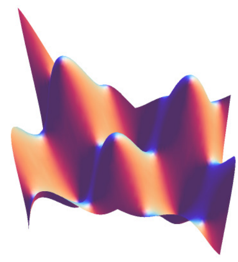
Refer to caption — Figure 4: $L^{2}$ approximation of the smooth function (44) (middle column) on two different bilinearly parameterized multi-patch domains $\Omega$ (left column) using spline spaces $\mathcal{W}^{s}$ for a global smoothness $s=1,\ldots,4$ , and a mesh size $h=\frac{1}{2^{L}}$ , with $L=0,1,\ldots,5$ or $L=0,1,\ldots,6$ , for a spline degree $p=2s+1$ and for an inner patch regularity $r=s$ . The resulting relative $L^{2}$ errors (right column) are visualized with respect to the number of degrees of freedom (NDOF).

The goal of this section is to numerically study the approximation power of the isogeometric spline space $\mathcal{W}^{s}$ by performing $L^{2}$ approximation over the two bilinearly parameterized multi-patch domains $\Omega$ given in Fig. 4 (left column). More precisely, we will approximate the smooth function

z(\boldsymbol{x})=z(x_{1},x_{2})=4\cos(2x_{1})\sin(2x_{2}),

(44)

visualized in Fig. 4 (middle column) on these two multi-patch domains, by employing isogeometric spline spaces $\mathcal{W}^{s}$ for a global smoothness $s=1,\ldots,4$ , and a mesh size $h=\frac{1}{2^{L}}$ , with $L=0,1,\ldots,5$ or $L=0,1,\ldots,6$ , for a spline degree $p=2s+1$ and for an inner patch regularity $r=s$ . Let $\{\phi_{j}\}_{j=0}^{\dim\mathcal{W}^{s}-1}$ be a basis of such an isogeometric spline space $\mathcal{W}^{s}$ , then we compute an approximation

z_{h}(\boldsymbol{x})=\sum_{j=0}^{\dim\mathcal{W}^{s}-1}c_{j}\phi_{j}(\boldsymbol{x}),\quad c_{j}\in\mathbb{R},

of the function $z$ , by minimizing the objective function

\int_{\Omega}(z_{h}(\boldsymbol{x})-z(\boldsymbol{x}))^{2}\mathrm{d}\boldsymbol{x}.

Finding a solution of this minimization problem is equivalent to solving the linear system

M\boldsymbol{c}=\boldsymbol{z},\quad\boldsymbol{c}=(c_{j})_{j=0}^{\dim\mathcal{W}^{s}-1},

where $M$ is the mass matrix with the single entries

m_{j_{1},j_{2}}=\int_{\Omega}\phi_{j_{1}}(\boldsymbol{x})\phi_{j_{2}}(\boldsymbol{x})\mathrm{d}\boldsymbol{x},

(45)

and $\boldsymbol{z}$ is the right side vector with the single entries

z_{j}=\int_{\Omega}z(\boldsymbol{x})\phi_{j}(\boldsymbol{x})\mathrm{d}\boldsymbol{x}.

(46)

Using the relation $f_{j}^{(i)}=\phi_{j}\circ\boldsymbol{F}^{(i)}$ , $i\in\mathcal{I}_{\Omega}$ , the entries (45) and (46) can be computed via

m_{j_{1},j_{2}}=\sum_{i\in\mathcal{I}_{\Omega}}\int_{[0,1]^{2}}f_{j_{1}}^{(i)}(\xi_{1},\xi_{2})f_{j_{2}}^{(i)}(\xi_{1},\xi_{2})|\det({\rm J}\boldsymbol{F}^{(i)}(\xi_{1},\xi_{2}))|\mathrm{d}\xi_{1}\mathrm{d}\xi_{2},

and

z_{j}=\sum_{i\in\mathcal{I}_{\Omega}}\int_{[0,1]^{2}}z(\boldsymbol{F}^{(i)}(\xi_{1},\xi_{2}))f_{j}^{(i)}(\xi_{1},\xi_{2})|\det({\rm J}\boldsymbol{F}^{(i)}(\xi_{1},\xi_{2}))|\mathrm{d}\xi_{1}\mathrm{d}\xi_{2},

respectively.

While in case of the bilinearly parameterized two-patch domain, see Fig. 4 (top row and left column), the basis for the space $\mathcal{W}^{s}$ is generated as described in Section 3.2, in case of the bilinearly parameterized three-patch domain, see Fig. 4 (bottom row and left column), the basis is constructed as explained in Section 4. In the latter case, the design of the vertex subspaces $\mathcal{W}^{s}_{\Xi^{(i)}}$ has to be slightly modified in case of a mesh size $\frac{p-r-s}{3s-r+1}\leq h\leq 1$ for boundary vertices. Namely, the vertex subspace $\mathcal{W}^{s}_{\Xi^{(i)}}$ for a boundary vertex $\Xi^{(i)}$ is then just generated by those corresponding functions $\phi_{\Gamma^{(i)};j_{1},j_{2}}$ and/or $\phi_{\Omega^{(i)};j_{1},j_{2}}$ , which have not been already used to construct the vertex subspace for another vertex especially for the inner vertex.

Fig. 4 (right column) displays the resulting relative $L^{2}$ errors with respect to the number of degrees of freedom (NDOF) by performing $L^{2}$ approximation on the two different bilinearly parameterized multi-patch domains. In all cases, the numerical results indicate a convergence rate of optimal order of $\mathcal{O}(h^{p+1})$ in the $L^{2}$ norm. In case of the three-patch domain, the shown results have been obtained by employing the minimal determing set approach for the construction of the vertex subspaces. However, the use of the alternative interpolation strategy instead would lead to a nearly indistinguishable result but which is not presented here. The number of degrees of freedom, i.e. the dimensions of the obtained isogeometric spline spaces $\mathcal{W}^{s}$ for the two different multi-patch domains are reported in Table 1.

	Two-patch domain
$h$	$p=3$ , $s=r=1$	$p=5$ , $s=r=2$	$p=7$ , $s=r=3$	$p=9$ , $s=r=4$
$1$	23	51	90	140
$\frac{1}{2}$	57	126	222	345
$\frac{1}{4}$	173	384	678	1055
$\frac{1}{8}$	597	1332	2358	3675
$\frac{1}{16}$	2213	4956	8790	13715
$\frac{1}{32}$	8517	19116	33942	52995
	Three-patch domain
$h$	$p=3$ , $s=r=1$	$p=5$ , $s=r=2$	$p=7$ , $s=r=3$	$p=9$ , $s=r=4$
$1$	24 (24)	52 (51)	90 (88)	139 (135)
$\frac{1}{2}$	66 (66)	142 (141)	246 (244)	379 (375)
$\frac{1}{4}$	222 (222)	484 (483)	846 (844)	1309 (1305)
$\frac{1}{8}$	822 (822)	1816 (1815)	3198 (3196)	4969 (4965)
$\frac{1}{16}$	3174 (3174)	7072 (7071)	12510 (12508)	19489 (19485)
$\frac{1}{32}$	12486 (12486)	27952 (27951)	49566 (49564)	77329 (77325)

Table 1: The number of degrees of freedom, i.e. the dimensions of the generated isogeometric spline spaces

\mathcal{W}^{s}

in Section 6 for a mesh size

h=\frac{1}{2^{L}}

L=0,1,\ldots,5

, for the two bilinearly parameterized multi-patch domains shown in Fig. 4 (left column). In case of the three-patch domain, the number in the brackets represents the dimension when using the alternative interpolation strategy for the construction of the vertex subspaces instead of the minimal determining set approach.

7 Conclusion

We have studied the space of $C^{s}$ -smooth ( $s\geq 1$ ) isogeometric spline functions on planar, bilinearly parameterized multi-patch domains and have presented the construction of a particular subspace of this $C^{s}$ -smooth isogeometric spline space. The use of the $C^{s}$ -smooth subspace is advantageous compared to the use of the entire $C^{s}$ -smooth space, since the design of the subspace is simple and works uniformly for all possible multi-patch configurations, and furthermore, the numerical experiments by performing $L^{2}$ approximation indicate that the subspace already possesses optimal approximation properties.

The construction of the $C^{s}$ -smooth subspace and of an associated simple and locally supported basis is firstly described for the case of two-patch domains, and is then extended to the case of multi-patch domains with more than two patches and with possibly extraordinary vertices. In the latter case, the $C^{s}$ -smooth subspace is generated as the direct sum of spaces corresponding to the individual patches, edges and vertices.

Moreover, a possible generalization of our approach to a more general class of planar multi-patch parameterizations, called bilinear-like $G^{s}$ multi-patch geometries, is briefly explained. This class of multi-patch parameterizations provides the possibility to model multi-patch domains with curved interfaces and boundaries. A detailed study of this class of geometries is beyond the scope of the paper and is a topic of our future research. Further open problems which are worth to study are e.g. the theoretical investigation of the approximation properties of the constructed $C^{s}$ -smooth isogeometric spline space, the use of the $C^{s}$ -smooth isogeometric spline functions for applications which require functions of high continuity such as solving fourth order PDEs via isogeometric collocation, and the extension of our approch to multi-patch shells and volumes.

Acknowledgements.

M. Kapl has been partially supported by the Austrian Science Fund (FWF) through the project P 33023. V. Vitrih has been partially supported by the research program P1-0404 and research projects J1-9186, J1-1715 from ARRS, Republic of Slovenia. This support is gratefully acknowledged.

Conflict of interest

The authors declare that they have no conflict of interest.

References

(1) Anitescu, C., Jia, Y., Zhang, Y.J., Rabczuk, T.: An isogeometric collocation method using superconvergent points. Comput. Methods Appl. Mech. Engrg. 284, 1073–1097 (2015)
(2) Auricchio, F., Beirão da Veiga, L., Buffa, A., Lovadina, C., Reali, A., Sangalli, G.: A fully ”locking-free” isogeometric approach for plane linear elasticity problems: a stream function formulation. Comput. Methods Appl. Mech. Engrg. 197(1), 160–172 (2007)
(3) Auricchio, F., Beirão da Veiga, L., Hughes, T.J.R., Reali, A., Sangalli, G.: Isogeometric collocation methods. Math. Models Methods Appl. Sci. 20(11), 2075–2107 (2010)
(4) Bartezzaghi, A., Dedè, L., Quarteroni, A.: Isogeometric analysis of high order partial differential equations on surfaces. Comput. Methods Appl. Mech. Engrg. 295, 446 – 469 (2015)
(5) Beirão da Veiga, L., Buffa, A., Sangalli, G., Vázquez, R.: Mathematical analysis of variational isogeometric methods. Acta Numerica 23, 157–287 (2014)
(6) Benson, D.J., Bazilevs, Y., Hsu, M.C., Hughes, T.J.: A large deformation, rotation-free, isogeometric shell. Comput. Methods Appl. Mech. Engrg. 200(13), 1367–1378 (2011)
(7) Bercovier, M., Matskewich, T.: Smooth Bézier Surfaces over Unstructured Quadrilateral Meshes. Lecture Notes of the Unione Matematica Italiana, Springer (2017)
(8) Blidia, A., Mourrain, B., Villamizar, N.: G¹-smooth splines on quad meshes with 4-split macro-patch elements. Comput. Aided Geom. Des. 52–-53, 106 – 125 (2017)
(9) Blidia, A., Mourrain, B., Xu, G.: Geometrically smooth spline bases for data fitting and simulation. Comput. Aided Geom. Des. 78, 101814 (2020)
(10) Chan, C., Anitescu, C., Rabczuk, T.: Isogeometric analysis with strong multipatch C¹-coupling. Comput. Aided Geom. Design 62, 294–310 (2018)
(11) Chan, C., Anitescu, C., Rabczuk, T.: Strong multipatch C¹-coupling for isogeometric analysis on 2D and 3D domains. Comput. Methods Appl. Mech. Engrg. 357, 112599 (2019)
(12) Collin, A., Sangalli, G., Takacs, T.: Analysis-suitable G¹ multi-patch parametrizations for C¹ isogeometric spaces. Comput. Aided Geom. Des. 47, 93 – 113 (2016)
(13) Cottrell, J.A., Hughes, T.J.R., Bazilevs, Y.: Isogeometric Analysis: Toward Integration of CAD and FEA. John Wiley & Sons, Chichester, England (2009)
(14) Farin, G.: Curves and Surfaces for Computer-Aided Geometric Design. Academic Press (1997)
(15) Fischer, P., Klassen, M., Mergheim, J., Steinmann, P., Müller, R.: Isogeometric analysis of 2D gradient elasticity. Comput. Mech. 47(3), 325–334 (2011)
(16) Gómez, H., Calo, V.M., Bazilevs, Y., Hughes, T.J.: Isogeometric analysis of the Cahn–Hilliard phase-field model. Comput. Methods Appl. Mech. Engrg. 197(49), 4333–4352 (2008)
(17) Gomez, H., Calo, V.M., Hughes, T.J.R.: Isogeometric analysis of Phase–Field models: Application to the Cahn–Hilliard equation. In: ECCOMAS Multidisciplinary Jubilee Symposium: New Computational Challenges in Materials, Structures, and Fluids, pp. 1–16. Springer Netherlands (2009)
(18) Gomez, H., De Lorenzis, L.: The variational collocation method. Comput. Methods Appl. Mech. Engrg. 309, 152–181 (2016)
(19) Gomez, H., Nogueira, X.: An unconditionally energy-stable method for the phase field crystal equation. Comput. Methods Appl. Mech. Engrg. 249 – 252, 52 – 61 (2012)
(20) Groisser, D., Peters, J.: Matched G^k-constructions always yield C^k-continuous isogeometric elements. Comput. Aided Geom. Des. 34, 67 – 72 (2015)
(21) Hernández Encinas, L., Muñoz Masqué, J.: A short proof of the generalized Faà di Bruno’s formula. Appl. Math. Lett. 16(6), 975–979 (2003)
(22) Hoschek, J., Lasser, D.: Fundamentals of computer aided geometric design. A K Peters Ltd., Wellesley, MA (1993)
(23) Hughes, T.J.R., Cottrell, J.A., Bazilevs, Y.: Isogeometric analysis: CAD, finite elements, NURBS, exact geometry and mesh refinement. Comput. Methods Appl. Mech. Engrg. 194(39-41), 4135–4195 (2005)
(24) Kapl, M., Buchegger, F., Bercovier, M., Jüttler, B.: Isogeometric analysis with geometrically continuous functions on planar multi-patch geometries. Comput. Methods Appl. Mech. Engrg. 316, 209 – 234 (2017)
(25) Kapl, M., Sangalli, G., Takacs, T.: Dimension and basis construction for analysis-suitable G¹ two-patch parameterizations. Comput. Aided Geom. Des. 52–53, 75 – 89 (2017)
(26) Kapl, M., Sangalli, G., Takacs, T.: Construction of analysis-suitable G¹ planar multi-patch parameterizations. Comput.-Aided Des. 97, 41–55 (2018)
(27) Kapl, M., Sangalli, G., Takacs, T.: Isogeometric analysis with C¹ functions on unstructured quadrilateral meshes. The SMAI journal of computational mathematics 5, 67–86 (2019)
(28) Kapl, M., Sangalli, G., Takacs, T.: An isogeometric C¹ subspace on unstructured multi-patch planar domains. Comput. Aided Geom. Des. 69, 55–75 (2019)
(29) Kapl, M., Vitrih, V.: Space of C²-smooth geometrically continuous isogeometric functions on planar multi-patch geometries: Dimension and numerical experiments. Comput. Math. Appl. 73(10), 2319––2338 (2017)
(30) Kapl, M., Vitrih, V.: Space of C²-smooth geometrically continuous isogeometric functions on two-patch geometries. Comput. Math. Appl. 73(1), 37 – 59 (2017)
(31) Kapl, M., Vitrih, V.: Dimension and basis construction for ${C}^{2}$ -smooth isogeometric spline spaces over bilinear-like ${G}^{2}$ two-patch parameterizations. J. Comput. Appl. Math. 335, 289–311 (2018)
(32) Kapl, M., Vitrih, V.: Solving the triharmonic equation over multi-patch planar domains using isogeometric analysis. J. Comput. Appl. Math. 358, 385–404 (2019)
(33) Kapl, M., Vitrih, V.: Isogeometric collocation on planar multi-patch domains. Comput. Methods Appl. Mech. Engrg. 360, 112684 (2020)
(34) Kapl, M., Vitrih, V., Jüttler, B., Birner, K.: Isogeometric analysis with geometrically continuous functions on two-patch geometries. Comput. Math. Appl. 70(7), 1518 – 1538 (2015)
(35) Karčiauskas, K., Nguyen, T., Peters, J.: Generalizing bicubic splines for modeling and IGA with irregular layout. Comput.-Aided Des. 70, 23 – 35 (2016)
(36) Karčiauskas, K., Peters, J.: Refinable ${G}^{1}$ functions on ${G}^{1}$ free-form surfaces. Comput. Aided Geom. Des. 54, 61–73 (2017)
(37) Karčiauskas, K., Peters, J.: Refinable bi-quartics for design and analysis. Comput.-Aided Des. pp. 204–214 (2018)
(38) Khakalo, S., Niiranen, J.: Isogeometric analysis of higher-order gradient elasticity by user elements of a commercial finite element software. Comput.-Aided Des. 82, 154 – 169 (2017)
(39) Kiendl, J., Bazilevs, Y., Hsu, M.C., Wüchner, R., Bletzinger, K.U.: The bending strip method for isogeometric analysis of Kirchhoff-Love shell structures comprised of multiple patches. Comput. Methods Appl. Mech. Engrg. 199(35), 2403–2416 (2010)
(40) Kiendl, J., Bletzinger, K.U., Linhard, J., Wüchner, R.: Isogeometric shell analysis with Kirchhoff-Love elements. Comput. Methods Appl. Mech. Engrg. 198(49), 3902–3914 (2009)
(41) Kiendl, J., Hsu, M.C., Wu, M.C.H., Reali, A.: Isogeometric Kirchhoff–Love shell formulations for general hyperelastic materials. Comput. Methods Appl. Mech. Engrg. 291, 280 – 303 (2015)
(42) Lai, M.J., Schumaker, L.L.: Spline functions on triangulations, Encyclopedia of Mathematics and its Applications, vol. 110. Cambridge University Press, Cambridge (2007)
(43) Liu, J., Dedè, L., John A Evans, J.A., Borden, M.J., Hughes, T.J.R.: Isogeometric analysis of the advective Cahn–Hilliard equation: Spinodal decomposition under shear flow. Journal of Computational Physics 242, 321 – 350 (2013)
(44) Makvandi, R., Reiher, J.C., Bertram, A., Juhre, D.: Isogeometric analysis of first and second strain gradient elasticity. Comput. Mech. 61(3), 351–363 (2018)
(45) Montardini, M., Sangalli, G., Tamellini, L.: Optimal-order isogeometric collocation at Galerkin superconvergent points. Comput. Methods Appl. Mech. Engrg. 316, 741–757 (2017)
(46) Mourrain, B., Vidunas, R., Villamizar, N.: Dimension and bases for geometrically continuous splines on surfaces of arbitrary topology. Comput. Aided Geom. Des. 45, 108 – 133 (2016)
(47) Nguyen, T., Karčiauskas, K., Peters, J.: ${C}^{1}$ finite elements on non-tensor-product 2d and 3d manifolds. Applied Mathematics and Computation 272, 148 – 158 (2016)
(48) Nguyen, T., Peters, J.: Refinable ${C}^{1}$ spline elements for irregular quad layout. Comput. Aided Geom. Des. 43, 123 – 130 (2016)
(49) Niiranen, J., Khakalo, S., Balobanov, V., Niemi, A.H.: Variational formulation and isogeometric analysis for fourth-order boundary value problems of gradient-elastic bar and plane strain/stress problems. Comput. Methods Appl. Mech. Engrg. 308, 182–211 (2016)
(50) Niiranen, J., Kiendl, J., Niemi, A.H., Reali, A.: Isogeometric analysis for sixth-order boundary value problems of gradient-elastic Kirchhoff plates. Comput. Methods Appl. Mech. Engrg. 316, 328––348 (2017)
(51) Peters, J.: Geometric continuity. In: Handbook of computer aided geometric design, pp. 193–227. North-Holland, Amsterdam (2002)
(52) Tagliabue, A., Dedè, L., Quarteroni, A.: Isogeometric analysis and error estimates for high order partial differential equations in fluid dynamics. Computers & Fluids 102, 277 – 303 (2014)
(53) Toshniwal, D., Speleers, H., Hiemstra, R., Hughes, T.J.R.: Multi-degree smooth polar splines: A framework for geometric modeling and isogeometric analysis. Comput. Methods Appl. Mech. Engrg. (2016)
(54) Toshniwal, D., Speleers, H., Hughes, T.J.R.: Smooth cubic spline spaces on unstructured quadrilateral meshes with particular emphasis on extraordinary points: Geometric design and isogeometric analysis considerations. Comput. Methods Appl. Mech. Engrg. 327, 411–458 (2017)
(55) Verhoosel, C.V., Scott, M.A., Hughes, T.J.R., de Borst, R.: An isogeometric analysis approach to gradient damage models. Internat. J. Numer. Methods Engrg. 86(1), 115–134 (2011)



Multi-patch domain $\Omega$	Smooth function $z$	Relative $L^{2}$ errors

CsC^{s}-smooth isogeometric spline spaces over planar multi-patch parameterizations

Abstract

Keywords:

MSC

1 Introduction

2 The multi-patch setting and CsC^{s}-smooth isogeometric spline spaces

3 CsC^{s}-smooth isogeometric spline spaces over two-patch domains

3.1 GsG^{s}-smoothness of graph surfaces

Remark 1

Theorem 3.1

Example 1

Example 2

Proposition 1

3.2 Construction of CsC^{s}-smooth isogeometric spline spaces

Theorem 3.2

Proof

Theorem 3.3

Proof

4 CsC^{s}-smooth isogeometric spaces over multi-patch domains

4.1 The patch and edge subspaces

4.2 The vertex subspaces

Remark 2

5 Beyond bilinear parameterization

Definition 1

6 Examples

7 Conclusion

Acknowledgements.

Conflict of interest

References

$C^{s}$ -smooth isogeometric spline spaces over planar multi-patch parameterizations

2 The multi-patch setting and $C^{s}$ -smooth isogeometric spline spaces

3 $C^{s}$ -smooth isogeometric spline spaces over two-patch domains

3.1 $G^{s}$ -smoothness of graph surfaces

3.2 Construction of $C^{s}$ -smooth isogeometric spline spaces

4 $C^{s}$ -smooth isogeometric spaces over multi-patch domains