Complexity Aspects of Local Minima
and Related NotionsThanks: This work was supported partially by an AFOSR MURI award, the DARPA Young Faculty Award, the Princeton SEAS Innovation Award, the NSF CAREER Award, the Google Faculty Award, and the Sloan Fellowship.

Complexity Aspects of Local Minima and Related NotionsThanks: This work was supported partially by an AFOSR MURI award, the DARPA Young Faculty Award, the Princeton SEAS Innovation Award, the NSF CAREER Award, the Google Faculty Award, and the Sloan Fellowship.

Complexity Aspects of Local Minima
and Related NotionsThanks: This work was supported partially by an AFOSR MURI award, the DARPA Young Faculty Award, the Princeton SEAS Innovation Award, the NSF CAREER Award, the Google Faculty Award, and the Sloan Fellowship.

1 Introduction

2 NP-hardness Results

3 Checking Local Minimality of a Point for a Cubic Polynomial

4 On the Geometry of Local Minima of Cubic Polynomials

5 Complexity Justifications for an Exact SDP Oracle

6 Finding Local Minima of Cubic Polynomials

7 Conclusions and Future Directions

References

1 Introduction

2 NP-hardness Results

3 Checking Local Minimality of a Point for a Cubic Polynomial

4 On the Geometry of Local Minima of Cubic Polynomials

5 Complexity Justifications for an Exact SDP Oracle

6 Finding Local Minima of Cubic Polynomials

1.1 Organization and Main Contributions of the Paper

1.2 Preliminaries and Notation

3.1 Preliminaries on Cubic Polynomials

3.2 Local Minimality of a Point for a Cubic Polynomial

3.3 Examples

4.1 Convexity of the Set of Local Minima

4.2 Local Minima and Solutions to a “Convex” Problem

4.3 Distinction Between Local Minima and Second-Order Points

4.4 Spectrahedra and Convexity Regions of Cubic Polynomials

6.1 Preliminaries from Semidefinite and Sum of Squares Optimization

6.2 A Sum of Squares Approach for Finding Second-Order Points

6.3 A Simplified Semidefinite Representation of Second-Order Points and an Algorithm for Finding Local Minima

7.1 Approximate Local Minima

7.2 Unregularized Third-Order Newton Methods

1.1 Organization and Main Contributions of the Paper

1.2 Preliminaries and Notation

3.1 Preliminaries on Cubic Polynomials

3.2 Local Minimality of a Point for a Cubic Polynomial

3.3 Examples

4.1 Convexity of the Set of Local Minima

4.2 Local Minima and Solutions to a “Convex” Problem

4.3 Distinction Between Local Minima and Second-Order Points

4.4 Spectrahedra and Convexity Regions of Cubic Polynomials

6.1 Preliminaries from Semidefinite and Sum of Squares Optimization

6.2 A Sum of Squares Approach for Finding Second-Order Points

6.1.1 The Oracle E-SDP

6.1.2 Overview of Sum of Squares Polynomials

6.3.1 A Simplified Sos Relaxation

6.3.2 Combining the SDP in (27) with its Dual

6.3.3 An Algorithm for Finding Local Minima

6.1.1 The Oracle E-SDP

6.1.2 Overview of Sum of Squares Polynomials

Keywords:

Keywords:

Abstract

Theorem 2.1.

Proof.

Theorem 2.2.

Proof.

Theorem 2.3 ([2]).

Theorem 3.1.

Remark 3.1.

Lemma 3.2.

Proof.

Proof (of Theorem 3.1).

Remark 3.2.

Theorem 3.3.

Proof.

Corollary 3.4.

Proof.

Corollary 3.5.

Proof.

Example 3.1.

Example 3.2.

Example 3.3.

Lemma 4.1.

Proof.

Lemma 4.2.

Proof.

Theorem 4.3.

Proof.

Lemma 4.4.

Proof.

Theorem 4.5.

Proof.

Remark 4.1.

Definition 4.6.

Theorem 4.7.

Proof.

Remark 4.2.

Corollary 4.8.

Proof.

Definition 4.9.

Theorem 4.10.

Proof.

Corollary 4.11.

Proof.

Theorem 4.12.

Proof.

Definition 5.1.

Definition 5.2.

Theorem 5.3.

Proof.

Theorem 5.4.

Proof.

Example 5.1.

Example 5.2.

Example 5.3.

Lemma 6.1.

Proof.

Theorem 6.2.

Proof.

Theorem 6.3.

Proof.

Theorem 6.4.

Proof.

Corollary 6.5.

Proof.

Remark 6.1.

Theorem 7.1.

Proof.

Abstract

Theorem 2.1.

Proof.

Theorem 2.2.

Proof.

Theorem 2.3 ([2]).

Theorem 3.1.

Remark 3.1.

Lemma 3.2.

Proof.

Proof (of Theorem 3.1).

Remark 3.2.

Theorem 3.3.

Proof.

Corollary 3.4.

Proof.

Corollary 3.5.

Proof.

Example 3.1.

Example 3.2.

Example 3.3.

Lemma 4.1.

Proof.

Lemma 4.2.

Proof.

Theorem 4.3.

Proof.

Lemma 4.4.

Proof.

Theorem 4.5.

Proof.

Remark 4.1.

Definition 4.6.

Theorem 4.7.

Proof.

Remark 4.2.

Corollary 4.8.

Proof.

Definition 4.9.

Theorem 4.10.

Proof.

Corollary 4.11.

Proof.

Theorem 4.12.

Proof.

Definition 5.1.

Definition 5.2.

Theorem 5.3.

Proof.

Theorem 5.4.

Proof.

Example 5.1.

Example 5.2.

Example 5.3.

Lemma 6.1.

Proof.

Theorem 6.2.

Proof.

Theorem 6.3.

Amir Ali Ahmadi Thanks: Department of Operations Research and Financial Engineering, Princeton University; aaa@princeton.edu Jeffrey Zhang Thanks: Department of Mathematical Sciences, Carnegie Mellon University; jeffz@cmu.edu

We consider the notions of (i) critical points, (ii) second-order points, (iii) local minima, and (iv) strict local minima for multivariate polynomials. For each type of point, and as a function of the degree of the polynomial, we study the complexity of deciding (1) if a given point is of that type, and (2) if a polynomial has a point of that type. Our results characterize the complexity of these two questions for all degrees left open by prior literature. Our main contributions reveal that many of these questions turn out to be tractable for cubic polynomials. In particular, we present an efficiently-checkable necessary and sufficient condition for local minimality of a point for a cubic polynomial. We also show that a local minimum of a cubic polynomial can be efficiently found by solving semidefinite programs of size linear in the number of variables. By contrast, we show that it is strongly NP-hard to decide if a cubic polynomial has a critical point. We also prove that the set of second-order points of any cubic polynomial is a spectrahedron, and conversely that any spectrahedron is the projection of the set of second-order points of a cubic polynomial. In our final section, we briefly present a potential application of finding local minima of cubic polynomials to the design of a third-order Newton method.

Local minima, critical and second-order points, computational complexity, polynomial optimization, sum of squares polynomials, semidefinite programming.

We are concerned in this paper with algorithmic questions around the following four types of points associated with a sufficiently smooth function $f:\mathbb{R}^{n}\to\mathbb{R}$ :

(i)

a critical point, i.e., a point $x$ where the gradient $\nabla f(x)$ is zero,
(ii)

a second-order point, i.e., a point $x$ where $\nabla f(x)=0$ and the Hessian $\nabla^{2}f(x)$ is positive semidefinite (psd), i.e. has nonnegative eigenvalues,
(iii)

a local minimum, i.e., a point $x$ for which there exists a scalar $\epsilon>0$ such that $f(x)\leq f(y)$ for all $y$ with $\|y-x\|\leq\epsilon$ ,
(iv)

a strict local minimum, i.e., a point $x$ for which there exists a scalar $\epsilon>0$ such that $f(x)<f(y)$ for all $y\neq x$ with $\|y-x\|\leq\epsilon$ .

We note the following straightforward implications between (i)-(iv):

strict local minimum $\Rightarrow$ local minimum $\Rightarrow$ second-order point $\Rightarrow$ critical point.

Notions (i)-(iv) appear ubiquitously in nonconvex continuous optimization as surrogates for global minima. This is because it is well understood that finding a global minimum of $f$ is in general an intractable problem.

In this paper, with regard to each of the four notions above, we study the complexity of answering the following questions:

Q1:

Given a function $f:\mathbb{R}^{n}\to\mathbb{R}$ and a point $x\in\mathbb{R}^{n}$ , is $x$ of a given type (i)-(iv)?
Q2:

Given a function $f:\mathbb{R}^{n}\to\mathbb{R}$ , does $f$ have a point of a given type (i)-(iv) (and if so, can one be found efficiently)?

Note that a priori there are no complexity implications between these two questions. For example, an algorithm for verifying that a given point is a local minimum does not necessarily provide instructions on how one would find a local minimum. Conversely, even if local minimality of a given point cannot always be efficiently certified, that does not rule out the existence of algorithms that can efficiently find particular local minima that are easy to certify; see e.g. Question 3 of [21]. Thus, in general, these two questions need to be studied separately.

The functions $f$ for which we study Q1 and Q2 are (multivariate) polynomials. Polynomial functions appear throughout optimization theory either as exact models of objective functions or as approximations thereof. For example, many optimization algorithms involve minimizing Taylor expansions of more complicated functions as a subroutine. As is well known, polynomials can approximate continuous functions arbitrarily well over compact sets. This makes them a particularly suitable candidate for studying local notions such as (i)-(iv). In addition to these representation reasons, since polynomial functions of a given degree are finitely parameterized, they allow for a convenient setting for a formal study of complexity questions. For example, one can study the complexity of Q1 and Q2 in the Turing model of computation, where the size of a given instance is determined by the number of bits required to write down the coefficients of the polynomial (and, in the case of Q1, the entries of the point $x$ ), which are taken to be rational numbers. For the purposes of analyzing the complexity of these two questions for polynomial functions, we consider the relevant setting in applications where the degree¹¹ 1 In this paper, by a degree- $d$ polynomial, we mean a polynomial whose monomials have degree at most $d$ . All our complexity results hold for this convention, as well as for the convention which requires a degree- $d$ polynomial to have at least one monomial of degree $d$ with a nonzero coefficient. of the polynomial is fixed and its number of variables increases. We are interested in the existence or non-existence of efficient algorithms for solving these questions in this setting, as established theory (e.g. quantifier elimination theory [28, 27]) already yields exponential-time algorithms for them.

Let us first comment on the complexity of Q1 and Q2 for some simple and classical cases. For Q1, checking whether a given point is a critical point of a polynomial function (of any degree) can trivially be done in polynomial time simply by evaluating the gradient at that point. To check that a given point is a second-order point, one can additionally compute the Hessian matrix at that point and check that it is positive semidefinite. This can be done in polynomial time, e.g., by performing Gaussian pivot steps along the main diagonal of the matrix [15, Section 1.3.1] or by computing its characteristic polynomial and checking that the signs of its coefficients alternate [13, p. 403]. Since for affine or quadratic polynomials, any second-order point is a local minimum, the only remaining case for Q1 is that of strict local minima. Affine polynomials never have strict local minima, making the question uninteresting. A point is a strict local minimum of a quadratic polynomial if and only if it is a critical point and the associated Hessian matrix is positive definite (pd), i.e., has positive eigenvalues. The latter property can be checked in polynomial time, for example by computing the leading principal minors of the Hessian and checking that they are all positive. As for Q2, the affine case is again uninteresting since there is a critical point (which will also be a second-order point and a local minimum) if and only if the coefficients of all degree-one monomials are zero. For quadratic polynomials, since the entries of the gradient are affine, searching for critical points can be done in polynomial time by solving a linear system. A candidate critcal point will be a second-order point (and a local minimum) if and only if the Hessian is psd, and a strict local minimum if and only if the Hessian is pd.

Other than the aforementioned cases, the only prior result in the literature that we are aware of is due to Murty and Kabadi [14], which settles the complexity of Q1 for degree-4 polynomials. Our contribution in this paper is to settle the complexity of the remaining cases for both Q1 and Q2. A summary of the results is presented in Table 1 and Table 2. Entries denoted by “P” indicate that the problem can be solved in polynomial time. The notation “SDP” indicates that the problem of interest can be reduced to solving either one or polynomially-many semidefinite programs (SDP) whose sizes are polynomial in the size of the input. (In fact, the reduction also goes in the other direction for second-order points and local minima; see Theorems 5.3 and 5.4.) Finally, we recall that a strong NP-hardness result implies that the problem of interest remains NP-hard even if the size (i.e. bit length) of the coefficients of the polynomial is $O(\log(n))$ , where $n$ is the number of variables. Therefore, unless P=NP, even a pseudo-polynomial time algorithm (i.e., an algorithm whose running time is polynomial in the magnitude of the coefficients, but not necessarily their bit length) cannot exist for the indicated problems in these tables. See [9] or [1, Section 2] for more details on the distinction between weakly and strongly NP-hard problems.

Q1: property vs. degree	$1$	$2$	$3$	$\geq 4$
Critical point	P	P	P	P
Second-order point	P	P	P	P
Local minimum	P	P	P	strongly NP-hard [14]²² 2 The proof in [14] is based on a reduction from the “matrix copositivity” problem. However, [14] only shows that this problem (and thus deciding if a quartic polynomial has a local minimum) is weakly NP-hard, since the reduction to matrix copositivity there is from the weakly NP-hard problem of Subset Sum. Nonetheless, their result can be strengthened by observing that testing matrix copositivity is in fact strongly NP-hard. This claim is implicit, e.g., in [8, Corollary 2.4]. The NP-hardness of testing whether a point is a strict local minimum of a quartic polynomial is not explicitly stated in [14], though it follows in the weak sense from the weak NP-hardness of Problem 8 of [14]. Again, with some work, this can be strengthened to a strong NP-hardness result.
			(Theorem 3.3)
Strict local minimum	P	P	P	strongly NP-hard [14]²² 2 The proof in [14] is based on a reduction from the “matrix copositivity” problem. However, [14] only shows that this problem (and thus deciding if a quartic polynomial has a local minimum) is weakly NP-hard, since the reduction to matrix copositivity there is from the weakly NP-hard problem of Subset Sum. Nonetheless, their result can be strengthened by observing that testing matrix copositivity is in fact strongly NP-hard. This claim is implicit, e.g., in [8, Corollary 2.4]. The NP-hardness of testing whether a point is a strict local minimum of a quartic polynomial is not explicitly stated in [14], though it follows in the weak sense from the weak NP-hardness of Problem 8 of [14]. Again, with some work, this can be strengthened to a strong NP-hardness result.
			(Corollary 3.5)

Table 1: Complexity of deciding whether a given point is of a certain type, based on the degree of the polynomial. Entries without a reference are classical.

Q2: property vs. degree	$1$	$2$	$3$	$\geq 4$
Critical point	P	P	strongly NP-hard	strongly NP-hard
			(Theorem 2.1)	(Theorem 2.1)
Second-order point	P	P	SDP	strongly NP-hard
			(Corollary 6.5)	(Theorem 2.2)
Local minimum	P	P	SDP	strongly NP-hard
			(Algorithm 2)	(Theorem 2.3)³³ 3 The proof of Theorem 2.3 will appear in an upcoming paper by the authors, as a corollary of it answers a question originally posed in [21]; see Section 2.
Strict local minimum	P	P	SDP	strongly NP-hard
			(Algorithm 2, Remark 6.1)	(Theorem 2.3)³³ 3 The proof of Theorem 2.3 will appear in an upcoming paper by the authors, as a corollary of it answers a question originally posed in [21]; see Section 2.

Table 2: Complexity of deciding whether a polynomial has a point of a certain type, based on the degree of the polynomial. Entries without a reference are classical.

The majority of the technical work in this paper is spent on the case of cubic polynomials. It is somewhat surprising that many of the problems of interest to us are tractable for cubics, especially the search for local minima. This is in contrast to the intractability of other interesting problems related to cubic polynomials, e.g., minimizing them over the unit sphere [16], or checking their convexity over a box [1]. It is also interesting to note that second-order points of cubic polynomials are easier to find than their critical points, despite being a more restrictive type of point. This shows that the right approach to finding second-order points involves bypassing the search for critical points as an initial step.

Section 2 covers the NP-hardness results from Table 2. The remainder of the paper is devoted to our results on cubic polynomials, which fills in the remaining entries of Tables 1 and 2. In Section 3, we give a characterization of local minima of cubic polynomials (Theorem 3.1) and show that it can be checked in polynomial time (Theorem 3.3). In Section 4, we give some geometric facts about local minima of cubic polynomials. For example, we show that the set of local minima of a cubic polynomial $p$ is convex (Theorem 4.3), and we relate this set to the second-order points of $p$ and to the set of minima of $p$ over points where $\nabla^{2}p$ is positive semidefinite (Theorem 4.7 and Theorem 4.10). In Section 4.4, we show that the interior of any spectrahedron is the projection of the local minima of some cubic polynomial (Theorem 4.12). In Section 5, we use this result to show that deciding if a cubic polynomial has a local minimum or a second-order point is at least as hard as some semidefinite feasibility problems.

In Section 6, we start from a “sum of squares” approach to finding second-order points of a cubic polynomial (Theorem 6.2 and Theorem 6.3), and build upon it (Section 6.3) to arrive at an efficient semidefinite representation of these points (Corollary 6.5). This also leads to an algorithm for finding local minima of cubic polynomials by solving polynomially-many SDPs of polynomial size (Algorithm 2). In Section 7, we take preliminary steps towards some interesting future research directions, such as the design of an unregularized third-order Newton method that would use as a subroutine our algorithm for finding local minima of cubic polynomials (Section 7.2).

We review some standard facts about local minina; more preliminaries specific to cubic polynomials appear in Section 3.1. Three well-known optimality conditions in unconstrained optimization are the first-order necessary condition (FONC), the second-order necessary condition (SONC), and the second-order sufficient condition (SOSC). Respectively, they are that the gradient at any local minimum is zero, the Hessian at any local minimum is psd, and that any critical point at which the Hessian is positive definite is a strict local minimum. A vector $d\in\mathbb{R}^{n}$ is said to be a descent direction for a function $p:\mathbb{R}^{n}\to\mathbb{R}$ at a point $\bar{x}\in\mathbb{R}^{n}$ if there exists a scalar $\epsilon>0$ such that $p(\bar{x}+\alpha d)<p(\bar{x})$ for all $\alpha\in(0,\epsilon)$ . Existence of a descent direction at a point clearly implies that the point is not a local minimum. However, in general, the lack of a descent direction at a point does not imply that the point is a local minimum (see, e.g., Example 3.2).

Next, we establish some basic notation which will be used throughout the paper. We denote the set of $n\times n$ real symmetric matrices by $\mathbb{S}^{n\times n}$ . For a matrix $M\in\mathbb{S}^{n\times n}$ , the notation $M\succeq 0$ denotes that $M$ is positive semidefinite, $M\succ 0$ denotes that it is positive definite, and $\mathrm{Tr}(M)$ denotes its trace, i.e. the sum of its diagonal entries. For a matrix $M$ , the notation $\mathcal{N}(M)$ denotes its null space, and $\mathcal{C}(M)$ denotes its column space. All vectors are taken to be column vectors. For two vectors $x$ and $y$ , the notation $(x,y)$ denotes the vector $\left(\begin{matrix}x\\ y\end{matrix}\right)$ . The notation $0_{n}$ denotes the vector of length $n$ containing only zeros. The notation $e_{i}$ denotes the $i$ -th coordinate vector, i.e., the vector with a one in its $i$ -th entry and zeros everywhere else.

In this section, we present reductions that show our NP-hardness results from Tables 1 and 2. For concreteness, we construct these reductions from the (simple) MAXCUT problem, though our proof can work with any NP-hard problem that can be encoded by quadratic equations with “small enough” coefficients. Recall that in the (simple) MAXCUT problem, we are given as input an undirected and unweighted graph $G$ on $n$ vertices and an integer $k\leq{\color[rgb]{0,0,0}\frac{n(n-1)}{2}}$ . We are then asked whether there is a cut in $G$ of size $k$ , i.e. a partition of the vertices into two sets $S_{1}$ and $S_{2}$ such that the number of edges with one endpoint in $S_{1}$ and one endpoint in $S_{2}$ is equal to $k$ . It is well known that the (simple) MAXCUT problem is strongly NP-hard [9].

If we denote the adjacency matrix of $G$ by $E\in\mathbb{S}^{n\times n}$ , it is straightforward to see that $G$ has a cut of size $k$ if and only if the following system of quadratic equations is feasible:

	$\displaystyle q_{0}(x)$	$\displaystyle\mathrel{\mathop{:}}=\frac{1}{4}\sum_{i=1}^{n}\sum_{j=1}^{n}E_{ij}(1-x_{i}x_{j})-k=0,$		(1)
	$\displaystyle q_{i}(x)$	$\displaystyle\mathrel{\mathop{:}}=x_{i}^{2}-1=0,i=1,\ldots,n.$		(1)

Indeed, the second set of constraints enforces each variable $x_{i}$ to be $-1$ or $1$ , and any $x\in\{-1,1\}^{n}$ encodes a cut in $G$ by assigning vertices with $x_{i}=1$ to one side of the partition, and those with $x_{i}=-1$ to the other. Observe that with this encoding, $x_{i}x_{j}$ equals $1$ whenever the two vertices $i$ and $j$ are on the same side and $-1$ otherwise. The size of the cut is therefore given by $\frac{1}{4}\sum_{i=1}^{n}\sum_{j=1}^{n}E_{ij}(1-x_{i}x_{j})$ , noting that every edge is counted twice.

It is strongly NP-hard to decide whether a polynomial $p:\mathbb{R}^{n}\to\mathbb{R}$ of degree greater than or equal to three has a critical point.

We prove this statement for a degree-3 polynomial, which also trivially proves it for polynomials of degree greater than 3.⁴⁴ 4 If one desires the polynomial in our reduction to have a nonzero term of degree $d\geq 4$ , then this can be done, for example, by introducing another variable $v$ , and adding the term $v^{d}$ to our construction. The same claim applies to the proof of Theorem 2.2.

Given an instance of the (simple) MAXCUT problem with a graph on $n$ vertices, let the quadratic polynomials $q_{0},\ldots,q_{n}$ be as in (1), and consider the following degree-3 polynomial in $2n+1$ variables $(x_{1},\ldots,x_{n},y_{0},y_{1},\ldots,y_{n})$ :

p(x,y)=\sum_{i=0}^{n}y_{i}q_{i}(x).

Note that all coefficients of this polynomial take $O(\log(n))$ bits to write down. We show that $p(x,y)$ has a critical point if and only if the quadratic system $q_{0}(x)=0,\ldots,q_{n}(x)=0$ is feasible. Observe that the gradient of $p$ is given by

\left(\begin{matrix}\\ \frac{\partial p}{\partial x}\\ \\ \hline\cr\\ \frac{\partial p}{\partial y}\\ \\ \end{matrix}\right)=\left(\begin{matrix}\sum_{i=0}^{n}y_{i}\frac{\partial q_{i}}{\partial x_{1}}(x)\\ \vdots\\ \sum_{i=0}^{n}y_{i}\frac{\partial q_{i}}{\partial x_{n}}(x)\\ \hline\cr q_{0}(x)\\ \vdots\\ q_{n}(x)\end{matrix}\right).

If $\bar{x}\in\mathbb{R}^{n}$ is a solution to (1), then the point $(\bar{x},0_{n+1})$ is a critical point of $p$ . Conversely, if $(\bar{x},\bar{y})$ is a critical point of $p$ , then, since $\frac{\partial p}{\partial y}(\bar{x},\bar{y})=0$ , $\bar{x}$ must be a solution to (1). ∎

It is strongly NP-hard to decide whether a polynomial $p:\mathbb{R}^{n}\to\mathbb{R}$ of degree greater than or equal to four has a second-order point.

We prove this statement for degree-4 polynomials, which also trivially proves it for polynomials of degree greater than 4.

Given an instance of the (simple) MAXCUT problem with a graph on $n$ vertices, let the quadratic polynomials $q_{0},\ldots,q_{n}$ be as in (1), and consider the following degree-4 polynomial in $3n+2$ variables $(x_{1},\ldots,x_{n},y_{0},y_{1},\ldots,y_{n},z_{0},z_{1},\ldots,z_{n})$ :

p(x,y,z)=\sum_{i=0}^{n}\left(y_{i}^{2}q_{i}(x)-z_{i}^{2}q_{i}(x)\right).

Note that all coefficients of this polynomial take $O(\log(n))$ bits to write down. We show that $p(x,y,z)$ has a second-order point if and only if the quadratic system $q_{0}(x)=0,\ldots,q_{n}(x)=0$ is feasible.

Observe that $\frac{\partial^{2}p}{\partial y^{2}}$ is an $(n+1)\times(n+1)$ diagonal matrix with $2q_{0}(x),\ldots,2q_{n}(x)$ on its diagonal. Similarly, $\frac{\partial^{2}p}{\partial z^{2}}$ is an $(n+1)\times(n+1)$ diagonal matrix with $-2q_{0}(x),\ldots,-2q_{n}(x)$ on its diagonal. Suppose first that $(\bar{x},\bar{y},\bar{z})$ is a second-order point of $p$ . Since $\nabla^{2}p(\bar{x},\bar{y},\bar{z})\succeq 0$ , and since $\frac{\partial^{2}p}{\partial y^{2}}$ and $\frac{\partial^{2}p}{\partial z^{2}}$ are both principal submatrices of $\nabla^{2}p$ , it must be that $q_{0}(\bar{x})=0,\ldots,q_{n}(\bar{x})=0$ .

Now suppose that $\bar{x}\in\mathbb{R}^{n}$ is a solution to (1). We show that $(\bar{x},0_{n+1},0_{n+1})$ is a second-order point of $p$ . Note that $\frac{\partial p}{\partial x}$ is quadratic in $y$ and $z$ , $\frac{\partial p}{\partial y}$ is linear in $y$ , and $\frac{\partial p}{\partial z}$ is linear in $z$ . Thus $(\bar{x},0_{n+1},0_{n+1})$ is a critical point of $p$ . Now observe that the entries of $\frac{\partial^{2}p}{\partial x^{2}}$ are quadratic in $y$ and $z$ or are zero, the entries of $\frac{\partial^{2}p}{\partial x\partial y}$ are linear in $y$ or are zero, the entries of $\frac{\partial^{2}p}{\partial x\partial z}$ are linear in $z$ or are zero, $\frac{\partial^{2}p}{\partial y^{2}}(\bar{x},0_{n+1},0_{n+1})$ and $\frac{\partial^{2}p}{\partial z^{2}}(\bar{x},0_{n+1},0_{n+1})$ are both zero, and all other entries of $\nabla^{2}p$ are zero. Thus $\nabla^{2}p(\bar{x},0_{n+1},0_{n+1})=0$ , and we conclude that $(\bar{x},0_{n+1},0_{n+1})$ is a second-order point of $p$ . ∎

The remaining two NP-hardness results from Table 2 are stated next, but proven in an upcoming paper by the authors in [2]. The reason we have decided to present this result separately is that a corollary of it answers a question of Pardalos and Vavasis on existence of an efficient algorithm for finding a local minimum of a quadratic function over a polytope. This question appeared in 1992 on a list of seven open problems in complexity theory for numerical optimization [21] and is answered negatively in [2].

It is strongly NP-hard to decide whether a polynomial $p:\mathbb{R}^{n}\to\mathbb{R}$ of degree greater than or equal to four has a local minimum. The same statement holds for testing existence of a strict local minimum.

As the reader can observe from Tables 1 and 2 from Section 1, the remaining entries all have to do with the case of cubic polynomials. To answer these questions about cubics, we start in this section by showing that the problem of deciding if a given point is a local minimum (or a strict local minimum) of a cubic polynomial is polynomial-time solvable. This answers the remaining cases in Table 1. We first make certain observations about cubic polynomials that will be used throughout the paper.

It is easy to observe that a univariate cubic polynomial has either no local minima, exactly one local minimum (which is strict), or infinitely many non-strict local minima (in the case that the polynomial is constant). Further observe that if a point $\bar{x}\in\mathbb{R}^{n}$ is a (strict) local minimum of a function $p:\mathbb{R}^{n}\to\mathbb{R}$ , then for any fixed point $\bar{y}\in\mathbb{R}^{n}$ , with $\bar{y}\neq\bar{x}$ , the restriction of $p$ to the line going through $\bar{x}$ and $\bar{y}$ —i.e. the univariate function $q(\alpha)\mathrel{\mathop{:}}=p(\bar{x}+\alpha(\bar{y}-\bar{x}))$ —has a (strict) local minimum at $\alpha=0$ . Since the restriction of a multivariate cubic polynomial to any line is a univariate polynomial of degree at most three, the previous two facts imply that (i) if a cubic polynomial has a strict local minimum, then it must be the only local minimum (strict or non-strict), and that (ii) if a cubic polynomial has multiple local minima, then the polynomial must be constant on the line connecting any two of these (necessarily non-strict) local minima.

Observe that for any cubic polynomial $p$ , the error term of the second-order Taylor expansion is the cubic homogeneous component of $p$ . More formally, for any point $\bar{x}\in\mathbb{R}^{n}$ and direction $v\in\mathbb{R}^{n}$ ,

p(\bar{x}+\lambda v)=p_{3}(v)\lambda^{3}+\frac{1}{2}v^{T}\nabla^{2}p(\bar{x})v\lambda^{2}+\nabla p(\bar{x})^{T}v\lambda+p(\bar{x}),

(2)

where $p_{3}$ is the collection of terms of $p$ of degree exactly 3.

Note that the Hessian of any cubic $n$ -variate polynomial is an affine matrix of the form $\sum_{i=1}^{n}x_{i}H_{i}+Q$ , where $H_{i}$ and $Q$ are all $n\times n$ symmetric matrices and the $H_{i}$ satisfy

(H_{i})_{jk}=(H_{j})_{ik}=(H_{k})_{ij}

(3)

for any $i,j,k\in\{1,\ldots,n\}$ . This is because an $n\times n$ symmetric matrix $A(x)\mathrel{\mathop{:}}=A(x_{1},\ldots,x_{n})$ is a valid Hessian matrix if and only if $\frac{\partial}{\partial x_{i}}A_{jk}(x)=\frac{\partial}{\partial x_{j}}A_{ik}(x)=\frac{\partial}{\partial x_{k}}A_{ij}(x)$ for all $i,j,k\in\{1,\ldots,n\}$ . If $\sum_{i=1}^{n}x_{i}H_{i}+Q$ is a Hessian matrix, then the cubic polynomial which gives rise to it is of the form

\frac{1}{6}\sum_{i=1}^{n}x^{T}x_{i}H_{i}x+\frac{1}{2}x^{T}Qx+b^{T}x+c.

(4)

In this paper, it is sometimes convenient for us to parametrize a cubic polynomial in the above form. As the scalar term in (4) is irrelevant for deciding local minimality or finding local minima, in the remainder of this paper, we take $c=0$ without loss of generality. Observe that the gradient of the polynomial in (4) is $\frac{1}{2}\sum_{i=1}^{n}x_{i}H_{i}x+Qx+b$ , or equivalently a vector whose $i$ -th entry is $\frac{1}{2}x^{T}H_{i}x+e_{i}^{T}Qx+b_{i}$ .

In this section, we give a characterization of local minima of cubic polynomials and show that this characterization can be checked in polynomial time. Recall that we use the notation $p_{3}$ to denote the cubic homogeneous component of a cubic polynomial $p$ , and $\mathcal{N}(M)$ (resp. $\mathcal{C}(M)$ ) to denote the null space (resp. column space) of a matrix $M$ .

A point $\bar{x}\in\mathbb{R}^{n}$ is a local minimum of a cubic polynomial $p:\mathbb{R}^{n}\to\mathbb{R}$ if and only if the following three conditions hold:

•

$\nabla p(\bar{x})=0,$
•

$\nabla^{2}p(\bar{x})\succeq 0,$
•

$\nabla p_{3}(d)=0,\forall d\in\mathcal{N}(\nabla^{2}p(\bar{x})).$

Note that the first two conditions are the well-known FONC and SONC. Throughout the paper, we refer to the third condition as the third-order condition (TOC) for optimality. This condition is requiring the gradient of the cubic homogeneous component of $p$ to vanish on the null space of the Hessian of $p$ at $\bar{x}$ . We remark that the FONC, SONC, and TOC together are in general neither sufficient nor necessary for a point to be a local minimum of a polynomial of degree higher than three. The first claim is trivial (consider, e.g., $p(x)=x^{5}$ at $x=0$ ); for the second claim see Example 3.3.

It is straightforward to see that any local minimum $\bar{x}$ of a cubic polynomial $p$ satisfies a condition similar to the TOC, that $p_{3}(d)=0,\forall d\in\mathcal{N}(\nabla^{2}p(\bar{x}))$ . Indeed, if $\bar{x}$ is a second-order point and $d\in\mathcal{N}(\nabla^{2}p(\bar{x}))$ , then Equation (2) gives $p(\bar{x}+\lambda d)=p_{3}(d)\lambda^{3}+p(\bar{x})$ . Hence, if $p_{3}(d)$ is nonzero, then either $d$ or $-d$ is a descent direction for $p$ at $\bar{x}$ , and so $\bar{x}$ cannot be a local minimum. This observation was made in [4] for three-times differentiable functions, and is referred to as the “third-order necessary condition” (TONC) for optimality. Note that because $p_{3}$ is homogeneous of degree three, from Euler’s theorem for homogeneous functions we have $3p_{3}(x)=x^{T}\nabla p_{3}(x)$ . We can then see that $\nabla p_{3}(d)=0\Rightarrow p_{3}(d)=0$ , and therefore the TOC is a stronger condition than the TONC. Indeed, the FONC, SONC, and TONC together are not sufficient for local optimality of a point for a cubic polynomial; see Example 3.2. Intuitively, this is because the FONC, SONC, and TONC together avoid existence of a descent direction for cubic polynomials, but as the proof of Theorem 3.1 will show, existence of a “descent parabola” must also be avoided.

We will need the following fact from linear algebra for the proof of Theorem 3.1.

Let $M\in\mathbb{S}^{n\times n}$ be a symmetric positive semidefinite matrix and denote its smallest positive eigenvalue by $\lambda_{+}$ . Then if $z\in\mathcal{C}(M)$ and $\|z\|=1,z^{T}Mz\geq\lambda_{+}$ .

Suppose $M$ has eigenvalues $\lambda_{1}\geq\lambda_{2}\geq\cdots\geq\lambda_{k}>\lambda_{k+1}=\cdots=\lambda_{n}=0$ (so $\lambda_{+}=\lambda_{k}$ ). Let $v_{1},\ldots,v_{n}$ be a set of corresponding mutually orthogonal unit-norm eigenvectors of $M$ . Observe that any $z\in\mathcal{C}(M)$ can be written as $z=\sum_{i=1}^{n}\alpha_{i}v_{i}$ , for some scalars $\alpha_{i}$ with $\alpha_{i}=0$ for $i=k+1,\ldots,n$ . This is because the column space is orthogonal to the null space, and the eigenvectors corresponding to zero eigenvalues span the null space.

Since $v_{1},\ldots,v_{k}$ are mutually orthogonal unit vectors, we have

z^{T}Mz=\left(\sum_{i=1}^{k}\alpha_{i}v_{i}\right)^{T}\left(\sum_{i=1}^{k}\lambda_{i}v_{i}v_{i}^{T}\right)\left(\sum_{i=1}^{k}\alpha_{i}v_{i}\right)=\sum_{i=1}^{k}\alpha_{i}^{2}\lambda_{i}v_{i}^{T}v_{i}v_{i}^{T}v_{i}=\sum_{i=1}^{k}\alpha_{i}^{2}\lambda_{i},

and

1=\|z\|^{2}=\left(\sum_{i=1}^{k}\alpha_{i}v_{i}\right)^{T}\left(\sum_{i=1}^{k}\alpha_{i}v_{i}\right)=\sum_{i=1}^{k}\alpha_{i}^{2}v_{i}^{T}v_{i}=\sum_{i=1}^{k}\alpha_{i}^{2}.

These two equations combined imply that $z^{T}Mz\geq\lambda_{k}=\lambda_{+}$ . ∎

As any local minimum must satisfy the FONC and SONC, it suffices to show that a second-order point is a local minimum for a cubic polynomial if and only if it also satisfies the TOC.

We first observe that for any second-order point $\bar{x}$ , scalars $\alpha$ and $\beta$ , and vectors $d\in\mathcal{N}(\nabla^{2}p(\bar{x}))$ and $z\in\mathbb{R}^{n}$ , the following identity holds:

$\displaystyle p(\bar{x}+\alpha d+\beta z)$	$\displaystyle=p_{3}(\alpha d+\beta z)+\frac{1}{2}(\alpha d+\beta z)^{T}\nabla^{2}p(\bar{x})(\alpha d+\beta z)+p(\bar{x})$	(5)
	$\displaystyle=\beta^{3}p_{3}(z)+\frac{\beta^{2}}{2}z^{T}\nabla^{2}p_{3}(\alpha d)z+\beta\nabla p_{3}(\alpha d)^{T}z+p_{3}(\alpha d)+\frac{\beta^{2}}{2}z^{T}\nabla^{2}p(\bar{x})z+p(\bar{x})$
	$\displaystyle=\beta^{3}p_{3}(z)+\frac{\alpha\beta^{2}}{2}z^{T}\nabla^{2}p_{3}(d)z+\alpha^{2}\beta\nabla p_{3}(d)^{T}z+\alpha^{3}p_{3}(d)+\frac{\beta^{2}}{2}z^{T}\nabla^{2}p(\bar{x})z+p(\bar{x}).$

The first equality follows from (2) and the FONC. The second equality follows from the Taylor expansion of $p_{3}(\alpha d+\beta z)$ around $\alpha d$ and using the fact that $d\in\mathcal{N}(\nabla^{2}p(\bar{x}))$ . The last equality follows from homogeneity of $p_{3}$ .

(second-order point) + TOC $\Rightarrow$ local minimum:

Let $\bar{x}$ be any second-order point at which the TOC holds. Note that any vector $v\in\mathbb{R}^{n}$ can be written as $\alpha d+\beta z$ for some scalars $\alpha$ and $\beta$ , and unit vectors $d\in\mathcal{N}(\nabla^{2}p(\bar{x}))$ and $z\in\mathcal{C}(\nabla^{2}p(\bar{x}))$ (which are all unique up to sign). Since from the TOC we have $\nabla p_{3}(d)=0$ (which also implies that $p_{3}(d)=0$ , as seen e.g. by Euler’s theorem for homogeneous functions mentioned above), the identity in (5) reduces to

p(\bar{x}+v)-p(\bar{x})=\beta^{2}\left(\beta p_{3}(z)+\frac{\alpha}{2}z^{T}\nabla^{2}p_{3}(d)z+\frac{1}{2}z^{T}\nabla^{2}p(\bar{x})z\right).

(6)

Let $\lambda>0$ be the smallest nonzero eigenvalue of $\nabla^{2}p(\bar{x})$ . From Lemma 3.2 we have that $z^{T}\nabla^{2}p(\bar{x})z\geq~\lambda$ . Thus, if $\alpha$ and $\beta$ satisfy

|\alpha|+|\beta|\leq\lambda\cdot\left(\underset{\|z\|=1,\|d\|=1}{\max}\max\{z^{T}\nabla^{2}p_{3}(d)z,2p_{3}(z)\}\right)^{-1},

(7)

the expression on the right-hand side of (6) is nonnegative. Because the set $\{\|z\|=1\}\cap\{\|d\|=1\}$ is compact and $p_{3}$ is continuous and odd, the quantity

\gamma\mathrel{\mathop{:}}=\underset{\|z\|=1,\|d\|=1}{\max}\max\{z^{T}\nabla^{2}p_{3}(d)z,2p_{3}(z)\}

is finite and nonnegative, and thus $\lambda/\gamma$ is positive (or potentially $+\infty$ ). Finally, note that for any $v\in\mathbb{R}^{n}$ such that $\|v\|\leq{\color[rgb]{0,0,0}\frac{\sqrt{2}}{2}}(\lambda/\gamma)$ , the corresponding $\alpha$ and $\beta$ satisfy (7), and thus $p(\bar{x}+v)-p(\bar{x})\geq 0$ as desired.

Local minimum $\Rightarrow$ TOC:

Note that if $\bar{x}$ is a local minimum, then we must have $p_{3}(d)=0$ whenever $d\in\mathcal{N}(\nabla^{2}p(\bar{x}))$ (see Remark 3.1). We also assume that $p_{3}$ is not the zero polynomial, as then the TOC would be automatically satisfied.

Now suppose for the sake of contradiction that there exists a vector $\hat{d}\in\mathcal{N}(\nabla^{2}p(\bar{x}))$ such that $\nabla p_{3}(\hat{d})\neq 0$ . Consider the sequence of points given by

\hat{x}_{i}\mathrel{\mathop{:}}=\bar{x}+\alpha_{i}\hat{d}+\beta_{i}z,

(8)

where

z=-\frac{\nabla p_{3}(\hat{d})}{\|\nabla p_{3}(\hat{d})\|},\alpha_{i}=\frac{1}{i}\sqrt{\frac{z^{T}\nabla^{2}p(\bar{x})z}{|\nabla p_{3}(\hat{d})^{T}z|}},\beta_{i}=\frac{1}{i^{2}}.

Observe that $\hat{x}_{i}\to\bar{x}$ as $i\to\infty$ . From (5), we have

p(\bar{x}+\alpha_{i}\hat{d}+\beta_{i}z)-p(\bar{x})=p_{3}(z)\beta_{i}^{3}+\frac{1}{2}z^{T}\nabla^{2}p_{3}(\hat{d})z\alpha_{i}\beta_{i}^{2}+\nabla p_{3}(\hat{d})^{T}z\alpha_{i}^{2}\beta_{i}+\frac{1}{2}z^{T}\nabla^{2}p(\bar{x})z\beta_{i}^{2}.

Note that because $\alpha_{i}\propto\sqrt{\beta_{i}}$ , the third and fourth terms of the right-hand side of the above expression will be the dominant terms as $i\to\infty$ . For our choices of $\alpha_{i}$ and $\beta_{i}$ , the sum of these two dominant terms simplifies to $-\frac{1}{2i^{4}}z^{T}\nabla^{2}p(\bar{x})z$ . Observe that for any $w\in\mathcal{N}(\nabla^{2}p(\bar{x}))$ and any $\alpha\in\mathbb{R},p_{3}(\hat{d}+\alpha w)=0$ . Since the gradient of $p_{3}$ is orthogonal to its level sets, we must then have $\nabla p_{3}(\hat{d})^{T}w=0$ for any $w\in\mathcal{N}(\nabla^{2}p(\bar{x}))$ . Thus, $\nabla p_{3}(\hat{d})$ is in the orthogonal complement of $\mathcal{N}(\nabla^{2}p(\bar{x}))$ , i.e. in $\mathcal{C}(\nabla^{2}p(\bar{x}))$ , and hence $z^{T}\nabla^{2}p(\bar{x})z>0$ . Thus, for any sufficiently large $i$ , $p(\hat{x}_{i})<p(\bar{x})$ , and so $\bar{x}$ is not a local minimum.

∎

Note that the points $\hat{x}_{i}$ constructed in (8) trace a parabola as $i$ ranges from $-\infty$ to $+\infty$ . Thus as a corollary of the proof of Theorem 3.1, we see that if a point $\bar{x}\in\mathbb{R}^{n}$ is not a local minimum of a cubic polynomial $p:\mathbb{R}^{n}\to\mathbb{R}$ , then there must exist a “descent parabola” that certifies that; i.e. a parabola $q(t):\mathbb{R}\to\mathbb{R}^{n}$ and a scalar $\bar{\alpha}$ satisfying $q(0)=\bar{x}$ and $p(q(\alpha))<p(\bar{x})$ for all $\alpha\in(0,\bar{\alpha})$ .

Theorem 3.1 gives rise to the following algorithmic result.

Local minimality of a point $\bar{x}\in\mathbb{R}^{n}$ for a cubic polynomial $p:\mathbb{R}^{n}\to\mathbb{R}$ can be checked in polynomial time.

In view of Theorem 3.1, we show that the FONC, SONC, and TOC can be checked in polynomial time (in the Turing model of computation). Checking that the gradient of $p$ vanishes at $\bar{x}$ and that the Hessian at $\bar{x}$ is positive semidefinite can be done in polynomial time as explained in Section 1. We give the following polynomial-time algorithm for checking the TOC:

Algorithm 1 Algorithm for checking the TOC.

1: Input: Coefficients of a cubic polynomial

p:\mathbb{R}^{n}\to\mathbb{R}

, a point

\bar{x}\in\mathbb{R}^{n}

2: Compute

\nabla^{2}p(\bar{x})

3: Compute a rational basis

\{v_{1},\ldots,v_{k}\}

for the null space of

\nabla^{2}p(\bar{x})

4: Check if coefficients of

g(\lambda)\mathrel{\mathop{:}}=\nabla p_{3}(\sum_{i=1}^{k}\lambda_{i}v_{i})

are all zero

5: if YES

\bar{x}

is a local minimum of

p

7: if NO

\bar{x}

is a not local minimum of

p

Note that the entries of the function $g:\mathbb{R}^{k}\to\mathbb{R}^{n}$ that appears in this algorithm are homogeneous quadratic polynomials in $\lambda\mathrel{\mathop{:}}=(\lambda_{1},\ldots,\lambda_{k})$ , where $k$ is the dimension of $\mathcal{N}(\nabla^{2}p(\bar{x}))$ . For the TOC to hold, $g$ must be zero for all $\lambda\in\mathbb{R}^{k}$ , which happens if and only if all coefficients of every entry of $g$ are zero.

A rational basis for the null space of a symmetric matrix can be computed in polynomial time, for example through the Bareiss algorithm [5]. For completeness, we give a less efficient but also polynomial-time algorithm which solves a series of linear systems. The first linear system finds a nonzero vector $v_{1}\in\mathbb{R}^{n}$ such that $\nabla^{2}p(\bar{x})^{T}v_{1}=0$ . The successive linear systems solve for nonzero vectors $v_{i}\in\mathbb{R}^{n}$ such that $\nabla^{2}p(\bar{x})^{T}v_{i}=0,v_{j}^{T}v_{i}=0,\forall j=1,\ldots,i-1$ . To ensure nonzero solutions, some entry of the vector is fixed to 1, and if the system is infeasible, the next entry is fixed to 1 and the system is re-solved. Once the only feasible vector is the zero vector, the basis is complete.

The next step is to compute the coefficients of $g$ . To do this, one can first compute the coefficients of $\nabla p_{3}$ . There are $n\times{n+1\choose 2}$ coefficients to compute, and each is a coefficient of $p_{3}$ , multiplied by 1, 2, or 3. If the $m$ -th entry of $\nabla p_{3}$ is given by $\sum_{i=1}^{n}\sum_{j\geq i}^{n}c_{ij}x_{i}x_{j}$ , then the $m$ -th entry of $g$ is equal to $g_{m}(\lambda)=\sum_{a=1}^{n}\sum_{b=1}^{n}(\sum_{i=1}^{n}\sum_{j\geq i}^{n}c_{ij}(v_{a})_{i}(v_{b})_{j})\lambda_{a}\lambda_{b}$ , where the vectors $\{v_{i}\}$ are our rational basis for $\mathcal{N}(\nabla^{2}p(\bar{x}))$ . Observe that $g_{m}$ is a polynomial in $\lambda$ whose coefficients can be computed with a polynomial number of additions and multiplications over polynomially-sized scalars, and thus checking if all these coefficients are zero for every $m$ can be done in polynomial time.

∎

Let us end this subsection by also giving an efficient characterization of strict local minima of cubic polynomials.

A point $\bar{x}\in\mathbb{R}^{n}$ is a strict local minimum of a cubic polynomial $p:\mathbb{R}^{n}\to\mathbb{R}$ if and only if

•

$\nabla p(\bar{x})=0,$
•

$\nabla^{2}p(\bar{x})\succ 0.$

The fact that these two conditions are sufficient for local minimality is immediate from the SOSC. To show the converse, in view of the FONC, we only need to show that positive definiteness of the Hessian is necessary. Suppose for the sake of contradiction that for some nonzero vector $d\in\mathbb{R}^{n}$ , we have $d^{T}\nabla^{2}p(\bar{x})d=0$ (note that in view of the SONC, we cannot have $d^{T}\nabla^{2}p(\bar{x})d<0$ ). From (2), we have $p(\bar{x}+\alpha d)=p(\bar{x})+p_{3}(d)\alpha^{3}$ . Hence, $\alpha=0$ is not a strict local minimum of the univariate polynomial $p(\bar{x}+\alpha d)$ , and so $\bar{x}$ is not a strict local minimum of $p$ . ∎

Strict local optimality of a point $\bar{x}\in\mathbb{R}^{n}$ for a cubic polynomial $p:\mathbb{R}^{n}\to\mathbb{R}$ can be checked in polynomial time.

This follows from the characterization in Corollary 3.4. Checking the FONC is straightforward as before. As explained in Section 1, to check that $\nabla^{2}p(\bar{x})$ is positive definite, one can equivalently check that all $n$ leading principal minors of $\nabla^{2}p(\bar{x})$ are positive. This procedure takes polynomial time since determinants can be computed in polynomial time. ∎

We give a few illustrative examples regarding the application and context of Theorem 3.1.

Refer to caption — Figure 1: Contour plots of $x_{1}^{2}x_{2}$ (left) and $x_{2}^{2}-x_{1}^{2}x_{2}$ (right) from Examples 3.1 and 3.2. The polynomials are zero on the black lines, positive on the gray regions, and negative on the white regions. The dashed line in the right-side figure denotes a descent parabola at the origin.

A cubic polynomial with local minima

Consider the polynomial $p(x_{1},x_{2})=x_{1}^{2}x_{2}$ . By inspection (see Figure 1), one can see that points of the type $\{(x_{1},x_{2})\ |\ x_{1}=0,x_{2}>0\}$ are local minima of $p$ , as $p$ is nonnegative when $x_{2}>0$ , zero whenever $x_{1}=0$ , and positive whenever $x_{2}>0$ and $x_{1}\neq 0$ . As a sanity check, we use Theorem 3.1 to verify that the point $(0,1)$ is a local minimum of $p$ (the same reasoning applies to all other local minima).

Through straightforward computation, we find

\nabla p(x)=\left(\begin{matrix}2x_{1}x_{2}\\ x_{1}^{2}\end{matrix}\right),\nabla p_{3}(x)=\left(\begin{matrix}2x_{1}x_{2}\\ x_{1}^{2}\end{matrix}\right),\nabla^{2}p(x)=\left[\begin{matrix}2x_{2}&2x_{1}\\ 2x_{1}&0\end{matrix}\right].

We can see that the FONC and SONC are satisfied at $(0,1)$ . The null space of $\nabla^{2}p(0,1)$ is spanned by $(0,1)$ . We have

\nabla p_{3}\left(\alpha\left(\begin{matrix}0\\ 1\end{matrix}\right)\right)=\left(\begin{matrix}2(0)(\alpha)\\ (0)^{2}\end{matrix}\right)=0,

which shows that the TOC is satisfied, verifying that $(0,1)$ is a local minimum of $p$ .

One can also verify that $\{(x_{1},x_{2})\ |\ x_{1}=0,x_{2}>0\}$ are the only local minima. Indeed, the critical points of $p$ are those where $x_{1}=0$ , and the second-order points are those where $x_{1}=0$ and $x_{2}\geq 0$ . To see that $(0,0)$ is not a local minimum, observe that $(1,1)\in\mathcal{N}(\nabla^{2}p(0,0))$ , but $\nabla p_{3}(1,1)=(2,1)\neq 0$ , and thus the TOC is violated.

A cubic polynomial with no local minima

We use Theorem 3.1 to show that the polynomial $p(x_{1},x_{2})=x_{2}^{2}-x_{1}^{2}x_{2}$ has no local minima. We have

\nabla p(x)=\left(\begin{matrix}-2x_{1}x_{2}\\ 2x_{2}-x_{1}^{2}\end{matrix}\right),\nabla p_{3}(x)=\left(\begin{matrix}-2x_{1}x_{2}\\ -x_{1}^{2}\end{matrix}\right),\nabla^{2}p(x)=\left[\begin{matrix}-2x_{2}&-2x_{1}\\ -2x_{1}&2\end{matrix}\right].

Observe that $(0,0)$ is the only second-order point of $p$ . The null space of $\nabla^{2}p(0,0)$ is spanned by $(1,0)$ . We have

\nabla p_{3}\left(\alpha\left(\begin{matrix}1\\ 0\end{matrix}\right)\right)=\left(\begin{matrix}-2(\alpha)(0)\\ -(\alpha)^{2}\end{matrix}\right)=\left(\begin{matrix}0\\ -\alpha^{2}\end{matrix}\right)\neq 0,

which shows that the TOC is violated, and hence $(0,0)$ is not a local minimum. Note that the TONC is in fact satisfied at $(0,0)$ , since $p_{3}(\alpha,0)=0$ for any scalar $\alpha$ .

It is also interesting to observe that there are no descent directions for $p$ at $(0,0)$ (this is implied, e.g., by satisfaction of the TONC, along with the FONC and SONC). However, we can use the proof of Theorem 3.1 to compute a descent parabola, thereby more explicitly demonstrating that $(0,0)$ is not a local minimum. The column space of $\nabla^{2}p(0,0)$ is spanned by $(0,1)$ . Then, following the proof of Theorem 3.1 with $z=(0,1)$ and $\hat{d}=(1,0)$ , we have $z^{T}\nabla^{2}p(0,0)z=2$ and $|\nabla p_{3}(\hat{d})^{T}z|=1$ . The parabola prescribed is then the set $\{(x_{1},x_{2})\ |\ x_{2}=\frac{1}{2}x_{1}^{2}\}$ . Indeed, one can now verify that except at $(0,0)$ , $p$ is negative on the entire parabola; see the dashed line in Figure 1.

A quartic polynomial with a local minimum that does not satisfy the TOC

We show in this example that for polynomials of degree higher than three, the TOC is not a necessary condition for local minimality. Consider the polynomial $p(x_{1},x_{2})=2x_{1}^{4}+2x_{1}^{2}x_{2}+x_{2}^{2}$ . The point $(0,0)$ is a local minimum, as $p(0,0)=0$ and $p(x_{1},x_{2})=x_{1}^{4}+(x_{1}^{2}+x_{2})^{2}$ is nonnegative. However, the Hessian of $p$ at $(0,0)$ is

\nabla^{2}p(0,0)=\left[\begin{matrix}0&0\\ 0&2\end{matrix}\right],

which has a null space spanned by $(1,0)$ . We observe that $\nabla p_{3}(x_{1},x_{2})=\left[\begin{matrix}4x_{1}x_{2}\\ 2x_{1}^{2}\end{matrix}\right]$ does not vanish on this null space, as it evaluates, for example, to $(0,2)$ at $(1,0)$ .

We have shown that deciding local minimality of a given point for a cubic polynomial is a polynomial-time solvable problem. We now turn our attention to the remaining unresolved entries in Table 2 from Section 1, which are on the problems of deciding whether a cubic polynomial has a second-order point, a local minimum, or a strict local minimum. In Sections 5 and 6, we will show that these problem can all be reduced to semidefinite programs of tractable size. In the current section, we present a number of geometric results about local minima and second-order points of cubic polynomials which are used in those sections, but are possibly of independent interest.

For the remainder of this paper, we use the notation $SO_{p}$ to denote the set of second-order points of a polynomial $p$ , $LM_{p}$ to denote the set of its local minima, and $\bar{S}$ to denote the closure of a set $S$ .

We begin by showing that for any cubic polynomial $p$ , the set $LM_{p}$ is convex. We go through two lemmas; the first is a simple algebraic observation, and the second contains information about some critical points. Recall that the Hessian of a cubic polynomial $p$ written in the form of (4) is given by $\sum_{i=1}^{n}x_{i}H_{i}+Q$ . Furthermore, its gradient is given by $\frac{1}{2}\sum_{i=1}^{n}x_{i}H_{i}x+Qx+b$ , or equivalently a vector whose $i$ -th entry is $x^{T}H_{i}x+e_{i}^{T}Qx+b_{i}$ .

Let $H_{1},\ldots,H_{n}\subseteq\mathbb{S}^{n\times n}$ satisfy (3). Then for any two vectors $y,z\in\mathbb{R}^{n}$ ,

\left(\sum_{i=1}^{n}y_{i}H_{i}\right)z=\left(\sum_{i=1}^{n}z_{i}H_{i}\right)y.

Observe that for any index $k\in\{1,\ldots,n\}$ , we have

	$\displaystyle\left(\left(\sum_{i=1}^{n}y_{i}H_{i}\right)z\right)_{k}$	$\displaystyle=\sum_{i=1}^{n}\sum_{j=1}^{n}(H_{i})_{kj}y_{i}z_{j}$
		$\displaystyle=\sum_{i=1}^{n}\sum_{j=1}^{n}(H_{j})_{ki}y_{i}z_{j}$
		$\displaystyle=\left(\left(\sum_{j=1}^{n}z_{j}H_{j}\right)y\right)_{k},$

where the second equality follows from (3). ∎

Let $\bar{x}\in\mathbb{R}^{n}$ be a local minimum of a cubic polynomial $p:\mathbb{R}^{n}\to\mathbb{R}$ , and let $d~\in~\mathcal{N}(\nabla^{2}p(\bar{x}))$ . Then for any scalar $\alpha$ , $\bar{x}+\alpha d$ is a critical point of $p$ .

Let $p$ be given in our canonical form as $\frac{1}{6}\sum_{i=1}^{n}x^{T}x_{i}H_{i}x+\frac{1}{2}x^{T}Qx+b^{T}x$ . We have

	$\displaystyle\nabla p(\bar{x}+\alpha d)$	$\displaystyle=\left(\frac{1}{2}\sum_{i=1}^{n}\bar{x}_{i}H_{i}+\alpha d_{i}H_{i}\right)(\bar{x}+\alpha d)+Q(\bar{x}+\alpha d)+b$
		$\displaystyle=\left(\frac{1}{2}\sum_{i=1}^{n}\bar{x}_{i}H_{i}\right)\bar{x}+Q\bar{x}+b$
		$\displaystyle+\frac{1}{2}\sum_{i=1}^{n}\alpha d_{i}H_{i}\bar{x}+\frac{1}{2}\sum_{i=1}^{n}\alpha\bar{x}_{i}H_{i}d+\alpha Qd$
		$\displaystyle+\frac{\alpha^{2}}{2}\sum_{i=1}^{n}d_{i}H_{i}d$
		$\displaystyle=\nabla p(\bar{x})+\alpha\nabla^{2}p(\bar{x})d+\alpha^{2}\nabla p_{3}(d)$
		$\displaystyle=0+0+0=0,$

where the third equality follows form Lemma 4.1, and the last follows from the FONC and TOC. ∎

The set of local minima of any cubic polynomial is convex.

If for some cubic polynomial $p$ , the set $LM_{p}$ of its local minima is empty or a singleton, the claim is trivially established. Otherwise, let $\bar{x},\bar{y}\in LM_{p}$ with $\bar{x}\neq\bar{y}$ . Consider any convex combination $z\mathrel{\mathop{:}}=\bar{x}+\alpha(\bar{y}-\bar{x})$ , where $\alpha\in(0,1)$ . We show that $z$ satisfies the FONC, SONC, and TOC, and therefore by Theorem 3.1, $z\in LM_{p}$ .

Note from (2) that the restriction of $p$ to the line passing through $\bar{x}$ and $\bar{y}$ is

p(\bar{x}+\alpha(\bar{y}-\bar{x}))=p_{3}(\bar{y}-\bar{x})\alpha^{3}+\frac{1}{2}(\bar{y}-\bar{x})^{T}\nabla^{2}p(\bar{x})(\bar{y}-\bar{x})\alpha^{2}+\nabla p(\bar{x})^{T}(\bar{y}-\bar{x})\alpha+p(\bar{x}).

Since this univariate cubic polynomial has two local minima at $\alpha=0$ and $\alpha=1$ , it must be constant. In particular, the coefficient of $\alpha^{2}$ must be zero, and because $\nabla^{2}p(\bar{x})$ is psd, that implies $\bar{y}-\bar{x}\in\mathcal{N}(\nabla^{2}p(\bar{x}))$ . Hence, by Lemma 4.2, the FONC holds at $z$ . To show the SONC and TOC at $z$ , note that because $\nabla^{2}p(x)$ is affine in $x$ , $\nabla^{2}p(z)$ can be written as a convex combination of $\nabla^{2}p(\bar{x})$ and $\nabla^{2}p(\bar{y})$ , both of which are psd. The SONC is then immediate. To see why the TOC holds, recall that the null space of the sum of two psd matrices is the intersection of the null spaces of the summand matrices. Thus $\mathcal{N}(\nabla^{2}p(z))\subseteq\mathcal{N}(\nabla^{2}p(\bar{x}))$ , and the TOC is satisfied. ∎

As a demonstration of Theorem 4.3, Figure 2 shows the critical points and the local minima of the cubic polynomial

x_{1}^{3}+3x_{1}^{2}x_{2}+3x_{1}x_{2}^{2}+x_{2}^{3}-3x_{1}-3x_{2}.

(9)

Note that the critical points form a nonconvex set, while the local minima constitute a convex subset of the critical points.

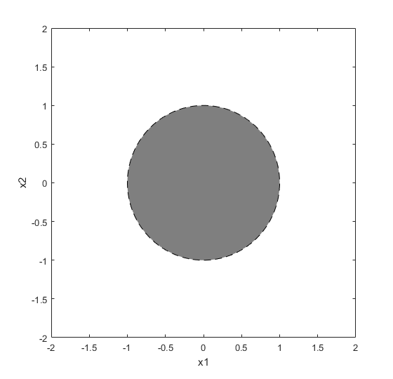
Unlike the above example, $LM_{p}$ (or even $\overline{LM_{p}}$ as $LM_{p}$ is in general not closed) may not be a polyhedral⁵⁵ 5 Recall that a polyhedron is a set defined by finitely many affine inequalities. set for cubic polynomials. For instance, the polynomial

p(x_{1},x_{2},x_{3},x_{4})=-x_{1}x_{3}^{2}+x_{1}x_{4}^{2}+2x_{2}x_{3}x_{4}+x_{3}^{2}+x_{4}^{2},

(10)

has $LM_{p}=\{x\in\mathbb{R}^{4}\ |\ x_{1}^{2}+x_{2}^{2}<1,x_{3}=x_{4}=0\}$ (see Figure 3). This is in contrast to quadratic polynomials, whose local minima always form a polyhedral set. We show in Theorem 4.5, however, that $\overline{LM_{p}}$ is always a spectrahedron⁶⁶ 6 Recall that a spectrahedron is a set of the type $S=\{x\in\mathbb{R}^{n}|A_{0}+\sum_{i=1}^{n}x_{i}A_{i}\succeq 0\}$ , where $A_{0},\ldots A_{n}$ are symmetric matrices of some size $m\times m$ [30].. We first need the following lemma.

For any cubic polynomial $p:\mathbb{R}^{n}\to\mathbb{R}$ , suppose $\bar{x}\in\mathbb{R}^{n}$ and $\bar{y}\in\mathbb{R}^{n}$ satisfy

•

$\bar{x}\in SO_{p}$ ,
•

$\nabla^{2}p(\bar{y})\succeq 0$ ,
•

$p(\bar{x})=p(\bar{y})$ .

Then $p(\bar{x}+\alpha(\bar{y}-\bar{x}))=p(\bar{x})$ for any scalar $\alpha$ , and $\bar{y}-\bar{x}\in\mathcal{N}(\nabla^{2}p(\bar{x}))$ .

Note in particular that this lemma applies if $\bar{y}$ is simply a second-order point, since $p$ must take the same value at any two second-order points. This is because any non-constant univariate cubic polynomial can have at most one second-order point.

Consider the Taylor expansion of $p$ around $\bar{x}$ in the direction $\bar{y}-\bar{x}$ (see (2)):

q(\alpha)\mathrel{\mathop{:}}=p(\bar{x}+\alpha(\bar{y}-\bar{x}))=p_{3}(\bar{y}-\bar{x})\alpha^{3}+\frac{1}{2}(\bar{y}-\bar{x})^{T}\nabla^{2}p(\bar{x})(\bar{y}-\bar{x})\alpha^{2}+\nabla p(\bar{x})^{T}(\bar{y}-\bar{x})\alpha+p(\bar{x}).

Note that $q$ is a univariate cubic polynomial which has a second-order point at $\alpha=0$ . It is straightforward to see that if a univariate cubic polynomial is not constant and has a second-order point, then any other point which takes the same function value as the second-order point must have a negative second derivative. As this is not the case for $q$ (in view of $\alpha=0$ and $\alpha=1$ ), $q$ must be constant, i.e., $p(\bar{x}+\alpha(\bar{y}-\bar{x}))=p(\bar{x})$ for any $\alpha$ . Now observe that for $p(\bar{x}+\alpha(\bar{y}-\bar{x}))$ to be constant, we must have $(\bar{y}-\bar{x})^{T}\nabla^{2}p(\bar{x})(\bar{y}-\bar{x})=0$ . As $\nabla^{2}p(\bar{x})\succeq 0$ , we have $\bar{y}-\bar{x}\in\mathcal{N}(\nabla^{2}p(\bar{x}))$ . ∎

For a cubic polynomial $p:\mathbb{R}^{n}\to\mathbb{R},\overline{LM_{p}}$ is a spectrahedron.

If $LM_{p}$ is empty, the claim is trivial. Otherwise, let $\bar{x}\in LM_{p}$ . We show that $\overline{LM_{p}}$ is given by the spectrahedron

M\mathrel{\mathop{:}}=\{x\in\mathbb{R}^{n}\ |\ \nabla^{2}p(x)\succeq 0,\nabla^{2}p(\bar{x})(x-\bar{x})=0\}.

(11)

First consider any $\bar{y}\in LM_{p}$ . From the SONC we know that $\nabla^{2}p(\bar{y})\succeq 0$ and from Lemma 4.4, we know that $\bar{y}-\bar{x}\in\mathcal{N}(\nabla^{2}p(\bar{x}))$ . Thus $\bar{y}\in M$ . Since $M$ is closed, we get that $\overline{LM_{p}}\subseteq M$ .

Now consider any $\bar{y}\in M$ . By the definition of $M$ , $\bar{y}$ satisfies the SONC, and by Lemma 4.2, it also satisfies the FONC. Since for any scalar $\alpha\in(0,1)$ , $\nabla^{2}p(\bar{x}+\alpha(\bar{y}-\bar{x}))$ is a convex combination of the two psd matrices $\nabla^{2}p(\bar{x})$ and $\nabla^{2}p(\bar{y})$ , we have $\mathcal{N}(\nabla^{2}p(\bar{x}+\alpha(\bar{y}-\bar{x})))\subseteq\nabla^{2}p(\bar{x})$ and thus $\bar{x}+\alpha(\bar{y}-\bar{x})$ satisfies the TOC (since $\bar{x}$ does). Thus $\bar{y}$ can be written as the limit of local minima of $p$ (e.g. $\{\bar{x}+\alpha(\bar{y}-\bar{x})\}$ as $\alpha\to 1$ ). ∎

We will soon show that for a cubic polynomial $p$ , if $LM_{p}$ is nonempty, then $\overline{LM_{p}}=SO_{p}$ (see Theorem 4.7). In Section 6, we will give other representations of $SO_{p}$ , which in contrast to the representation in (11), do not rely on access to or even existence of a local minimum.

In Section 6, we present an SDP-based approach for finding local minima of cubic polynomials. (We note again that the SDP representation in (11) is useless for this purpose as it already assumes access to a local minimum.) Many common approaches for computing local minima of twice-differentiable functions involve first finding critical points of the function, and then checking whether they satisfy second-order conditions. However, as discussed in the introduction and in Section 2, such approaches are unlikely to be effective for cubic polynomials as critical points of these functions are in fact NP-hard to find (see Theorem 2.1). Interestingly, however, we show in Section 6 that by bypassing the search for critical points, one can directly find second-order points and local minima of cubic polynomials by solving semidefinite programs of tractable size. The key to our approach is to relate the problem of finding a local minimum of a cubic polynomial $p$ to the following optimization problem:

		$\displaystyle\underset{x\in\mathbb{R}^{n}}{\inf}$		$\displaystyle p(x)$		(12)
		$\displaystyle\text{subject to}$		$\displaystyle\nabla^{2}p(x)\succeq 0.$		(12)

The connection between solutions of (12) and local minima of $p$ is established by Theorem 4.7 below. The feasible set of (12) has interesting geometric properties (see, e.g., Corollary 4.12) and will be referred to with the following terminology in the remainder of the paper.

The convexity region of a polynomial $p:\mathbb{R}^{n}\to\mathbb{R}$ is the set

CR_{p}\mathrel{\mathop{:}}=\{x\in\mathbb{R}^{n}\ |\ \nabla^{2}p(x)\succeq 0\}.

Observe that for any cubic polynomial, its convexity region is a spectrahedron, and thus a convex set. As $p$ is a convex function when restricted to its convexity region, one can consider (12) to be a convex problem in spirit.

Let $p$ be a cubic polynomial with a second-order point. Then the following sets are equivalent:

(i)

$SO_{p}$
(ii)

Minima of (12).

Furthermore, if $p$ has a local minimum, then these two sets are equivalent to:

(iii)

$\overline{LM_{p}}$ .

$(i)\subseteq(ii)$ .
Let $\bar{y}\in SO_{p}$ and $\bar{x}$ be any feasible point to (12). If we consider the univariate cubic polynomial $q(\alpha)\mathrel{\mathop{:}}=p(\bar{x}+\alpha(\bar{y}-\bar{x}))$ , i.e., the restriction of $p$ to the line passing through $\bar{x}$ and $\bar{y}$ , we can see that $\alpha=1$ is a second-order point of $q$ . Note that if any univariate cubic polynomial has a second-order point, then that second-order point is a minimum of it over its convexity region. In particular, because $\bar{x}$ is feasible to (12) and thus $\alpha=0$ is in the convexity region of $q$ , we have $p(\bar{y})=q(1)\leq q(0)=p(\bar{x})$ . As $\bar{y}$ is feasible to (12) and has objective value no higher than any other feasible point, it must be optimal to (12).

$(ii)\subseteq(i)$
Let $\bar{y}$ be a minimum of (12) (we know that such a point exists because we have shown $SO_{p}$ is a subset of the minima of (12), and $SO_{p}$ is nonempty by assumption). Let $\bar{x}\in SO_{p}$ and $d\mathrel{\mathop{:}}=\bar{y}-\bar{x}$ . Observe that $p(\bar{y})=p(\bar{x})$ , and so by Lemma 4.4, we must have $d\in\mathcal{N}(\nabla^{2}p(\bar{x}))$ . It follows that $\nabla p(\bar{y})=\nabla p_{3}(d)$ (cf. the proof of Lemma 4.2). Now suppose for the sake of contradiction that $\bar{y}$ is not a second-order point. Since $\bar{y}$ is feasible to (12), we must have $\nabla p(\bar{y})=\nabla p_{3}(d)\neq 0$ . As $p(\bar{x})=p(\bar{x}+\alpha d)$ for any scalar $\alpha$ due to Lemma 4.4, we must have $p_{3}(d)=\frac{1}{6}d^{T}\nabla^{2}p_{3}(d)d=0$ (see (2)). Thus we can write

	$\displaystyle\big(d-\alpha\nabla p_{3}(d)\big)^{T}\nabla^{2}p(\bar{y})\big(d-\alpha\nabla p_{3}(d)\big)=$	$\displaystyle\big(d-\alpha\nabla p_{3}(d)\big)^{T}\big(\nabla^{2}p(\bar{x})+\nabla^{2}p_{3}(d)\big)\big(d-\alpha\nabla p_{3}(d)\big)$
	$\displaystyle=$	$\displaystyle\alpha^{2}\nabla p_{3}(d)^{T}\nabla^{2}p(\bar{x})\nabla p_{3}(d)-2\alpha\nabla p_{3}(d)^{T}\nabla^{2}p_{3}(d)^{T}d$
		$\displaystyle+\alpha^{2}\nabla p_{3}(d)^{T}\nabla^{2}p_{3}(d)\nabla p_{3}(d)$
	$\displaystyle=$	$\displaystyle\alpha^{2}\left(\nabla p_{3}(d)^{T}\nabla^{2}p(\bar{x})\nabla p_{3}(d)+\nabla p_{3}(d)^{T}\nabla^{2}p_{3}(d)^{T}\nabla p_{3}(d)\right)$
		$\displaystyle-4\alpha\nabla p_{3}(d)^{T}\nabla p_{3}(d),$

where the last equality follows from that $\nabla p_{3}(d)=\frac{1}{2}\nabla^{2}p_{3}(d)^{T}d$ due to Euler’s theorem for homogeneous functions. Note that the right-hand side of the above expression is negative for sufficiently small $\alpha>0$ , and so $\nabla^{2}p(\bar{y})$ is not psd, which contradicts feasibility of $\bar{y}$ to (12).

For the second claim of the theorem, suppose that $p$ has a local minimum. The following arguments will show $(i)=(ii)=(iii).$

$(iii)\subseteq(i)$
Clearly any local minimum of $p$ is a second-order point. Since the gradient and the Hessian of $p$ are continuous in $x$ and as the cone of psd matrices is closed, the limit of any convergent sequence of second-order points is a second-order point.

$(ii)\subseteq(iii)$ .
Let $\bar{y}$ be any minimum of (12). Consider any local minimum $\bar{x}$ of $p$ and let $z_{\alpha}\mathrel{\mathop{:}}=\bar{x}+\alpha(\bar{y}-\bar{x})$ . As both $\nabla^{2}p(\bar{y})$ and $\nabla^{2}p(\bar{x})$ are psd, any point $z_{\alpha}$ with $\alpha\in[0,1)$ satisfies the SONC and TOC, by the same arguments as in the proof of Theorem 4.3. Now note that since $\bar{x}$ is a second-order point, it is also a minimum of (12) (as $(i)\subseteq(ii)$ ) and thus $p(\bar{y})=p(\bar{x})$ . From Lemma 4.4, we then have $\bar{y}-\bar{x}\in\mathcal{N}(\nabla^{2}p(\bar{x}))$ , and so from Lemma 4.2, $z_{\alpha}$ satisfies the FONC for any $\alpha$ . Thus, in view of Theorem 3.1, for any $\alpha\in[0,1),z_{\alpha}$ is a local minimum of $p$ . Therefore $\bar{y}$ can be written as the limit of a sequence of local minima (i.e., $\{z_{\alpha}\}$ as $\alpha\to 1$ ), and hence $\bar{y}\in\overline{LM_{p}}$ . ∎

Note that as a consequence of Theorems 4.5 and 4.7, if a cubic polynomial $p$ has a local minimum, then $SO_{p}$ is a spectrahedron. In fact, $SO_{p}$ is a spectrahedron for any cubic polynomial $p$ ; see Theorem 6.3. In that theorem, we will give a more useful spectrahedral representation of $SO_{p}$ which does not rely on knowledge of a local minimum.

Let $p$ be a cubic polynomial with a second-order point. Then the optimal value of (12) is the value that $p$ takes at any of its second-order points (and in particular, at any of its local minima if they exist).

This is immediate from the equivalence of $(i)$ and $(ii)$ in Theorem 4.7. ∎

We have shown that the optimization problem in (12) gives an approach for finding second-order points of a cubic polynomial $p$ without computing its critical points. However, not all second-order points are local minima, and so in this subsection, we characterize the difference between the two notions more precisely. We first recall the concept of the relative interior of a (convex) set (see, e.g., [26, Chap. 6]).

The relative interior of a nonempty convex set $S\subseteq\mathbb{R}^{n}$ is the set

ri(S)\mathrel{\mathop{:}}=\{x\in S\ |\ \forall y\in S,\exists\lambda>1\ s.t.\ \lambda x+(1-\lambda)y\in S\}.

This definition generalizes the notion of interior to sets which do not have full dimension. One can show that for a convex set $S$ , $ri(S)$ is convex, $ri(\bar{S})=ri(S)$ , and $\overline{ri(S)}=\bar{S}$ [26]. In general, for a nonempty convex set $S$ , we have $ri(\bar{S})=ri(S)\subseteq S$ , but we may not have $ri(\bar{S})=S$ . (For example, let $S$ be a line segment with one of its endpoints removed.) It turns out, however, that for a cubic polynomial $p$ with a local minimum, $ri(\overline{LM_{p}})=LM_{p}$ .

Let $p:\mathbb{R}^{n}\to\mathbb{R}$ be a cubic polynomial with a local minimum. Then the following three sets are equivalent:

(i)

$LM_{p}$
(ii)

$ri(SO_{p})$
(iii)

Intersection of critical points of $p$ with $ri(CR_{p})$ .

$(ii)\subseteq(i)$
Recall from Theorem 4.3 that $LM_{p}$ is convex, and from Theorem 4.7 that $SO_{p}=\overline{LM_{p}}$ . Then we have $ri(SO_{p})=ri(\overline{LM_{p}})=ri(LM_{p})\subseteq LM_{p}$ .

$(i)\subseteq(ii)$
We prove the contrapositive. Let $\bar{x}$ be a point which is not in $ri(SO_{p})$ . If $\bar{x}$ is not a second-order point, then it clearly cannot be a local minimum. Suppose now that $\bar{x}\in SO_{p}\backslash ri(SO_{p})$ . Then there is another second-order point $\bar{y}$ such that $\bar{y}+\lambda(\bar{x}-\bar{y})$ is not a second-order point for any $\lambda>1$ . Note from Lemma 4.4 and the statement after it that $p(\bar{y}+\lambda(\bar{x}-\bar{y}))$ is a constant univariate function of $\lambda$ . Now for any $\epsilon>0$ , define the point $\bar{z}_{\epsilon}\mathrel{\mathop{:}}=\bar{x}+\frac{\epsilon}{2\|\bar{x}-\bar{y}\|}(\bar{x}-\bar{y})$ . Since $\bar{z}_{\epsilon}$ is not a second-order point and thus not a local minimum, there is a point $z_{\epsilon}$ satisfying $\|\bar{z}_{\epsilon}-z_{\epsilon}\|<\frac{\epsilon}{2}$ and

p(z_{\epsilon})<p(\bar{z}_{\epsilon})=p(\frac{\epsilon}{2\|\bar{x}-\bar{y}\|}(\bar{x}-\bar{y}))=p(\bar{x}).

Furthermore, by the triangle inequality, $z_{\epsilon}$ also satisfies $\|z_{\epsilon}-\bar{x}\|<\epsilon$ . Thus, by considering $\{z_{\epsilon}\}$ as $\epsilon\to 0$ , we can conclude that $\bar{x}$ is not a local minimum.

$(i)\subseteq(iii)$
Consider any local minimum $\bar{x}$ of $p$ , which clearly must also be a critical point of $p$ , and a member of $CR_{p}$ . Suppose for the sake of contradiction that $\bar{x}\not\in ri(CR_{p})$ . Then there exists $y\in CR_{p}$ such that for any scalar $\alpha>0,\nabla^{2}p(\bar{x}+\alpha(\bar{x}-y))$ is not psd. In particular, for any $\alpha>0$ there exists a unit vector $z_{\alpha}\in\mathbb{R}^{n}$ such that $z_{\alpha}^{T}\nabla^{2}p(\bar{x}+\alpha(\bar{x}-y))z_{\alpha}<0$ .

We now show that for any $\alpha$ , $z_{\alpha}$ can be taken to be in $\mathcal{C}(\nabla^{2}p(\bar{x}))$ . This is because, as we will show, if $z_{\alpha}=d+v$ , where $d\in\mathcal{N}(\nabla^{2}p(\bar{x}))$ and $v\in\mathcal{C}(\nabla^{2}p(\bar{x}))$ ,

(d+v)^{T}\nabla^{2}p(\bar{x}+\alpha(\bar{x}-y))(d+v)=v^{T}\nabla^{2}p(\bar{x}+\alpha(\bar{x}-y))v.

(13)

Observe that if $p$ is written in the form (4), for any $d~\in~\mathcal{N}(\nabla^{2}p(\bar{x}))$ , we have

	$\displaystyle d^{T}\nabla^{2}p(\bar{x}+\alpha(\bar{x}-y))d$	$\displaystyle=d^{T}\left(\sum_{i=1}^{n}(\bar{x}_{i}+\alpha(\bar{x}_{i}-y_{i}))H_{i}+Q\right)d$
		$\displaystyle=d^{T}\left(\sum_{i=1}^{n}\bar{x}_{i}H_{i}+Q\right)d+\alpha\sum_{i=1}^{n}(d^{T}H_{i}d)(\bar{x}_{i}-y_{i})=0,$

where the last equality follows from that $d\in\mathcal{N}(\nabla^{2}p(\bar{x}))$ , and the TOC, recalling that the $i$ -th entry of $\nabla p_{3}(d)$ is $\frac{1}{2}d^{T}H_{i}d$ . Note in particular that the expression above also holds for $\alpha=-1$ , and so $d\in\mathcal{N}(\nabla^{2}p(y))$ . Now observe that because we can write

\nabla^{2}p(\bar{x}+\alpha(\bar{x}-y))=(1+\alpha)\nabla^{2}p(\bar{x})-\alpha\nabla^{2}p(y),

we have $\nabla^{2}p(\bar{x}+\alpha(\bar{x}-y))d=0$ . Thus, we have shown (13), and we can take $z_{\alpha}\in\mathcal{C}(\nabla^{2}p(\bar{x}))$ .

Note that if $z_{\alpha}\in\mathcal{C}(\nabla^{2}p(\bar{x}))$ , then by Lemma 3.2 we have $z_{\alpha}^{T}\nabla^{2}p(\bar{x})z_{\alpha}\geq\lambda$ , where $\lambda$ is the smallest nonzero eigenvalue of $\nabla^{2}p(\bar{x})$ . Thus, for small enough $\alpha$ , the quantity $z_{\alpha}^{T}\nabla^{2}p(\bar{x}+\alpha(\bar{x}-y))z_{\alpha}$ is positive and so we arrive at a contradiction.

$(iii)\subseteq(i)$
Let $\bar{x}$ be a critical point which is in $ri(CR_{p})$ . Clearly $\bar{x}\in SO_{p}$ . Consider any local minimum $\bar{y}$ of $p$ , and observe that for any $\alpha\neq 0$ , we can write

\bar{x}=\frac{1}{\alpha}(\alpha\bar{x}+(1-\alpha)\bar{y})+\frac{\alpha-1}{\alpha}\bar{y}.

(14)

As $\bar{x}\in ri(CR_{p})$ and $\bar{y}\in CR_{p},\alpha\bar{x}+(1-\alpha)\bar{y}\in CR_{p}$ for some $\alpha>1$ . In particular, for that $\alpha,\nabla^{2}p(\alpha\bar{x}+(1-\alpha)\bar{y})\succeq 0$ and thus in view of (14), we can see that $\mathcal{N}(\nabla^{2}p(\bar{x}))\subseteq\mathcal{N}(\nabla^{2}p(\bar{y}))$ . Hence, because the TOC holds at $\bar{y}$ , it must also hold at $\bar{x}$ . Thus $\bar{x}$ is a local minimum. ∎

Figure 4 demonstrates the relation between $LM_{p}$ and $SO_{p}$ for the polynomial $p(x_{1},x_{2})=x_{1}^{2}x_{2}$ . For this example, $SO_{p}=\{(x_{1},x_{2})\ |\ x_{1}=0,x_{2}\geq 0\}$ , and $LM_{p}=\{(x_{1},x_{2})\ |\ x_{1}=0,x_{2}>0\}$ (see Example 3.1).

Theorem 4.10 gives rise to the following interesting geometric fact about local minima of cubic polynomials.

Let $\bar{x}$ and $\bar{y}$ be two local minima of a cubic polynomial. Then

\mathcal{N}(\nabla^{2}p(\bar{x}))=\mathcal{N}(\nabla^{2}p(\bar{y})).

It is known (see [25, Corollary 1]) that for a spectrahedron $\{x\in\mathbb{R}^{n}\ |\ A_{0}+\sum_{i=1}^{n}x_{i}A_{i}\succeq 0\}$ and any two points $x$ and $y$ in its relative interior, $\mathcal{N}(A_{0}+\sum_{i=1}^{n}x_{i}A_{i})=\mathcal{N}(A_{0}+\sum_{i=1}^{n}y_{i}A_{i})$ . In view of the facts that for any cubic polynomial $p$ , $CR_{p}$ is a spectrahedron and $LM_{p}\subseteq ri(CR_{p})$ (from Theorem 4.10), the result is immediate. ∎

We end this section with a result relating general spectrahedra and convexity regions of cubic polynomials. Recall from the end of Section 3.1 that if $S\mathrel{\mathop{:}}=\{x\in\mathbb{R}^{n}\ |\ A_{0}+\sum_{i=1}^{n}x_{i}A_{i}\succeq 0\}$ is a special spectrahedron, where $A_{0},\ldots,A_{n}$ are $n\times n$ symmetric matrices satisfying

(A_{i})_{jk}=(A_{j})_{ik}=(A_{k})_{ij}

for any $i,j,k\in\{1,\ldots,n\}$ , then $S$ is the convexity region of the cubic polynomial

p(x)=\frac{1}{6}\sum_{i=1}^{n}x^{T}x_{i}A_{i}x+\frac{1}{2}x^{T}A_{0}x.

The following theorem shows that if the number of variables is allowed to increase, then any spectrahedron can be represented by the convexity region of a cubic polynomial.

Let a spectrahedron $S\subseteq\mathbb{R}^{n}$ be given by $S\mathrel{\mathop{:}}=\{x\in\mathbb{R}^{n}\ |\ A_{0}+\sum_{i=1}^{n}x_{i}A_{i}\succeq 0\}$ , where $A_{0},\ldots,A_{n}\in\mathbb{S}^{m\times m}$ . There exists a cubic polynomial $p$ in at most $m+n$ variables such that $S$ is a projection of its convexity region; i.e.,

S=\{x\in\mathbb{R}^{n}\ |\ \exists y\in\mathbb{R}^{m}\mbox{ such that }(x,y)\in CR_{p}\}.

Furthermore, the interior of $S$ is a projection of the set of local minima of $p$ .

Let $A(x)\mathrel{\mathop{:}}=A_{0}+\sum_{i=1}^{n}x_{i}A_{i}$ . We first present a characterization of the interior of $S$ following the developments in Section 2.4 of [25]. Let $\mathcal{N}_{A}\mathrel{\mathop{:}}=\mathcal{N}(A_{0})\cap\ldots\cap\mathcal{N}(A_{n})$ , and $V$ be a full-rank matrix whose columns span the orthogonal complement of $\mathcal{N}_{A}$ . Suppose that $\mathcal{N}_{A}$ is $(m-k)$ -dimensional. Then there exist matrices $B_{0},\ldots,B_{n}\in\mathbb{S}^{k\times k}$ with $\mathcal{N}(B_{0})\cap\ldots\cap\mathcal{N}(B_{n})=\{0_{k}\}$ such that

B(x)\mathrel{\mathop{:}}=B_{0}+\sum_{i=1}^{n}x_{i}B_{i}=V^{T}A(x)V.

In [25, Corollary 5], it is shown that $B(x)$

\{x\in\mathbb{R}^{n}\ |\ A(x)\succeq 0\}=\{x\in\mathbb{R}^{n}\ |\ B(x)\succeq 0\}

(15)

and that the set $\{x\in\mathbb{R}^{n}\ |\ B(x)\succ 0\}$ gives the interior of $S$ . Now consider the following cubic polynomial in $n+k$ variables:

p(x,y)\mathrel{\mathop{:}}=y^{T}B(x)y.

(16)

Observe that the partial derivative of $p$ with respect to $y$ is $2B(x)y$ , the partial derivative of $p$ with respect to $x_{i}$ is $y^{T}B_{i}y$ , and the Hessian of $p$ is

\nabla^{2}p(x,y)=2\left[\begin{matrix}0&C(y)^{T}\\ C(y)&B(x)\end{matrix}\right],

where $C(y)$ is an $k\times n$ matrix whose $i$ -th column equals $B_{i}y$ . One can then immediately see that if $(\bar{x},\bar{y})\in CR_{p}$ , then we must have $B(\bar{x})\succeq 0$ . Conversely, if $B(\bar{x})\succeq 0$ , then $(\bar{x},0_{k})\in CR_{p}$ . Hence, in view of (15), we have shown that the spectrahedron $S$ is the projection of $CR_{p}$ onto the $x$ variables.

We now show that $LM_{p}=\{x\in\mathbb{R}^{n}\ |\ B(x)\succ 0\}\times\{0_{k}\}$ . This would prove the second claim of the theorem. First let $\bar{x}$ be such that $B(\bar{x})\succ 0$ . Note that $p(\bar{x},0_{k})=0$ and that for any two vectors $\chi\in\mathbb{R}^{n}$ and $\psi\in\mathbb{R}^{k}$ ,

p(\bar{x}+\chi,\psi)=\psi^{T}\left(B(\bar{x})+\sum_{i=1}^{n}B_{i}\chi_{i}\right)\psi.

Since $B(\bar{x})\succ 0$ , then for any $\chi$ of sufficiently small norm, $B(\bar{x})+\sum_{i=1}^{n}B_{i}\chi_{i}$ is still positive definite, and hence for any $\psi$ , $p(\bar{x}+\chi,\psi)\geq 0=p(\bar{x},0_{k})$ . Thus $(\bar{x},0_{k})$ is a local minimum of $p$ .

Now let $(\bar{x},\bar{y})$ be a local minimum of $p$ . From the SONC, we must have $B(\bar{x})\succeq 0$ and $C(\bar{y})=0$ , which implies that $B_{i}\bar{y}=0_{k},\forall i\in\{1,\ldots,n\}$ . Since

\frac{\partial p}{\partial y}(\bar{x},\bar{y})=2B(\bar{x})\bar{y}=2\left(B_{0}+\sum_{i=1}^{n}\bar{x}_{i}B_{i}\right)\bar{y}=2B_{0}\bar{y}+2\sum_{i=1}^{n}\bar{x}_{i}(B_{i}\bar{y}),

it further follows from the FONC that $B_{0}\bar{y}=0$ . As $\mathcal{N}(B_{0})\cap\ldots\cap\mathcal{N}(B_{n})=\{0_{k}\}$ by construction, it follows that we must have $\bar{y}=0_{k}$ . Next, observe that $\mathcal{N}(\nabla^{2}p(\bar{x},0_{k}))=\mathbb{R}^{n}\times\mathcal{N}(B(\bar{x}))$ . Let $d\in\mathcal{N}(B(\bar{x}))$ , and note that for any $i\in\{1,\ldots,n\}$ , $(e_{i},d)\in\mathcal{N}(\nabla^{2}p(\bar{x},0_{k}))$ and $\frac{\partial p_{3}}{\partial y}(e_{i},d)=B_{i}d$ . Then from the TOC, we must have $B_{i}d=0_{k},\forall i\in\{1,\ldots,n\}$ . Furthermore, since $d\in\mathcal{N}(B(\bar{x}))$ , it follows that $B_{0}d=0_{k}$ as well. Again, as $\mathcal{N}(B_{0})\cap\ldots\cap\mathcal{N}(B_{n})=\{0_{k}\}$ by construction, it follows that we must have $d=0_{k}$ and thus $B(\bar{x})\succ 0$ . ∎

In the next section, we show that second-order points and local minima of cubic polynomials can be found by solving polynomially-many semidefinite programs with a polynomial number of variables and constraints. One caveat however is that the inputs and outputs of these semidefinite programs can sometimes be algebraic but not necessarily rational numbers. As a result, we cannot claim that second-order points and local minima of cubic polynomials can be found in polynomial time in the Turing model of computation. In this subsection, we give evidence as to why establishing the complexity of these problems in the Turing model is at the moment likely out of reach.

The SDP Feasibility Problem (SDPF) is the following decision question: Given $m\times m$ symmetric matrices $A_{0},\ldots,A_{n}$ with rational entries, decide whether there exists a vector $x\in\mathbb{R}^{n}$ such that $A_{0}+\sum_{i=1}^{n}x_{i}A_{i}\succeq 0$ .

The SDP Strict Feasibility Problem (SDPSF) is the following decision question: Given $m\times m$ symmetric matrices $A_{0},\ldots,A_{n}$ with rational entries, decide whether there exists a vector $x\in\mathbb{R}^{n}$ such that $A_{0}+\sum_{i=1}^{n}x_{i}A_{i}\succ 0$ .

Even though semidefinite programs can be solved to arbitrary accuracy in polynomial time [29], the complexities of the decision problems above remain as two of the outstanding open problems in semidefinite programming. At the moment, it is not known if these two decision problems even belong to the class NP [23, 22, 7]. We show next that the complexities of these problems are a lower bound on the complexities of testing existence of second-order points and local minima of cubic polynomials. (In Section 6, we accomplish the more involved task of giving the reduction in the opposite direction.)

If the problem of deciding whether a cubic polynomial has any second-order points is in P (resp. NP), then SDPF is in P (resp. NP).

Given matrices $A_{0},\ldots,A_{n}\in\mathbb{S}^{m\times m}$ , let $A(x)\mathrel{\mathop{:}}=A_{0}+\sum_{i=1}^{n}x_{i}A_{i}$ . By noting that the cubic polynomial $p(x,y)=y^{T}A(x)y$ has as its Hessian

\nabla^{2}p(x,y)=2\left[\begin{matrix}0&B(y)^{T}\\ B(y)&A(x)\end{matrix}\right],

where $B(y)$ is an $m\times n$ matrix whose $i$ -th column equals $A_{i}y$ , we can see that if $A(\bar{x})\succeq 0$ for some $\bar{x}\in\mathbb{R}^{n}$ , then $\nabla^{2}p(\bar{x},0_{k})\succeq 0$ . Since $p$ is quadratic in the variables $y$ , $\nabla p(\bar{x},0_{k})=0_{m+n}$ , and hence $(\bar{x},0_{k})$ is a second-order point of $p$ . Conversely, if $A(x)\not\succeq 0$ for any $x\in\mathbb{R}^{n}$ , then clearly $\nabla^{2}p(x,y)\not\succeq 0$ for any $x\in\mathbb{R}^{n}$ and $y\in\mathbb{R}^{m}$ , and thus $p$ cannot have any second-order points.

The above reduction shows that any polynomial-time algorithm (or polynomial-time verifiable certificate) for existence of second-order points of cubic polynomials translates into one for SDPF. ∎

If the problem of deciding whether a cubic polynomial has any local minima is in P (resp. NP), then SDPSF is in P (resp. NP).

Given matrices $A_{0},\ldots,A_{n}\in\mathbb{S}^{m\times m}$ , let $A(x)\mathrel{\mathop{:}}=A_{0}+\sum_{i=1}^{n}x_{i}A_{i}$ and consider the set $S\mathrel{\mathop{:}}=\{x\in\mathbb{R}^{n}\ |\ A(x)\succeq 0\}$ . It is not difficult to see that there exists $\bar{x}\in\mathbb{R}^{n}$ such that $A(\bar{x})\succ 0$ if and only if $S$ has a nonempty interior and $\mathcal{N}_{A}\mathrel{\mathop{:}}=\mathcal{N}(A_{0})\cap\mathcal{N}(A_{1})\cap\mathcal{N}(A_{2})\ldots\cap\mathcal{N}(A_{n})=\{0_{m}\}$ .⁷⁷ 7 The “only if” direction is straightforward and the “if” direction follows from [25, Corollary 5]. The latter condition can be checked in polynomial time by solving linear systems. The former can be reduced—due to the second claim of Theorem 4.12—to deciding if the cubic polynomial constructed in (16) has a local minimum. Note that the polynomial in (16) has coefficients polynomially sized in the entries of the matrices $A_{i}$ , since the matrix $V$ in the proof of Theorem 4.12 can be taken to be the identity matrix when $\mathcal{N}_{A}=\{0_{m}\}$ . ∎

In addition to the difficulties alluded to in the above two theorems, the following three examples point to concrete representation issues that one encounters in the Turing model when dealing with local minima of cubic polynomials. The same complications are known to arise for SDP feasibility problems [7].

A cubic polynomial with only irrational local minima. Consider the univariate cubic polynomial $p(x)=x^{3}-6x$ . One can easily verify that its unique local minimum is at $x=\sqrt{2},$ which is irrational even though the coefficients of $p$ are rational.

A cubic polynomial with an irrational convexity region. Consider the quintary cubic polynomial $p(x,y)=y^{T}A(x)y$ , where

A(x)=\left[\begin{matrix}2&x&0&0\\ x&1&0&0\\ 0&0&2x&2\\ 0&0&2&x\end{matrix}\right].

One can easily verify that $x=\sqrt{2}$ is the only scalar satisfying $A(x)\succeq 0$ . Since the matrix $2A(x)$ is a principal submatrix of $\nabla^{2}p(x,y)$ , any point in the convexity region of $p$ must satisfy $x=\sqrt{2}$ (even though the coefficients of $p$ are rational).

A family of cubic polynomials whose local minima have exponential bitsize. Consider the family of cubic polynomials $p_{n}(x,y)=y^{T}A_{n}(x)y$ in $3n$ variables, where

A_{n}(x)=\left[\begin{matrix}x_{1}&2&0&0&\cdots&0&0\\ 2&1&0&0&\cdots&0&0\\ 0&0&x_{2}&x_{1}&\cdots&0&0\\ 0&0&x_{1}&1&\cdots&0&0\\ \cdots&\cdots&\cdots&\cdots&\ddots&\cdots&\cdots\\ 0&0&0&0&\cdots&x_{n}&x_{n-1}\\ 0&0&0&0&\cdots&x_{n-1}&1\end{matrix}\right].

We show that even though these polynomials have some rational local minima, it takes exponential time to write them down. From the proof of Theorem 4.12, one can infer that the set of local minima of $p_{n}$ is the set $\{x\in\mathbb{R}^{n}\ |\ A_{n}(x)\succ 0\}\times\{0_{2n}\}$ . However, observe that to have $A_{n}(x)\succ 0$ (or even $A_{n}(x)\succeq 0)$ , we must have

x_{1}\geq 4,x_{2}\geq 16,\ldots,x_{n}\geq 2^{2^{n}}.

Hence, any local minimum of $p_{n}$ has bit length at least $O(2^{n})$ even though the bit length of the coefficients of $p_{n}$ is $O(n)$ .

In this section, we derive an SDP-based approach for finding second-order points and local minima of cubic polynomials. This, along with the results established in Section 2, will complete the entries of Table 2 from Section 1. We begin with some preliminaries that are needed to present the theorems of this section.

Recall that a spectrahedron is a set of the type

\left\{x\in\mathbb{R}^{n}\ |\ A_{0}+\sum_{i=1}^{n}x_{i}A_{i}\succeq 0\right\},

where $A_{0},\ldots,A_{n}$ are symmetric matrices of some size $m\times m$ . A semidefinite representable set (also known as a spectrahedral shadow) is a set of the type

\left\{x\in\mathbb{R}^{n}\ |\ \exists y\in\mathbb{R}^{k}\text{ such that }A_{0}+\sum_{i=1}^{n}x_{i}A_{i}+\sum_{i=1}^{k}y_{i}B_{i}\succeq 0\right\},

(17)

for some integer $k\geq 0$ and symmetric $m\times m$ matrices $A_{0},A_{1},\ldots,A_{n},B_{1},\ldots,B_{k}$ . These are exactly sets which semidefinite programming can optimize over.

We show in Theorem 6.3 and Corollary 6.5 that the set of second-order points of any cubic polynomial is a spectrahedron and describe how a description of this spectrahedron can be obtained from the coefficients of $p$ only.⁸⁸ 8 Recall that the results of Section 4 by contrast established spectrahedrality of the set of second-order points under the assumption of existence of a local minimum (see Remark 4.2). Furthermore, the spectrahedral representation that we gave there (see Theorem 4.5) required knowledge of a local minimum. Since relative interiors of semidefinite representable sets (and in particular spectrahedra) are semidefinite representable [19, Theorem 3.8], it follows from our Theorem 4.10 that the set of local minima of any cubic polynomial is semidefinite representable.

Due to the complexity results and representation issues presented in Section 5, we assume in this section that we can do arithmetic over real numbers and have access to an oracle which solves SDPs exactly. This oracle—which we call E-SDP---takes as input an SDP with real data and outputs the optimal value as a real number if it is finite, or reports that the SDP is infeasible, or that it is unbounded.⁹⁹ 9 Though this will not be needed for our purposes, it is straightforward to show that for an SDP with $n$ scalar variables, the oracle E-SDP can be called twice to test attainment of the optimal value, and a total of $n+1$ times to recover an optimal solution. The following lemma shows that E-SDP can find a point in the relative interior of a semidefinite representable set. This will be relevant for us later in this section when we search for local minima of cubic polynomials.

Let $S$ be a nonempty semidefinite representable set in $\mathbb{R}^{n}$ . Then a point in $ri(S)$ can be recovered in $2n$ calls to E-SDP.

Consider the following procedure. Let $S_{1}=S$ , and for $i\in\{1,\ldots,n\}$ let

S_{i+1}=S_{i}\cap\{x\in\mathbb{R}^{n}\ |\ x_{i}=x_{i}^{*}\},

where the scalar $x_{i}^{*}$ is chosen to be any “intermediate” value of $x_{i}$ on $S_{i}$ . More precisely, let $\bar{x}_{i}$ (resp. $\underline{x}_{i}$ ) be the supremum (resp. infimum) of $x_{i}$ over $S_{i}$ (these two values may or may not be finite). If $\bar{x}_{i}=\underline{x}_{i}$ , then set $x_{i}^{*}=\bar{x}_{i}$ . Otherwise, set $x_{i}^{*}$ to be any scalar satisfying $\underline{x}_{i}<x_{i}^{*}<\bar{x}_{i}$ . Note that for each $i$ , $x_{i}^{*}$ can be computed using $2$ calls to E-SDP. Hence, after $2n$ calls to E-SDP, we arrive at a set $S_{n+1}$ which is a singleton by construction.

We next show, by induction, that the point in $S_{n+1}$ belongs to $ri(S)$ . First note that as $S$ is nonempty, $ri(S)$ is nonempty [26, Theorem 6.2], which implies that $S_{1}\cap ri(S)=ri(S)$ is nonempty. Now suppose that $S_{i}\cap ri(S)$ is nonempty for $i\in\{1,\ldots,k\}$ . We show that $S_{k+1}\cap ri(S)$ is nonempty.

First suppose that $k$ is such that $\bar{x}_{k}=x_{k}^{*}=\underline{x}_{k}$ . In this case, because $\forall x\in S_{k},x_{k}=x_{k}^{*}$ ,

S_{k+1}\cap ri(S)=S_{k}\cap\{x\in\mathbb{R}^{n}\ |\ x_{k}=x_{k}^{*}\}\cap ri(S)=S_{k}\cap ri(S)\neq\emptyset.

Now suppose that $\underline{x}_{k}<x_{k}^{*}<\bar{x}_{k}$ . By the definition of $\bar{x}_{k}$ , there exists a sequence of points $\{y_{j}\}\subseteq S_{k}$ such that $(y_{j})_{k}\to\bar{x}_{k}$ . We recall that for any $z\in ri(S),y\in\bar{S}$ , and $\lambda\in(0,1]$ , $\lambda z+(1-\lambda)y\in ri(S)$ [26, Theorem 6.1]. Now let $z\in S_{k}\cap ri(S)$ . Since $S_{k}$ is convex, for any $y\in S_{k}\cap\bar{S}$ and $\lambda\in(0,1]$ , $\lambda z+(1-\lambda)y\in S_{k}\cap ri(S)$ . In particular, since $S_{k}\cap\bar{S}=S_{k}$ , the sequence $\{z_{j}\}\mathrel{\mathop{:}}=\{\frac{1}{j}z+\frac{j-1}{j}y_{j}\}$ satisfies $\{z_{j}\}\subseteq S_{k}\cap ri(S)$ and $(z_{j})_{k}\to\bar{x}_{k}$ . Similarly, there exists a sequence of points $\{w_{j}\}\subseteq S_{k}\cap ri(S)$ such that $(w_{j})_{k}\to\underline{x}_{k}$ . As $S_{k}\cap ri(S)$ is convex, there must then be a point $x\in S_{k}\cap ri(S)$ satisfying $x_{k}=x_{k}^{*}$ , and so

S_{k+1}\cap ri(S)=S_{k}\cap\{x\in\mathbb{R}^{n}\ |\ x_{k}=x_{k}^{*}\}\cap ri(S)

is not empty. ∎

In order to describe our SDP-based approach for finding local minima of cubic polynomials, we also need to briefly review the connection between sum of squares polynomials and matrices to semidefinite programming. We remark that in related work [20], the author produces a hierarchy of SDPs of growing size, based also on the connection with sum of squares polynomials, which allows him to find local minima of polynomials of any degree in the limit of his hierarchy. However, no claims are established on the level of the hierarchy needed to recover a local minimum (except for finiteness under some assumptions). Our contribution is to derive a new SDP relaxation for the case of cubic polynomials, which has small size, and is guaranteed to find a local minimum.

We say that a (multivariate) polynomial $p:\mathbb{R}^{n}\to\mathbb{R}$ is nonnegative if $p(x)\geq 0,\forall x\in\mathbb{R}^{n}$ . A polynomial $p$ is said to be a sum of squares (sos) if $p=\sum_{i=1}^{r}q_{i}^{2}$ for some polynomials $q_{1},\ldots,q_{r}$ . This is an algebraic sufficient, but in general not necessary [12], condition for nonnegativity of a polynomial. While deciding nonnegativity of a polynomial is in general NP-hard (see, e.g., [14]), one can decide whether a polynomial is sos via semidefinite programming. This is because a polynomial $p$ of degree $2d$ in $n$ variables is a sum of squares if and only if there exists an ${n+d\choose d}\times{n+d\choose d}$ positive semidefinite matrix $Q$ satisfying the identity

p(x)=z(x)^{T}Qz(x),

(18)

where $z(x)$ denotes the vector of all monomials in $x$ of degree less than or equal to $d$ . Note that because of this equivalence, one can also require a polynomial $p$ with unknown coefficients to be sos in a semidefinite program. Given a rank- $r$ psd matrix $Q$ that satisfies (18), one can write $Q$ as $\sum_{i=1}^{r}v_{i}v_{i}^{T}$ (e.g. via a Cholesky or an eigenvalue factorization), and obtain an sos decomposition of $p$ as $p=\sum_{i=1}^{r}(v_{i}^{T}z(x))^{2}$ .

The notion of sum of squares also extends to polynomial matrices (i.e., matrices whose entries are multivariate polynomials). We say that symmetric polynomial matrix $M(x):\mathbb{R}^{n}\to\mathbb{R}^{m}\times\mathbb{R}^{m}$ is an sos-matrix if it has a factorization as $M(x)=R(x)^{T}R(x)$ for some $r\times m$ polynomial matrix $R(x)$ [11]. Observe that if $M$ is an sos-matrix, then $M(x)\succeq 0$ for any $x\in\mathbb{R}^{n}$ . One can check that $M(x)$ is an sos-matrix if and only if the scalar-valued polynomial $y^{T}M(x)y$ in variables $(x_{1},\ldots,x_{n},y_{1},\ldots,y_{m})$ is sos. Indeed, the “only if” direction is clear, the “if” direction is because when $y^{T}M(x)y=\sum_{i=1}^{r}q_{i}^{2}(x,y)$ for some polynomials $q_{1},\ldots,q_{r}$ , each $q_{i}$ must be linear in $y$ and thus writable as $q_{i}(x)=\sum_{j=1}^{m}y_{j}q_{ij}(x)$ for some polynomials $q_{ij}$ . Then if $R(x)$ is the $r\times m$ matrix where $R_{ij}(x)=q_{ij}(x)$ , we will have $M(x)=R^{T}(x)R(x)$ .

We have shown in Theorem 4.7 that if a cubic polynomial $p$ has a second-order point, the solutions of the optimization problem in (12) exactly form the set $SO_{p}$ of its second-order points. The same theorem further showed that if $p$ has a local minimum, then the solutions of (12) also coincide with $\overline{LM_{p}}$ , i.e. the closure of the set of its local minima. Our goal in this section is to develop a semidefinite representation of $SO_{p}$ which can be obtained directly from the coefficients of $p$ (Corollary 6.5). To arrive to this representation, we first present an sos relaxation of problem (12), which we prove to be tight when $SO_{p}$ is nonempty (Theorem 6.2). We then provide a more efficient representation of the SDP underlying this sos relaxation in Section 6.3. This will lead to an algorithm (Algorithm 2) for finding local minima of cubic polynomials which is presented in Section 6.3.3.

If a cubic polynomial $p:\mathbb{R}^{n}\to\mathbb{R}$ has a second-order point, the optimal value of the following semidefinite program¹⁰¹⁰ 10 To clarify, $x$ is not a decision variable in this problem. The decision variables are $\gamma$ , the coefficients of $\sigma$ , and the coefficients of the entries of $S$ . The identity in the first constraint must hold for all $x$ , and this can be enforced by matching the coefficient of each monomial on the left with the corresponding coefficient on the right. is attained and is equal to the value of $p$ at all second-order points:

Let $\bar{x}$ be a second-order point of $p$ and $\gamma^{*}$ be the optimal value of (19). Consider any feasible solution $(\gamma,\sigma,S)$ to (19) (nonemptiness of the feasible set is established in the next paragraph). Since $\nabla^{2}p(\bar{x})\succeq 0$ and $S(\bar{x})\succeq 0$ , we have $\mathrm{Tr}(\nabla^{2}p(\bar{x})S(\bar{x}))\geq 0$ . Since $\sigma(\bar{x})\geq 0$ as well, it follows that $p(\bar{x})\geq\gamma$ . Hence, $p(\bar{x})\geq\gamma^{*}$ .

To show that $p(\bar{x})\leq\gamma^{*}$ and that the value $\gamma^{*}=p(\bar{x})$ is attained, we establish that

(\gamma,\sigma,S)=\left(p(\bar{x}),\frac{1}{3}(x-\bar{x})^{T}\nabla^{2}p(\bar{x})(x-\bar{x}),\frac{1}{6}(x-\bar{x})(x-\bar{x})^{T}\right)

is feasible to (19). Note that $\frac{1}{3}(x-\bar{x})^{T}\nabla^{2}p(\bar{x})(x-\bar{x})$ is an sos polynomial (as $\nabla^{2}p(\bar{x})$ can be factored into $V^{T}V$ ), and that $\frac{1}{6}(x-\bar{x})(x-\bar{x})^{T}$ is an sos-matrix by construction. To show that the first constraint in (19) is satisfied, consider the Taylor expansion of $p$ around $\bar{x}$ in the direction $x-\bar{x}$ (see (2), noting that $\nabla p(\bar{x})=0$ ):

p(\bar{x}+(x-\bar{x}))=p(\bar{x})+\frac{1}{2}(x-\bar{x})^{T}\nabla^{2}p(\bar{x})(x-\bar{x})+p_{3}(x-\bar{x}).

(20)

Observe that if $p$ is written in the form (4), then we have

	$\displaystyle p_{3}(x-\bar{x})$	$\displaystyle=\frac{1}{6}(x-\bar{x})^{T}\left(\sum_{i=1}^{n}(x_{i}-\bar{x}_{i})H_{i}\right)(x-\bar{x})$
		$\displaystyle=\frac{1}{6}(x-\bar{x})^{T}\left(\sum_{i=1}^{n}(x_{i}-\bar{x}_{i})H_{i}+Q-Q\right)(x-\bar{x})$
		$\displaystyle=\frac{1}{6}(x-\bar{x})^{T}\left(\sum_{i=1}^{n}x_{i}H_{i}+Q-\sum_{i=1}^{n}\bar{x}_{i}H_{i}-Q\right)(x-\bar{x})$
		$\displaystyle=\frac{1}{6}(x-\bar{x})^{T}\nabla^{2}p(x)(x-\bar{x})-\frac{1}{6}(x-\bar{x})^{T}\nabla^{2}p(\bar{x})(x-\bar{x}).$

Note further that due to the cyclic property of the trace, we have

\frac{1}{6}(x-\bar{x})^{T}\nabla^{2}p(x)(x-\bar{x})=\mathrm{Tr}\left((\frac{1}{6}(x-\bar{x})(x-\bar{x})^{T})\nabla^{2}p(x)\right).

Hence, (20) reduces to the following identity

p(x)-p(\bar{x})=\frac{1}{3}(x-\bar{x})^{T}\nabla^{2}p(\bar{x})(x-\bar{x})+\mathrm{Tr}\left((\frac{1}{6}(x-\bar{x})(x-\bar{x})^{T})\nabla^{2}p(x)\right),

(21)

and thus the claim is established. ∎

Since (19) is a tight sos relaxation of (12) when $SO_{p}$ is nonempty, it is interesting to see how an optimal solution to (12) can be recovered from an optimal solution to (19). This is shown in the next theorem, keeping in mind that optimal solutions to (12) are second-order points of $p$ (see Theorem 4.7).

Let $p:\mathbb{R}^{n}\to\mathbb{R}$ be a cubic polynomial with a second-order point, and let $(\gamma^{*},\sigma^{*},S^{*})$ be an optimal solution¹¹¹¹ 11 By Theorem 6.2, for any cubic polynomial with a second-order point, an optimal solution to (19) exists. of (19) applied to $p$ . Then, the set

\Gamma\mathrel{\mathop{:}}=\{x\in\mathbb{R}^{n}\ |\ \nabla^{2}p(x)\succeq 0,\sigma^{*}(x)=0,\mathrm{Tr}(S^{*}(x)\nabla^{2}p(x))=0\}

(22)

is a spectrahedron, and $\Gamma=SO_{p}$ .

We first show that $\Gamma=SO_{p}$ . Let $\bar{x}$ be a second-order point of $p$ . From Theorem 6.2 and the first constraint of (19) we have

0=p(\bar{x})-p(\bar{x})=p(\bar{x})-\gamma^{*}=\sigma^{*}(\bar{x})+\mathrm{Tr}(S^{*}(\bar{x})\nabla^{2}p(\bar{x})).

As $\sigma^{*}(\bar{x})$ and $\mathrm{Tr}(S^{*}(\bar{x})\nabla^{2}p(\bar{x}))$ are both nonnegative, the above equation implies they must both be zero, and hence $SO_{p}\subseteq\Gamma$ . To see why $\Gamma\subseteq SO_{p}$ , let $\bar{y}$ be a point in $\Gamma$ and $\hat{x}$ be an arbitrary second-order point (which by the assumption of the theorem exists). Observe from Theorem 6.2 and the first constraint of (19) that

p(\bar{y})-p(\hat{x})=p(\bar{y})-\gamma^{*}=\sigma^{*}(\bar{y})+\mathrm{Tr}(S^{*}(\bar{y})\nabla^{2}p(\bar{y}))=0.

Additionally, because $\nabla^{2}p(\bar{y})\succeq 0$ , it follows from Corollary 4.8 that $\bar{y}$ is optimal to (12), and thus is a second-order point by Theorem 4.7.

Now we show that $\Gamma$ is a spectrahedron by “linearizing” the quadratic and cubic equations that appear in (22). Since $\sigma^{*}$ is a quadratic sos polynomial, it can be written as $\sigma^{*}(x)=\sum_{i=1}^{m}q_{i}^{2}(x)$ for some affine polynomials $q_{1},\ldots,q_{m}$ . Similarly, since $S^{*}$ is an sos-matrix with quadratic entries, it can be written as $S^{*}(x)=R(x)^{T}R(x)$ for some $k\times n$ matrix $R$ with affine entries. First note that as $\nabla^{2}p(x)$ is affine in $x$ and $\sigma^{*}$ is a sum of squares of affine polynomials, the set

\{x\in\mathbb{R}^{n}\ |\ \nabla^{2}p(x)\succeq 0,\sigma^{*}(x)=0\}=\{x\in\mathbb{R}^{n}\ |\ \nabla^{2}p(x)\succeq 0,q_{1}(x)=0,\ldots,q_{m}(x)=0\}

is clearly a spectrahedron.

Now let $y$ be any point in $ri(CR_{p})$ . Such a point exists because $CR_{p}$ is nonempty by assumption, and relative interiors of nonempty convex sets are nonempty [26, Theorem 6.2]. Now let $r_{i}$ be the $i$ -th column of the matrix $R^{T}$ . We claim that $\Gamma$ is equivalent to the following set:

\big\{x\in\mathbb{R}^{n}\ |\ \nabla^{2}p(x)\succeq 0,q_{1}(x)=0,\ldots,q_{m}(x)=0,\nabla^{2}p(y)r_{1}(x)=0,\ldots,\nabla^{2}p(y)r_{k}(x)=0\big\}.

(23)

Note that this set is a spectrahedron, and that the final $k$ equality constraints are enforcing that each column of $R^{T}$ be in the null space of $\nabla^{2}p(y)$ .

To prove the claim, first let $x$ be in (23). Note that $\mathcal{N}(\nabla^{2}p(y))\subseteq\mathcal{N}(\nabla^{2}p(x))$ , as $y\in ri(CR_{p})$ and so $\nabla^{2}p(y)=\lambda\nabla^{2}p(x)+(1-\lambda)\nabla^{2}p(z)$ for some $z\in CR_{p}$ and $\lambda\in(0,1)$ . Then,

\mathrm{Tr}(S^{*}(x)\nabla^{2}p(x))=\sum_{i=1}^{k}r_{i}^{T}(x)\nabla^{2}p(x)r_{i}(x)=0.

Hence $(\ref{Eq: SOP SDR})\subseteq(\ref{Eq: second order points})$ .

To show the reverse inclusion, let $x$ be a point in (22). It is easy to check that $\mathrm{Tr}(AB)=0$ for two psd matrices $A=C^{T}C$ and $B$ if and only if the columns of $C^{T}$ belong to the null space of $B$ . Hence, we must have $r_{i}(x)\in\mathcal{N}(\nabla^{2}p(x))$ . Assume first that $x\in ri(CR_{p})$ . Then we must have $r_{i}(x)\in\mathcal{N}(\nabla^{2}p(x))=\mathcal{N}(\nabla^{2}p(y))$ as $CR_{p}$ is a spectrahedron and any two matrices in the relative interior of a spectrahedron have the same null space [25, Corollary 1]. To see why we must also have $r_{i}(x)\in\mathcal{N}(\nabla^{2}p(y))$ for any $x\in CR_{p}\backslash ri(CR_{p})$ , observe that $\mathcal{N}(\nabla^{2}p(y))$ is closed, the vector-valued functions $r_{i}$ are continuous in $x$ , and the preimage of a closed set under a continuous function is closed. ∎

In this subsection, we derive a semidefinite representation of the set $SO_{p}$ , which will be given in (32). In contrast to the semidefinite representation in (23), which requires first solving (19) and then performing some matrix factorizations, the representation in (32) can be immediately obtained from the coefficients of $p$ . To find a second-order point of an $n$ -variate cubic polynomial via the representation in (32), one needs to solve an SDP with $\frac{(n+2)(n+1)}{2}$ scalar variables and two semidefinite constraints of size $(n+1)\times(n+1)$ . This is in contrast to finding a second-order point via the representation in (23), which requires solving two SDPs: (19) which has $\left(\frac{n(n+1)}{2}+1\right)\left(\frac{(n+2)(n+1)}{2}\right)+1$ scalar variables and two semidefinite constraints of sizes $(n+1)\times(n+1)$ and $n(n+1)\times n(n+1)$ (coming from the two sos constraints), and then the SDP associated with (23), which has $n$ scalar variables and a semidefinite constraint of size $n\times n$ . Another purpose of this subsection is to present our final result, which is an algorithm for testing for existence of a local minimum (Algorithm 2 in Section 6.3.3).

Recall from the proof of Theorem 6.2 that if $p$ has a second-order point $\bar{x}$ , then there is an optimal solution to (19) of the form

(\gamma,\sigma,S)=\left(p(\bar{x}),\frac{1}{3}(x-\bar{x})^{T}\nabla^{2}p(\bar{x})(x-\bar{x}),\frac{1}{6}(x-\bar{x})(x-\bar{x})^{T}\right).

(24)

In particular, for this solution, the coefficients of $\sigma$ and $S$ can both be written entirely in terms of the entries of $\bar{x}$ and the coefficients of $p$ . In what follows, we attempt to optimize over solutions to (19) which are of the form in (24). However, imposing this particular structure on the solution requires nonlinear equality constraints (in fact, it turns out quadratic constraints suffice). Instead, we will impose an SDP relaxation of these nonlinear constraints and show that the relaxation is exact. We follow a standard technique in deriving SDP relaxations for quadratic programs, where the outer product $xx^{T}$ of some variable $x$ is replaced by a new matrix variable $X$ satisfying $X-xx^{T}\succeq 0$ . The latter matrix inequality that can be imposed as a semidefinite constraint via the Schur complement [6]. The variable $\bar{x}$ will be represented by a variable $y\in\mathbb{R}^{n}$ , and the symmetric matrix variable $Y\in\mathbb{S}^{n\times n}$ will represent $yy^{T}$ . In addition, we will need another scalar variable $z$ .

Assume $p$ is given in the form (4), and let us expand $\sigma$ in (24) (disregarding the factor $\frac{1}{3}$ ) as follows:

	$\displaystyle(x-\bar{x})^{T}\nabla^{2}p(\bar{x})(x-\bar{x})$	$\displaystyle=x^{T}\left(\sum_{i=1}^{n}\bar{x}_{i}H_{i}+Q\right)x-2\bar{x}^{T}\left(\sum_{i=1}^{n}\bar{x}_{i}H_{i}+Q\right)x+\bar{x}^{T}\left(\sum_{i=1}^{n}\bar{x}_{i}H_{i}+Q\right)\bar{x}$
		$\displaystyle=x^{T}\left(\sum_{i=1}^{n}\bar{x}_{i}H_{i}+Q\right)x-2\sum_{i=1}^{n}\mathrm{Tr}(H_{i}\bar{x}\bar{x}^{T})x_{i}-2\bar{x}^{T}Qx+\bar{x}^{T}\left(\sum_{i=1}^{n}\bar{x}_{i}H_{i}+Q\right)\bar{x},$

where in the last equality we used Lemma 4.1. If we replace any occurrence of $\bar{x}$ with $y$ , any occurrence of $\bar{x}\bar{x}^{T}$ with $Y$ and any occurrence of $\bar{x}^{T}(\sum_{i=1}^{n}\bar{x}_{i}H_{i}+Q)\bar{x}$ with $z$ , we can rewrite the above expression as

\sigma_{Y,y,z}(x)\mathrel{\mathop{:}}=\sum_{j=1}^{n}\sum_{k=1}^{n}\left(\sum_{i=1}^{n}(H_{i})_{jk}y_{i}+Q_{jk}\right)x_{j}x_{k}-2\sum_{i=1}^{n}(\mathrm{Tr}(H_{i}Y)+e_{i}^{T}Qy)x_{i}+z.

(25)

Similarly, the matrix $S$ in (24) can be written as $xx^{T}-xy^{T}-yx^{T}+Y$ (disregarding the factor $\frac{1}{6}$ ). Note that if $Y-yy^{T}\succeq 0$ , then the matrix $xx^{T}-xy^{T}-yx^{T}+Y{\color[rgb]{0,0,0}=(x-y)(x-y)^{T}+(Y-yy^{T})}$ is an sos-matrix (as a polynomial matrix in $x$ ). By making these replacements, we arrive at an SDP which attempts to look for a solution to the sos program in (19) which is of the structure in (24). This is the following SDP¹²¹² 12 Note that $x$ is not a decision variable in this SDP as the first constraint needs to hold for all $x$ .:

Through straightforward algebra and matching coefficients, the first constraint (keeping in mind that $p$ is as in (4)) can be more explicitly written as:

	$\displaystyle b_{i}$	$\displaystyle=-e_{i}^{T}Qy-\frac{1}{2}\mathrm{Tr}(H_{i}Y),i=1,\ldots,n,$
	$\displaystyle-\gamma$	$\displaystyle=\frac{1}{6}\mathrm{Tr}(QY)+\frac{z}{3}.$

These constraints reflect that the coefficients of the linear terms and the scalar coefficient match on both sides; the cubic and quadratic coefficients are automatically the same. We can rewrite (25) as

\sigma_{Y,y,z}(x)=\left(\begin{matrix}x\\ 1\end{matrix}\right)^{T}T(Y,y,z)\left(\begin{matrix}x\\ 1\end{matrix}\right),

where

T(Y,y,z)\mathrel{\mathop{:}}=\left[\begin{matrix}\sum_{i=1}^{n}y_{i}H_{i}+Q&\sum_{i=1}^{n}\mathrm{Tr}(H_{i}Y)e_{i}+Qy\\ (\sum_{i=1}^{n}\mathrm{Tr}(H_{i}Y)e_{i}+Qy)^{T}&z\end{matrix}\right].

The constraint in (26) that $\sigma$ be sos is the same as the matrix $T$ being psd. Putting everything together, the problem in (26) can be rewritten as the following SDP:¹³¹³ 13 Recall that the data to this SDP is obtained from the representation of $p$ in the form of (4).

It is interesting to observe that the first constraint is a relaxation of the quadratic constraint which would impose $\nabla p(y)=0$ , and that the constraint $T(Y,y,z)\succeq 0$ in particular implies $\nabla^{2}p(y)\succeq 0$ . One can think of (27) as another SDP relaxation of (12) which is tight when $p$ has a second-order point.

In this subsection, we write down an SDP (given in (29)) whose optimal value can be related to the existence of second-order points of a cubic polynomial. To arrive at this SDP, we first take the dual of (27). It will turn out that the constraints in the dual follow a very similar structure to those in the primal, and that any feasible solution of the primal yields a feasible solution of the dual. We then combine the primal-dual pair of SDPs to arrive at a single SDP, which is the one in (29). To this end, let us write down the dual of (27):

$\displaystyle\underset{R,S,r,s,\lambda,\sigma,\rho,\gamma}{\sup}$		$\displaystyle\gamma$
$\displaystyle\text{subject to}$		$\displaystyle\frac{1}{6}\mathrm{Tr}(QY)+\frac{z}{3}-\gamma$	$\displaystyle=$	$\displaystyle\sum_{i=1}^{n}\lambda_{i}\left(\frac{1}{2}\mathrm{Tr}(H_{i}Y)+e_{i}^{T}Qy+b_{i}\right)$
$\displaystyle+\mathrm{Tr}\left(\left[\begin{matrix}Y&y\\ y^{T}&1\end{matrix}\right]\left[\begin{matrix}R&r\\ r^{T}&\rho\end{matrix}\right]\right)+\mathrm{Tr}\left(T(Y,y,z)\left[\begin{matrix}S&s\\ s^{T}&\sigma\end{matrix}\right]\right),\forall(Y,y,z)$
$\displaystyle\left[\begin{matrix}R&r\\ r^{T}&\rho\end{matrix}\right]$	$\displaystyle\succeq$	$\displaystyle 0,$
$\displaystyle\left[\begin{matrix}S&s\\ s^{T}&\sigma\end{matrix}\right]$	$\displaystyle\succeq$	$\displaystyle 0,$

where $R,S\in\mathbb{S}^{n\times n},r,s,\lambda\in\mathbb{R}^{n},$ and $\sigma,\rho,\gamma\in\mathbb{R}$ . The right-hand side of the first constraint simplifies to

b^{T}\lambda+\rho+\mathrm{Tr}(QS)+\mathrm{Tr}\left(\left(\sum_{i=1}^{n}(\frac{1}{2}\lambda_{i}+2s_{i})H_{i}+R\right)Y\right)+\left(Q(\lambda+2s)+\sum_{i=1}^{n}\mathrm{Tr}(H_{i}S)e_{i}+2r\right)^{T}y+\sigma z.

After matching coefficients, the dual problem can be rewritten as

		$\displaystyle\underset{R,S,r,s,\lambda,\rho}{\sup}$		$\displaystyle-b^{T}\lambda-\rho-\mathrm{Tr}(QS)$
		$\displaystyle\text{subject to}$		$\displaystyle\sum_{i=1}^{n}(\frac{1}{2}\lambda_{i}+2s_{i})H_{i}+R=\frac{1}{6}Q,$
		$\displaystyle Q(\lambda+2s)+\sum_{i=1}^{n}\mathrm{Tr}(H_{i}S)e_{i}+2r=0,$
		$\displaystyle\left[\begin{matrix}R&r\\ r^{T}&\rho\end{matrix}\right]\succeq 0,$
		$\displaystyle\left[\begin{matrix}S&s\\ s^{T}&\frac{1}{3}\end{matrix}\right]\succeq 0,$

Substituting $R$ and $r$ using the first two constraints into the first psd constraint and then multiplying by 6, we arrive at the problem

$\displaystyle\underset{S,s,\lambda,\rho}{\sup}$		$\displaystyle-b^{T}\lambda-\rho-\mathrm{Tr}(QS)$
$\displaystyle\text{subject to}$		$\displaystyle\left[\begin{matrix}\sum_{i=1}^{n}(-3\lambda_{i}-12s_{i})H_{i}+Q&Q(-3\lambda-6s)-3\sum_{i=1}^{n}\mathrm{Tr}(H_{i}S)e_{i}\\ \left(Q(-3\lambda-6s)-3\sum_{i=1}^{n}\mathrm{Tr}(H_{i}S)e_{i}\right)^{T}&6\rho\end{matrix}\right]$	$\displaystyle\succeq 0,$
$\displaystyle\left[\begin{matrix}S&s\\ s^{T}&\frac{1}{3}\end{matrix}\right]$	$\displaystyle\succeq 0.$

Replacing $S$ with $\frac{1}{3}S$ , $s$ with $-\frac{1}{3}s$ , and $\rho$ with $\frac{1}{6}\rho$ , we can reparameterize this problem and arrive at our final form for the dual of (27):

$\displaystyle\underset{S,s,\lambda,\rho}{\sup}$		$\displaystyle-b^{T}\lambda-\frac{1}{6}\rho-\frac{1}{3}\mathrm{Tr}(QS)$		(28)
$\displaystyle\text{subject to}$		$\displaystyle\left[\begin{matrix}\sum_{i=1}^{n}(4s_{i}-3\lambda_{i})H_{i}+Q&Q(2s-3\lambda)-\sum_{i=1}^{n}\mathrm{Tr}(H_{i}S)e_{i}\\ \left(Q(2s-3\lambda)-\sum_{i=1}^{n}\mathrm{Tr}(H_{i}S)e_{i}\right)^{T}&\rho\end{matrix}\right]$	$\displaystyle\succeq 0,$
$\displaystyle\left[\begin{matrix}S&s\\ s^{T}&1\end{matrix}\right]$	$\displaystyle\succeq 0.$

One can easily verify that if $(Y,y,z)$ is feasible to (27), then $(Y,y,y,z)$ is feasible to (28). Replacing $(S,s,\lambda,\gamma)$ with $(Y,y,y,z)$ in (28) gives an SDP whose constraints are the two psd constraints in (27) and whose objective function is $-b^{T}y-\frac{1}{6}z-\frac{1}{3}\mathrm{Tr}(QY)$ . We now create a new SDP, which has the same decision variables and constraints as (27), but whose objective function is the difference between the objective function of (27) and $-b^{T}y-\frac{1}{6}z-\frac{1}{3}\mathrm{Tr}(QY)$ . The optimal value of this new SDP is an upper bound on the duality gap of the primal-dual SDP pair (27) and (28). If our cubic polynomial $p$ is written in the form (4) and

T(Y,y,z)=\left[\begin{matrix}\sum_{i=1}^{n}y_{i}H_{i}+Q&\sum_{i=1}^{n}\mathrm{Tr}(H_{i}Y)e_{i}+Qy\\ (\sum_{i=1}^{n}\mathrm{Tr}(H_{i}Y)e_{i}+Qy)^{T}&z\end{matrix}\right]

as before, the new SDP we just described can be written as

The following theorem relates the optimal value of this SDP to the existence of second-order points of $p$ .

For a cubic polynomial $p$ given in the form (4), consider the SDP in (29). For any feasible solution $(Y,y,z)$ to (29), the objective value of (29) is nonnegative. Furthermore, the optimal value of (29) is zero and is attained if and only if $p$ has a second-order point.

Suppose $(Y,y,z)$ is a feasible solution to (29). Note that $(Y,y,z)$ is feasible to (27) and $(Y,y,y,z)$ is feasible to (28), and so

\frac{1}{2}\mathrm{Tr}(QY)+b^{T}y+\frac{z}{2}=\frac{1}{6}\mathrm{Tr}(QY)+\frac{z}{3}-\left(-b^{T}y-\frac{1}{6}z-\frac{1}{3}\mathrm{Tr}(QY)\right)\geq 0

by weak duality applied to (27) and (28). Hence, the objective of (28) is nonnegative at any feasible solution.

Now suppose that $p$ has a second-order point $\bar{x}$ . We claim that the triplet

\left(\bar{x}\bar{x}^{T},\bar{x},\bar{x}^{T}\left(\sum_{i=1}^{n}\bar{x}_{i}H_{i}+Q\right)\bar{x}\right)

is feasible to (29) and achieves an objective value of zero. Indeed, the first constraint of (29) is satisfied because its left-hand side reduces to $\nabla p(\bar{x})$ , which is zero. The third constraint is satisfied since the matrix $(\bar{x},1)(\bar{x},1)^{T}$ is clearly psd. The second constraint is satisfied since $T(\bar{x}\bar{x}^{T},\bar{x},\bar{x}^{T}(\sum_{i=1}^{n}\bar{x}_{i}H_{i}+Q)\bar{x})$ can be written as

\left[\begin{matrix}\sum_{i=1}^{n}\bar{x}_{i}H_{i}+Q&(\sum_{i=1}^{n}\bar{x}_{i}H_{i}+Q)\bar{x}\\ \bar{x}^{T}(\sum_{i=1}^{n}\bar{x}_{i}H_{i}+Q)&\bar{x}^{T}(\sum_{i=1}^{n}\bar{x}_{i}H_{i}+Q)\bar{x}\end{matrix}\right]=\left[\begin{matrix}(\sum_{i=1}^{n}\bar{x}_{i}H_{i}+Q)^{\frac{1}{2}}\\ \bar{x}^{T}(\sum_{i=1}^{n}\bar{x}_{i}H_{i}+Q)^{\frac{1}{2}}\end{matrix}\right]\left[\begin{matrix}(\sum_{i=1}^{n}\bar{x}_{i}H_{i}+Q)^{\frac{1}{2}}\\ \bar{x}^{T}(\sum_{i=1}^{n}\bar{x}_{i}H_{i}+Q)^{\frac{1}{2}}\end{matrix}\right]^{T}.

The objective value at $(\bar{x}\bar{x}^{T},\bar{x},\bar{x}^{T}(\sum_{i=1}^{n}\bar{x}_{i}H_{i}+Q)\bar{x})$ is

		$\displaystyle\frac{1}{2}\mathrm{Tr}(Q\bar{x}\bar{x}^{T})+b^{T}\bar{x}+\frac{1}{2}\bar{x}^{T}\left(\sum_{i=1}^{n}\bar{x}_{i}H_{i}+Q\right)\bar{x}$
	$\displaystyle=$	$\displaystyle\frac{1}{2}\bar{x}^{T}Q\bar{x}-\left(\frac{1}{2}\sum_{i=1}^{n}\bar{x}_{i}H_{i}\bar{x}+Q\bar{x}\right)^{T}\bar{x}+\frac{1}{2}\bar{x}^{T}\left(\sum_{i=1}^{n}\bar{x}_{i}H_{i}+Q\right)\bar{x}$
	$\displaystyle=$	$\displaystyle 0.$

Since we have already shown that the objective function of (29) is nonnegative over its feasible set, it follows that when $p$ has a second-order point, the optimal value of (29) is zero and is attained.

To prove the converse, suppose the optimal value of (29) is zero and is attained. Let $(Y^{*},y^{*},z^{*})$ be an optimal solution to (29). We will show that $y^{*}$ is a second-order point for $p$ . Clearly $\nabla^{2}p(y^{*})$ is psd, since $T(Y^{*},y^{*},z^{*})\succeq 0$ . To show that $\nabla p(y^{*})=0$ , let us start by letting $D\mathrel{\mathop{:}}=Y^{*}-y^{*}y^{*T}$ , and $d\mathrel{\mathop{:}}=\sum_{i=1}^{n}\mathrm{Tr}(H_{i}D)e_{i}$ . Note that

\frac{1}{2}\mathrm{Tr}(H_{i}y^{*}y^{*T})+\frac{1}{2}\mathrm{Tr}(H_{i}D)+e_{i}^{T}Qy^{*}+b_{i}=0\overset{(\ref{Eq: Cubic Poly Form})}{\Rightarrow}-2(\nabla p(y^{*}))_{i}=\mathrm{Tr}(H_{i}D),

or equivalently $d=-2\nabla p(y^{*})$ . In the remainder of the proof, we show that $d=0$ .

Since $\sum_{i=1}^{n}y_{i}^{*}H_{i}y^{*}$ is the vector whose $i$ -th entry is $y^{*T}H_{i}y^{*}$ , we have that

\sum_{i=1}^{n}\mathrm{Tr}(H_{i}Y^{*})e_{i}+Qy^{*}=\left(\sum_{i=1}^{n}y_{i}^{*}H_{i}+Q\right)y^{*}+d.

(30)

Then from the generalized¹⁴¹⁴ 14 Here, $A^{+}$ refers to any pseudo-inverse of $A$ , i.e. a matrix satisfying $AA^{+}A=A$ . Schur complement condition applied to $T(Y^{*},y^{*},z^{*})$ , we have

	$\displaystyle z^{*}$	$\displaystyle\geq\left(\left(\sum_{i=1}^{n}y_{i}^{}H_{i}+Q\right)y^{}+d\right)^{T}\left(\sum_{i=1}^{n}y_{i}^{}H_{i}+Q\right)^{+}\left(\left(\sum_{i=1}^{n}y_{i}^{}H_{i}+Q\right)y^{*}+d\right)$
		$\displaystyle=y^{T}\left(\sum_{i=1}^{n}y_{i}^{}H_{i}+Q\right)y^{}+2d^{T}\left(\sum_{i=1}^{n}y_{i}^{}H_{i}+Q\right)^{+}\left(\sum_{i=1}^{n}y_{i}^{}H_{i}+Q\right)y^{}+d^{T}\left(\sum_{i=1}^{n}y_{i}^{*}H_{i}+Q\right)^{+}d.$

It is not difficult to verify that since $T(Y^{*},y^{*},z^{*})\succeq 0$ , we have

\sum_{i=1}^{n}\mathrm{Tr}(H_{i}Y^{*})e_{i}+Qy^{*}\in\mathcal{C}(\sum_{i=1}^{n}y_{i}^{*}H_{i}+Q),

and thus (30) implies $d\in\mathcal{C}(\sum_{i=1}^{n}y_{i}^{*}H_{i}+Q)$ . Therefore, there exists a vector $v\in\mathbb{R}^{n}$ such that $d=(\sum_{i=1}^{n}y_{i}^{*}H_{i}+Q)v$ . We then have

	$\displaystyle d^{T}\left(\sum_{i=1}^{n}y_{i}^{}H_{i}+Q\right)^{+}\left(\sum_{i=1}^{n}y_{i}^{}H_{i}+Q\right)y^{*}$	$\displaystyle=v^{T}\left(\sum_{i=1}^{n}y^{}_{i}H_{i}+Q\right)\left(\sum_{i=1}^{n}y^{}_{i}H_{i}+Q\right)^{+}\left(\sum_{i=1}^{n}y^{}_{i}H_{i}+Q\right)y^{}$
		$\displaystyle=v^{T}\left(\sum_{i=1}^{n}y_{i}^{}H_{i}+Q\right)y^{}$
		$\displaystyle=d^{T}y^{*}.$

Now let

\delta\mathrel{\mathop{:}}=z^{*}-y^{*T}\left(\sum_{i=1}^{n}y_{i}^{*}H_{i}+Q\right)y^{*}-2d^{T}y^{*}-d^{T}\left(\sum_{i=1}^{n}y_{i}^{*}H_{i}+Q\right)^{+}d

and observe that $\delta\geq 0$ . We can then write the objective value of (29) at $(Y^{*},y^{*},z^{*})$ in terms of $D,d$ , and $\delta$ :

$\displaystyle\frac{1}{2}\mathrm{Tr}(QY^{})+b^{T}y^{}+\frac{1}{2}z^{*}$	$\displaystyle=\frac{1}{2}\left(y^{T}Qy^{}+\mathrm{Tr}(QD)\right)+\sum_{i=1}^{n}\left(-e_{i}^{T}Qy^{}-\frac{1}{2}\mathrm{Tr}(H_{i}y^{}y^{T})-\frac{1}{2}\mathrm{Tr}(H_{i}D)\right)y_{i}^{}$	(31)
	$\displaystyle+\frac{1}{2}\left(y^{T}\left(\sum_{i=1}^{n}y_{i}^{}H_{i}+Q\right)y^{}+2d^{T}y^{}+d^{T}\left(\sum_{i=1}^{n}y_{i}^{*}H_{i}+Q\right)^{+}d+\delta\right)$
	$\displaystyle=\left(\frac{1}{2}-1+\frac{1}{2}\right)y^{T}Qy^{}+\left(-\frac{1}{2}+\frac{1}{2}\right)\sum_{i=1}^{n}y^{T}y_{i}^{}H_{i}y^{*}$
	$\displaystyle+\frac{1}{2}\mathrm{Tr}(QD)+\left(-\frac{1}{2}+1\right)\sum_{i=1}^{n}\mathrm{Tr}(H_{i}D)y_{i}^{}+\frac{1}{2}d^{T}\left(\sum_{i=1}^{n}y_{i}^{}H_{i}+Q\right)^{+}d+\frac{\delta}{2}$
	$\displaystyle=\frac{1}{2}\mathrm{Tr}\left(\left(\sum_{i=1}^{n}y_{i}^{}H_{i}+Q\right)D\right)+\frac{1}{2}d^{T}\left(\sum_{i=1}^{n}y_{i}^{}H_{i}+Q\right)^{+}d+\frac{\delta}{2}$
	$\displaystyle\geq 0,$

where in the last inequality we used the facts that $D\succeq 0$ and that the pseudo-inverse of a psd matrix is psd.

Since the left-hand side of the above equation is zero by assumption, and since all three terms on the right-hand side are nonnegative, it follows that $(\sum_{i=1}^{n}y_{i}^{*}H_{i}+Q)^{+}d=0$ . As the null space of $(\sum_{i=1}^{n}y_{i}^{*}H_{i}+Q)^{+}$ is the same as the null space of $(\sum_{i=1}^{n}y_{i}^{*}H_{i}+Q)$ , we have $(\sum_{i=1}^{n}y_{i}^{*}H_{i}+Q)d=0$ . However, because $d\in\mathcal{C}(\sum_{i=1}^{n}y_{i}^{*}H_{i}+Q)$ , it must be that $d=0$ .

∎

Theorem 6.4 leads to the following characterization of second-order points of a cubic polynomial.

Let $p:\mathbb{R}^{n}\to\mathbb{R}$ be a cubic polynomial written in the form (4). Then the set of its second-order points is equal to

$\displaystyle\{y\in\mathbb{R}^{n}\ \|$	$\displaystyle\exists Y\in\mathbb{S}^{n\times n},z\in\mathbb{R}\text{ such that }$	(32)
	$\displaystyle\frac{1}{2}\mathrm{Tr}(QY)+b^{T}y+\frac{z}{2}=0,\frac{1}{2}\mathrm{Tr}(H_{i}Y)+e_{i}^{T}Qy+b_{i}=0,\forall i=1,\ldots,n,$
	$\displaystyle T(Y,y,z)\succeq 0,\left[\begin{matrix}Y&y\\ y^{T}&1\end{matrix}\right]\succeq 0\}.$

Recall from the proof of Theorem 6.4 that if $\bar{x}$ is a second-order point of $p$ , then the triplet $(\bar{x}\bar{x}^{T},\bar{x},\bar{x}^{T}(\sum_{i=1}^{n}\bar{x}_{i}H_{i}+Q)\bar{x})$ is feasible solution to (29) with objective value zero. Hence any second-order point belongs to (32). Conversely, recall that if $(Y,y,z)$ is a feasible solution to (29) with objective value zero, then $y$ is a second-order point of $p$ . Therefore any point in (32) is a second-order point of $p$ . ∎

In view of Theorem 4.7, we observe that if $p$ has a local minimum, the set in (32) is a semidefinite representation of $\overline{LM_{p}}$ . This observation gives rise to the following algorithm which tests if a cubic polynomial has a local minimum.

Algorithm 2 Algorithm for finding a local minimum of a cubic polynomial using a polynomial number of calls to E-SDP.

1: Input: A cubic polynomial

p:\mathbb{R}^{n}\to\mathbb{R}

in the form (4)

2: TEST1 test using E-SDP if (32) is empty

3: if YES

4: return NO LOCAL MINIMUM

5: if NO

6: Find (via Lemma 6.1) a point

x^{*}

in the relative interior of (32)

7: TEST2 test (via Theorem 3.3) if

x^{*}

is a local minimum

8: if YES

9: return

x^{*}

10: if NO

11: return NO LOCAL MINIMUM

Complexity and correctness of Algorithm 2. By design, if $p$ has no local minimum, Algorithm 2 will return NO LOCAL MINIMUM since TEST2 answers NO for every point. If $p$ has a local minimum, then $SO_{p}$ is nonempty. Since $SO_{p}$ is given by (32) due to Corollary 6.5, TEST1 answers YES. Then, by Theorem 4.10, any point in the relative interior of (32) is a local minimum. Hence $x^{*}$ will pass TEST2. Note that this algorithm makes $2n+1$ calls to E-SDP, and then runs Algorithm 1.¹⁵¹⁵ 15 In fact, the number of calls to E-SDP can be reduced to $2n$ if the very first call to E-SDP uses $x_{1}$ as the objective function.

Finding strict local minima. If we are specifically interested in searching for a strict local minimum of a cubic polynomial, we can simply check if the point $x^{*}$ returned by Algorithm 2 satisfies $\nabla^{2}p(x^{*})\succ 0$ . If the answer is yes, we return $x^{*}$ ; if the answer is no, we declare that $p$ has no strict local minimum. Clearly, if a local minimum $x^{*}$ satisfies $\nabla^{2}p(x^{*})\succ 0$ , it must be a strict local minimum due to the SOSC. Furthermore, recall from Section 3.1 that if $p$ has a strict local minimum, then it has a unique local minimum, and thus that must be the output of Algorithm 2.

In this paper, we considered the notions of (i) critical points, (ii) second-order points, (iii) local minima, and (iv) strict local minima for multivariate polynomials. For each type of point, and as a function of the degree of the polynomial, we studied the complexity of deciding (1) if a given point is of that type, and (2) if a polynomial has a point of that type. See Tables 1 and 2 in Section 1 for a summary of how our results complement prior literature. The majority of our work was dedicated to the case of cubic polynomials, where some new tractable cases were revealed based in part on connections with semidefinite programming. In this final section, we outline two future research directions which also have to do with cubic polynomials.

In Sections 5 and 6, we established polynomial-time equivalence of finding local minima and second-order points of cubic polynomials and some SDP feasibility problems (see Corollary 6.5, Algorithm 2, Theorem 5.3, Theorem 5.4). Unless some well-known open problems around the complexity of SDP feasibility are resolved (see Section 5), one cannot expect to make claims about finding local minima of cubic polynomials in polynomial time in the Turing model of computation. Nonetheless, it is known that under some assumptions, one can solve semidefinite programs to arbitrary accuracy in polynomial time (see, e.g. [24, 3, 29, 22, 18, 10]). It is therefore reasonable to ask if one can find local minima of cubic polynomials to arbitrary accuracy in polynomial time. This is a question we would like to study more rigorously in future work. We present a partial result in this direction in Theorem 7.1 below.

Recall from Section 6.2 that our ability to find local minima of a cubic polynomial $p$ depended on our ability to minimize $p$ over its convexity region $CR_{p}$ . We show next that we can find an $\epsilon$ -minimizer of $p$ over $CR_{p}$ by approximately solving a semideifnite program.

For a cubic polynomial $p$ given in the form (4), consider the SDP in (29). If the objective value at a feasible point $(Y,y,z)$ is $\epsilon\geq 0$ , then $p(y)\leq p(x)+\frac{2}{3}\epsilon,\forall x\in CR_{p}$ .

Consider a feasible solution $(Y,y,z)$ to (29). Let $\gamma^{*}$ be the infimum of $p$ over $CR_{p}$ . Observe that

-\frac{1}{6}\mathrm{Tr}(QY)-\frac{z}{3}\leq\gamma^{*}.

This is because the SDPs in (29) and (27) have the same constraints, and the optimal value of (27) is the negative of the optimal value of (26), which by construction is a lower bound on $\gamma^{*}$ . Similarly as in the proof of Theorem 6.4, let $D\mathrel{\mathop{:}}=Y-yy^{T}$ , $d\mathrel{\mathop{:}}=\sum_{i=1}^{n}\mathrm{Tr}(H_{i}D)e_{i}$ , and

\delta\mathrel{\mathop{:}}=z-y^{T}\left(\sum_{i=1}^{n}y_{i}H_{i}+Q\right)y-2d^{T}y-d^{T}\left(\sum_{i=1}^{n}y_{i}H_{i}+Q\right)^{+}d.

We can then write:

	$\displaystyle\frac{1}{6}\mathrm{Tr}(QY)+\frac{z}{3}$	$\displaystyle=\frac{1}{6}\mathrm{Tr}(QY)+\frac{z}{3}-\sum_{i=1}^{n}\left(\frac{1}{2}\mathrm{Tr}(H_{i}Y)+e_{i}^{T}Qy+b_{i}\right)y_{i}$
		$\displaystyle=\frac{1}{6}\left(\mathrm{Tr}(Qyy^{T})+\mathrm{Tr}(QD)\right)$
		$\displaystyle+\frac{1}{3}\left(y^{T}\left(\sum_{i=1}^{n}y_{i}H_{i}+Q\right)y+2d^{T}y+d^{T}\left(\sum_{i=1}^{n}y_{i}H_{i}+Q\right)^{+}d+\delta\right)$
		$\displaystyle-\frac{1}{2}\left(\mathrm{Tr}\left(\sum_{i=1}^{n}y_{i}H_{i}yy^{T}\right)+\mathrm{Tr}\left(\sum_{i=1}^{n}y_{i}H_{i}D\right)\right)-y^{T}Qy-b^{T}y$
		$\displaystyle=-\frac{1}{6}\sum_{i=1}^{n}y^{T}y_{i}H_{i}y-\frac{1}{2}y^{T}Qy-b^{T}y$
		$\displaystyle+\frac{1}{6}\mathrm{Tr}\left(\left(\sum_{i=1}^{n}y_{i}H_{i}+Q\right)D\right)+\frac{1}{3}\left(d^{T}\left(\sum_{i=1}^{n}y_{i}H_{i}+Q\right)^{+}d\right)+\frac{\delta}{3}$
		$\displaystyle=-p(y)+\frac{1}{6}\mathrm{Tr}\left(\left(\sum_{i=1}^{n}y_{i}H_{i}+Q\right)D\right)+\frac{1}{3}\left(d^{T}\left(\sum_{i=1}^{n}y_{i}H_{i}+Q\right)^{+}d\right)+\frac{\delta}{3}$
		$\displaystyle\leq-p(y)+\frac{2}{3}\epsilon,$

where the first equality is due to the first constraint in (29), and the last inequality follows from the last equation of (31) with $(Y^{*},y^{*},z^{*})$ replaced by $(Y,y,z)$ and the fact that $\sum_{i=1}^{n}y_{i}H_{i}+Q$ and $D$ are both psd matrices. We therefore conclude that

p(y)-\frac{2}{3}\epsilon\leq-\frac{1}{6}\mathrm{Tr}(QY)-\frac{z}{3}\leq\gamma^{*}.

We then have that $p(y)\leq p(x)+\frac{2}{3}\epsilon,\forall x\in CR_{p}$ as desired.

∎

We end our paper with an interesting application of the problem of finding a local minimum of a cubic polynomial. Recall that Newton’s method for minimizing a twice-differentiable function proceeds by approximating the function with its second-order Taylor expansion at the current iterate, and then moving to a critical point¹⁶¹⁶ 16 If the function to be minimized is convex, this critical point will be a global minimum of the quadratic approximation. of this quadratic approximation. It is natural to ask whether one can lower the iteration complexity of Newton’s method for three-times-differentiable functions by using third-order information. An immediate difficulty, however, is that the third-order Taylor expansion of a function around any point will not be bounded below (unless the coefficients of all its cubic terms are zero). In previous work (see, e.g. [17]), authors have gotten around this issue by adding a regularization term to the third-order Taylor expansion. In future work, we aim to study an unregularized third-order Newton method which in each iteration moves to a local minimum of the third-order Taylor approximation by applying Algorithm 2. We would like to explore the convergence properties of this algorithm and conditions under which the algorithm is well defined at every iteration.

As a first step, let us consider the univariate case. For a function $f:\mathbb{R}\to\mathbb{R}$ , the iterations of (classical) Newton’s method read

x_{k+1}=x_{k}-\frac{f^{\prime}(x_{k})}{f^{\prime\prime}(x_{k})}.

(33)

The update rule of a third-order Newton method, which in each iteration moves to the local minimum of the third-order Taylor approximation, is given by

x_{k+1}=x_{k}-\frac{f^{\prime\prime}(x_{k})-\sqrt{f^{\prime\prime}(x_{k})^{2}-2f^{\prime}(x_{k})f^{\prime\prime\prime}(x_{k})}}{f^{\prime\prime\prime}(x_{k})}.

(34)

We have already observed that in some settings, these iterations can outperform the classical Newton iterations. For example, consider the univariate function

f(x)=20x\arctan(x)-10\log(1+x^{2})+x^{2},

(35)

which is strongly convex and has a (unique) global minimum at $x=0$ , where $f(x)=0$ ; see Figure 5. The first three derivatives of this function are

f^{\prime}(x)=20\arctan(x)+2x,

f^{\prime\prime}(x)=2+\frac{20}{1+x^{2}},

f^{\prime\prime\prime}(x)=\frac{-40x}{(1+x^{2})^{2}}.

One can show that the basin of attraction of the global minimum of $f$ under the classical Newton iterations in (33) is approximately $[-1.7121,1.7121]$ . Starting Newton’s method with $|x_{0}|\geq 1.7122$ results in the iterates eventually oscillating between $\pm 13.4942$ . In contrast, the iterates of our proposed third-order Newton method in (34) are globally convergent to the global minimum of $f$ . The iterations of both methods starting at $x_{0}=1.5$ are compared in Table 3 and Figure 5, showing faster convergence to the global minimum for the third-order approach.

$k$	$x_{k}$	$f(x_{k})$
0	1.5	19.9473
1	-.2327	.5910
2	-.0030	1.0014e-4
3	-8.3227e-9	1.4546e-15
4	2.3490e-9	1.1587e-16

$k$	$x_{k}$	$f(x_{k})$
0	1.5	19.9473
1	-1.2786	15.1411
2	.8795	7.7329
3	-.3396	1.2477
4	.0230	.0058

Table 3: Iterations of the third-order Newton method (left) and the classical Newton method (right) on the function

f

in (35) starting at

x_{0}=1.5

In addition to potential benefits regarding convergence, we have also observed that the behavior of the algorithm can be less sensitive to the initial condition when compared to Newton’s method. As an example, we used Newton’s method to find the critical points $\{1,-1,i,-i\}$ of $f(x)=x^{5}-5x$ on the complex plane, using the iterates (33), (34), and iterates given by

x_{k+1}=x_{k}-\frac{f^{\prime\prime}(x_{k})+\sqrt{f^{\prime\prime}(x_{k})^{2}-2f^{\prime}(x_{k})f^{\prime\prime\prime}(x_{k})}}{f^{\prime\prime\prime}(x_{k})},

(36)

which can be interpreted as the iterates for moving to the local maximum of a third-order approximation of $f$ . For each of the three iterations, the plots below demonstrate which initial conditions converge to the same critical point. As can be seen, sensitivity of Newton’s method to the initial condition demonstrates fractal behavior, while the third-order iterates do not.

Acknowledgments: We thank Bachir El Khadir for insightful comments and discussion. We also thank the Editorial Board of Advances in Mathematics and an anonymous referee whose careful reading of the manuscript has improved the quality of our presentation.

[1] A. A. Ahmadi and G. Hall. On the complexity of detecting convexity over a box. Mathematical Programming, pages 1–15, 2019.
[2] A. A. Ahmadi and J. Zhang. On the complexity of finding a local minimizer of a quadratic function over a polytope. Available at https://arxiv.org/pdf/2008.05558.pdf, 2020.
[3] F. Alizadeh. Interior point methods in semidefinite programming with applications to combinatorial optimization. SIAM Journal on Optimization, 5(1):13–51, 1995.
[4] A. Anandkumar and R. Ge. Efficient approaches for escaping higher order saddle points in non-convex optimization. In Conference on Learning Theory, pages 81–102, 2016.
[5] E. H. Bareiss. Sylvester’s identity and multistep integer-preserving Gaussian elimination. Mathematics of Computation, 22(103):565–578, 1968.
[6] S. Boyd and L. Vandenberghe. Convex Optimization. Cambridge University Press, 2004.
[7] E. De Klerk. Aspects of semidefinite programming: interior point algorithms and selected applications, volume 65. Springer Science & Business Media, 2006.
[8] E. De Klerk and D. V. Pasechnik. Approximation of the stability number of a graph via copositive programming. SIAM Journal on Optimization, 12(4):875–892, 2002.
[9] M. R. Garey and D. S. Johnson. Computers and Intractability, volume 29. WH Freeman New York, 2002.
[10] M. Grötschel, L. Lovász, and A. Schrijver. Geometric Algorithms and Combinatorial Optimization, volume 2. Springer Science & Business Media, 2012.
[11] J. W. Helton and J. Nie. Semidefinite representation of convex sets. Mathematical Programming, 122(1):21–64, 2010.
[12] D. Hilbert. Über die Darstellung Definiter Formen als Summe von Formenquadraten. Math. Ann., 32, 1888.
[13] R. A. Horn and C. R. Johnson. Matrix Analysis. Cambridge University Press, 2012.
[14] K. G. Murty and S. N. Kabadi. Some NP-complete problems in quadratic and nonlinear programming. Mathematical Programming, 39(2):117–129, 1987.
[15] K. G. Murty and F.-T. Yu. Linear Complementarity, Linear and Nonlinear Programming, volume 3. Berlin: Heldermann, 1988.
[16] Y. Nesterov. Random walk in a simplex and quadratic optimization over convex polytopes. Technical report, CORE, 2003.
[17] Y. Nesterov. Implementable tensor methods in unconstrained convex optimization. Mathematical Programming, pages 1–27, 2019.
[18] Y. Nesterov and A. Nemirovskii. Interior-Point Polynomial Algorithms in Convex Programming, volume 13. SIAM, 1994.
[19] T. Netzer. On semidefinite representations of non-closed sets. Linear Algebra and its Applications, 432(12):3072–3078, 2010.
[20] J. Nie. The hierarchy of local minimums in polynomial optimization. Mathematical Programming, 151(2):555–583, 2015.
[21] P. M. Pardalos and S. A. Vavasis. Open questions in complexity theory for numerical optimization. Mathematical Programming, 57(1-3):337–339, 1992.
[22] L. Porkolab and L. Khachiyan. On the complexity of semidefinite programs. Journal of Global Optimization, 10(4):351–365, 1997.
[23] M. V. Ramana. An algorithmic analysis of multiquadratic and semidefinite programming problems. PhD thesis, Citeseer, 1993.
[24] M. V. Ramana. An exact duality theory for semidefinite programming and its complexity implications. Mathematical Programming, 77(1):129–162, 1997.
[25] M. V. Ramana and A. Goldman. Some geometric results in semidefinite programming. Journal of Global Optimization, 7(1):33–50, 1995.
[26] R. T. Rockafellar. Convex Analysis, volume 28. Princeton University Press, 1970.
[27] A. Seidenberg. A new decision method for elementary algebra. Annals of Mathematics, pages 365–374, 1954.
[28] A. Tarski. A decision method for elementary algebra and geometry. In Quantifier Elimination and Cylindrical Algebraic Decomposition, pages 24–84. Springer, 1998.
[29] L. Vandenberghe and S. Boyd. Semidefinite programming. SIAM Review, 38(1):49–95, 1996.
[30] C. Vinzant. What is… a spectrahedron? Notices of the American Mathematical Society, 61(5):492–494, 2014.

	$\displaystyle d^{T}\left(\sum_{i=1}^{n}y_{i}^{}H_{i}+Q\right)^{+}\left(\sum_{i=1}^{n}y_{i}^{}H_{i}+Q\right)y^{*}$	$\displaystyle=v^{T}\left(\sum_{i=1}^{n}y^{}_{i}H_{i}+Q\right)\left(\sum_{i=1}^{n}y^{}_{i}H_{i}+Q\right)^{+}\left(\sum_{i=1}^{n}y^{}_{i}H_{i}+Q\right)y^{}$
		$\displaystyle=v^{T}\left(\sum_{i=1}^{n}y_{i}^{}H_{i}+Q\right)y^{}$
		$\displaystyle=d^{T}y^{*}.$

$\displaystyle\frac{1}{2}\mathrm{Tr}(QY^{})+b^{T}y^{}+\frac{1}{2}z^{*}$	$\displaystyle=\frac{1}{2}\left(y^{T}Qy^{}+\mathrm{Tr}(QD)\right)+\sum_{i=1}^{n}\left(-e_{i}^{T}Qy^{}-\frac{1}{2}\mathrm{Tr}(H_{i}y^{}y^{T})-\frac{1}{2}\mathrm{Tr}(H_{i}D)\right)y_{i}^{}$	(31)
	$\displaystyle+\frac{1}{2}\left(y^{T}\left(\sum_{i=1}^{n}y_{i}^{}H_{i}+Q\right)y^{}+2d^{T}y^{}+d^{T}\left(\sum_{i=1}^{n}y_{i}^{*}H_{i}+Q\right)^{+}d+\delta\right)$
	$\displaystyle=\left(\frac{1}{2}-1+\frac{1}{2}\right)y^{T}Qy^{}+\left(-\frac{1}{2}+\frac{1}{2}\right)\sum_{i=1}^{n}y^{T}y_{i}^{}H_{i}y^{*}$
	$\displaystyle+\frac{1}{2}\mathrm{Tr}(QD)+\left(-\frac{1}{2}+1\right)\sum_{i=1}^{n}\mathrm{Tr}(H_{i}D)y_{i}^{}+\frac{1}{2}d^{T}\left(\sum_{i=1}^{n}y_{i}^{}H_{i}+Q\right)^{+}d+\frac{\delta}{2}$
	$\displaystyle=\frac{1}{2}\mathrm{Tr}\left(\left(\sum_{i=1}^{n}y_{i}^{}H_{i}+Q\right)D\right)+\frac{1}{2}d^{T}\left(\sum_{i=1}^{n}y_{i}^{}H_{i}+Q\right)^{+}d+\frac{\delta}{2}$
	$\displaystyle\geq 0,$

$\displaystyle\underset{\gamma\in\mathbb{R},\sigma(x),S(x)}{\sup}$

$\displaystyle\gamma$

$\displaystyle\text{\emph{subject to}}$

$\displaystyle p(x)-\gamma=\sigma(x)+\mathrm{Tr}(S(x)\nabla^{2}p(x)),$

$\displaystyle\sigma(x)\text{\emph{ is a degree-2 sos polynomial}},$

$\displaystyle S(x)\text{\emph{ is an }}n\times n\text{\emph{ sos-matrix with degree-2 entries.}}$