arXiv:2008.05904v1 [cond-mat.quant-gas] 12 Aug 2020
Understanding chemical reactions in a quantum degenerate gas of polar molecules via complex formation
Peiru He
Affiliation: JILA, National Institute of Standards and Technology and Department of Physics, University of Colorado, Boulder, CO, 80309, USA
Affiliation: Center for Theory of Quantum Matter, University of Colorado, Boulder, CO, 80309, USA
Thomas Bilitewski
Affiliation: JILA, National Institute of Standards and Technology and Department of Physics, University of Colorado, Boulder, CO, 80309, USA
Affiliation: Center for Theory of Quantum Matter, University of Colorado, Boulder, CO, 80309, USA
Chris H. Greene
Affiliation: Department of Physics and Astronomy, Purdue University, West Lafayette, IN, 47907, USA
Affiliation:
Purdue Quantum Science and Engineering Institute, Purdue University, West Lafayette, IN, 47907, USA
Ana Maria Rey
Affiliation: JILA, National Institute of Standards and Technology and Department of Physics, University of Colorado, Boulder, CO, 80309, USA
Affiliation: Center for Theory of Quantum Matter, University of Colorado, Boulder, CO, 80309, USA
August 11, 2026
Abstract
A recent experiment de2019degenerate reported for the first time the preparation of a Fermi degenerate gas of polar molecules and observed a suppression of their chemical reaction rate compared to the one expected from a purely classical treatment. While it was hypothesized that the suppression in the ultracold regime had its roots in the Fermi statistics of the molecules, this argument is inconsistent with the fact that the Fermi pressure should set a lower bound for the chemical reaction rate. Here we develop a simple model of chemical reactions that occur via the formation and decay of molecular complexes.
We indeed find that pure two-body molecule losses are unable to explain the observed suppression. Instead we extend our description beyond two-body physics by including effective complex-molecule interactions possible emerging from many-body and effective medium effects at finite densities and in the presence of trapping light.
Although our effective model is able to quantitatively reproduce recent experimental observations, a detailed understanding of the actual physical mechanism responsible for these higher-order interaction processes is still pending.
Introduction.
Polar molecular gases,
offering tunable long-range interactions and a large set of internal degrees of freedom,
are an ideal platform to explore a wide range of many-body phenomena that are difficult to access in atomic systems.
The prerequisite for many of these explorations is the preparation of quantum degenerate samples,
which has been one of the most challenging goals in molecular physics over past decades carr2009cold; moses2017new; moses2015creation; anderegg2018laser; de2019degenerate.
Major challenges arise due to the complex molecular internal structure and the rapid loss caused by chemical reactions which prevent the application of standard cooling techniques for atoms carr2009cold; ospelkaus2010quantum.
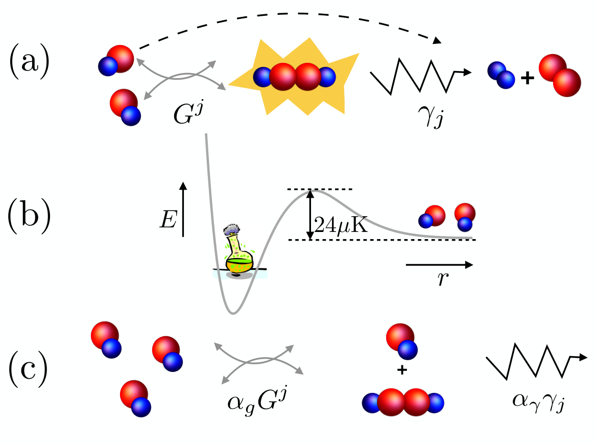
Figure 1: Schematics of the reactive collision processes.
(a) Two KRb molecules coherently collide in the -wave channel with rate to form an intermediate complex ,
which subsequently decays to the reaction products and at a rate . If the complex decay rate is the fastest process, as for KRb molecules, the complex can be adiabatically eliminated, giving rise to an effective two-body decay. (b) This recovers the standard picture of direct chemical reactions via p-wave inelastic collisions, where chemical reactions occur with unit probability at short-range inside the centrifugal barrier. (c) Additional (in)elastic complex-molecule collisions with rate effectively generate three-body molecule processes which can suppress the two-body molecule decay rate.
The use of spin-polarized fermionic molecules facilitated experimental efforts to reduce the undesirable chemical reactions as in these systems the collisions are dominated by -wave scattering. In this case, according to the Bethe-Wigner threshold law bethe1935theory; wigner1948behavior; sadeghpour2000collisions, chemical reactions are partially suppressed by the centrifugal barrier resulting in a loss rate that scales linearly with temperature . A quantitative analysis using a multichannel quantum defect theory (MQDT) greene1982general; idziaszek2010universal captured this behavior with a universal decay constant which well explained the experimentally observed decay rate in a gas of KRb molecules prepared in the classical regime (, with the Fermi temperature) de2019degenerate; ospelkaus2010quantum. However, the Bethe-Wigner threshold law has been shown to fail in a recent experiment de2019degenerate which prepared for the first time a quantum degenerate gas of KRb molecules in a D dipole trap reaching temperatures below .
Deep in the quantum degenerate limit (), a significant suppression of the loss rate compared to the one predicted by the MQDT theory was observed and conjectured to be a consequence of the underlying Fermi statistics.
Yet, this explanation is inconsistent with the naive expectation that, as the temperature vanishes, the Fermi pressure sets a lower bound for the -wave reaction rate, which would instead lead to a rate higher than the one predicted by purely classical arguments. The observed suppression therefore requires an explanation more profound than just Fermi statistics.
Recent experiments hu2019direct; liu2020steering moreover revealed that even in reactive molecules such as KRb, chemical reactions occur via the formation of a transient complex whose properties may affect the collision outcome. These observations therefore have opened the possibility of richer chemical reaction processescroft2020unified.
Here we provide a possible explanation of the observed chemical reaction suppression at ultracold temperatures by developing a theoretical many-body framework that accounts for the formation of molecular complexes. The large decay rate of the complex hu2019direct; liu2020steering allows us to adiabatically eliminate the complex, and obtain an effective two-body decay of the molecules which recovers the standard description of KRb chemical reactions. We analytically solve the rate equations, accounting for both heating effects and quantum Fermi statistics. We obtain a decay rate that is in agreement with the classical Bethe-Wigner threshold laws above quantum degeneracy, and also valid in the ultracold quantum regime. However, this model fails to capture the experimental observations in the quantum degenerate regime.
We therefore turn to an effective description, modelling beyond two-body physics by including effective elastic and inelastic complex-molecule interactions possibly emerging from many-body and effective medium effects at finite densities and in the presence of trapping light, which can generate a loss suppression mechanism alike to the one observed in the experiment.
The model.
We begin by deriving a framework including an intermediate complex, whose existence has recently been experimentally demonstrated hu2019direct; liu2020steering, formed via the collision of two molecules as illustrated in Fig. 1(a), which recovers standard chemical reaction rate equations.
We consider fermionic molecules, with mass confined by an external potential , which for simplicity we first set to be a simple square well that defines a confinement volume . In this system momentum is a good quantum number.
For molecules prepared in a single internal quantum state, -wave scattering dominates the collisions at ultracold temperatures due to Fermi statistics, which is, thus, the only partial wave we include.
Assuming there are multiple channels to form a complex (each denoted by j) the collision processes can be modeled by a simplified master equation
(1)
(2)
(3)
(4)
where is a fermionic creation(annihilation) operator of a molecule with momentum
, is a bosonic creation(annihilation) operator of a complex formed via channel , and the single-particle energies of the molecules and complexes respectively, with the binding energy of a complex. The parameter sets the complex-molecule collision strength and is the complex decay rate.
The Lindblad term,
, describes the action of an operator on the density matrix of the complex-molecule many-body system.
From the master equation one can obtain equations of motion of the relevant observables.
Since for the problem of interest the initial state has zero coherence terms and for , these terms can be neglected during the dynamics giving rise to the following equations:
(5)
(6)
(7)
with , and . The mean complex decay rate has been measured to be MHz in free space and even larger in the presence of trapping light liu2020steering. Because this rate is much larger than any other energy scales of the molecular gas de2019degenerate, we can adiabatically eliminate the complexes, and set to zero the left hand side of Eq. (6) and
. The complex-molecule coherence term then obeys:
supp.
Using this in Eqs. (5) and (7) recovers the standard equations that describe direct chemical reactions, if we identify the -wave collision parameters in terms of the real and imaginary parts of the scattering volume as follows: and (see supp). The real part describes elastic collisions that thermalize the system, and the imaginary part gives rise to the reactive collision rate julienne2009ultracold as illustrated in Fig. 1(b). We observe that in the limit of a large decay rate , we are in the quantum Zeno regime Misra1977; Itano1990; Zhu2013 where the decay of the molecules is limited by the formation of the complex, and in fact, is suppressed with increasing .
We find that the dynamics of the particle decay is mainly determined by the inelastic part since the elastic collisions conserve the total particle number and only slightly affect the decay rate by redistributing the mode population (see details in supp). Thus, in the following discussion, for simplicity we set . In this case the corresponding rate equations simplify to
(8)
with . The complex population adiabatically follows the molecule population as .
We can easily generalise Eq. (8) to any type of trapping potential by considering the corresponding single-particle eigenmodes.
Explicitly,
(9)
(10)
where denotes the molecule population operator
in mode , is given by an integral over eigenmodes and (see supp), and we defined the time-dependent averaged particle decay rates as
.
Comparison with Experiment
We now apply this developed framework to the experimental conditions, assuming a D harmonic trapping potential of the form
with the trapping frequency in the -th direction.
We also assume (m) for KRb molecules as calculated idziaszek2010universal and experimentally verified in the classical temperature limit de2019degenerate.
In addition to the total particle number , we study the density , the volume , defined as with the standard deviation of the density profile in the -th direction, the total energy and the energy density .
To develop an analytical understanding, we explore the scaling relations of the averaged decay rates and the volume.
For an equilibrium system at temperature ,
the population obeys the Fermi-Dirac distribution, from which the energy density , and
can be obtained as a function of .
As shown in Fig. 2 (a), in the classical limit ,
the energy density in each direction is in the harmonic trap in accordance with the equipartition theorem,
giving rise to ;
in the quantum degenerate limit , is higher than the one predicted by a classical scaling since the Fermi energy remains finite at zero temperature due to quantum statistics.
Figure 2:
Thermodynamic scaling relations in a D harmonic trap: (a) Average energy density, , (b) and (c) average volume, .
Numerical results are shown as blue dots, and analytical scalings as a function of energy density [red lines (bi,ci)] and temperature [black lines (bii,cii)]. Only the scaling in terms of remains valid in the quantum degenerate regime.
As demonstrated in Fig. 2 (b),
the scaling relations, and , written as a function of ,
are universal over the whole temperature range, whereas only in the classical regime the replacement is valid as shown in Fig. 2 (b.ii) and (c.ii).
During the non-equilibrium decay dynamics these simple relations derived in equilibrium are not necessarily applicable. Notwithstanding, they are found to keep holding during the full dynamics as benchmarked by numerical simulations (see supp). We attribute this partly to the fact that in a harmonic trap the initial Fermi distribution remains approximately unchanged during the dynamics by the balancing between the local density and the p-wave decay rate: the low energy modes with a low p-wave decay rate concentrate at the trap center where the density is higher, while the high energy modes with faster decay rates, concentrate at the edges where the density is lower, making the effective decay rate nearly uniform through the cloud.
In the experiment there is additional heating as particles are lost (see supp) similar to the one observed in prior experiments urvoy2019direct. Here we phenomenologically describe these heating processes by a background single particle heating rate acting as:
(11)
where and , and the subscript denotes the values at .
The dynamics of the density can be analytically obtained as
(12)
From this expression the density decay rate, which was the fitting parameter used to characterize the decay rate in Ref. de2019degenerate, is predicted to be at short times , and thus proportional to the energy density. In the classical limit, it recovers the results of the Bethe-Wigner threshold law since . In the quantum degenerate limit, the decay rate saturates to the Fermi energy instead of decreasing to zero.
Figure 3: Comparison of theory predictions considering pure p-wave molecule-molecule collisions without (red dots) or with (blue dots) additional complex-molecules collisions assuming , and experimental measurements (black dots). Each dot corresponds to different experimental runs with slightly different conditions (supp). The theory (experiment) is obtained as the best fit of the theoretically derived (the experimentally measured) to Eq. (12).
The error bars include uncertainties in the experimental measurements and the standard deviation from the fitting procedure (see details in supp).
In the classical temperature limit, both the theory and the experimental results are approximately constant, in agreement with the universal prediction idziaszek2010universal indicated by the gray band accounting for errors in the scattering value .
In the quantum degenerate limit, the model including the complex-molecule collisions can quantitatively reproduce the observed suppression.
To directly compare with the experimentally extracted rates, we numerically extract the decay rate as the best fit of to Eq. (12) for the corresponding initial conditions (see supp for detailed fitting procedures).
As shown in Fig. 3, the theory resuls are flat throughout both the classical temperature and the quantum degenerate regime, while the experimental data shows a strong suppression in the latter. We note that both represent an enhancement compared to the classical expectation where the decay rate would vanish in the zero temperature limit.
Beyond two-body molecule loss
Having established that pure two-body molecule decay is insufficient to explain the experimentally observed suppression, we consider more complicated interaction processes in our model. A change of the effective loss rate in our framework requires either the coherent coupling of molecules to complexes or the incoherent decay of the complexes themselves to be modified. Modifications to the former may arise from higher-order elastic interactions between molecules during complex formation, while modifications to the later could arise from inelastic complex-molecule decay channels due to for example light-assisted collisions. In fact, recent measurements of complex decay rates in KRb liu2020steering as well as other non-reactive molecules Cornish observed significant enhancement of the complex decay rate via photo-excitation processes.
In the following we explore such type of (in)elastic collisions between molecules and the complex, as illustrated in Fig. 1(c).
To connect to Eq. (4), for simplicity we start again by considering a homogeneous gas and model these processes by adding the following terms in the master equation
(13)
where the parameters and , which have the unit of , parametrizes the rates of three body elastic collisions and the molecule-complex decay respectively.
After adiabatically eliminating the complex, these terms result in a modification of the two-body decay rate and an additional molecular three-body decay term supp
(14)
where is the density of the molecular gas and we assumed .
Consequently, the total number of molecules follows
(15)
where the modified decay rate becomes , with an effective inelastic scattering parameter and .
Thus, counter-intuitively the additional loss due to complex-molecule collisions results in an effective suppression of the two-body loss due to the quantum Zeno effect which suppresses the population of the complex for larger loss rates.
For a gas trapped in a D harmonic potential this density dependent scattering strength generates an effective loss suppression in the quantum degenerate regime if as the gas becomes denser with decreasing temperature. In a system with a fixed particle number, where the change in density is directly correlated with the average volume, this suppression of the decay rate is tied to the temperature dependence of the average volume, see Fig. 2(c), reflecting the underlying Fermi statistics.
In Fig. 3 we demonstrate that this effective model can reproduce the experimentally observed suppression when choosing . However, we note that this corresponds to an inelastic collision rate between molecules and the complex which exceeds the unitary limit. In contrast, the elastic term is in principle feasible, but requires a coherent three body process, rather than the conventionally expected pure loss in a three-body collision Esry1999; Esry2001. A full explanation of the underlying many-body framework responsible for the emergence of this terms, either from quasi-particle dressing and in medium interactions, or direct multi-body or light assisted collisions is still pending.
Conclusions and outlook
We have developed a theoretical framework that accounts for the formation of an intermediate molecular complex to study the reactive dynamics of a quantum degenerate gas of polar molecules.
The first part of this work considering pure p-wave collision of the molecules establishes a decay rate proportional to the energy density of the gas, extending the classical Wigner threshold law to the quantum degenerate regime, and predicts a flat behaviour at low temperature enhanced compared to the linearly in T vanishing classical prediction.
However, as two-body molecule decay processes mediated by the formation of complexes alone does not reproduce the experimentally observed behaviour in the quantum degenerate regime, we considered beyond two-body molecule collisions. By including elastic or inelastic higher order complex-molecule interactions we are able to reproduce the experimental observations. Nevertheless, it seems unlikely that the actual origin of these terms are direct complex-molecule collisions. Instead they may emerge from many-body effects in the presence of trapping light. We hope that our conclusions can stimulate further theory work understanding the microscopic origin of these effects and experimental work that can directly validate or refute our predictions.
Acknowledgements.
We acknowledge helpful discussions with Jun Ye and his JILA KRb group, Joseph Thywissen, Paul Julienne, John Bohn and Qi Zhou during the preparation of this manuscript. This work is supported by the ARO single investigator award W911NF-19-1-0210, the DARPA DRINQs program and the JILA-PFC PHY-1734006 grants, by NIST, and by NSF grant PHY–1912350.
References
(1)
Luigi De Marco, Giacomo Valtolina, Kyle Matsuda, William G Tobias, Jacob P
Covey, and Jun Ye.
A degenerate fermi gas of polar molecules.
Science, 363(6429):853–856, 2019.
(2)
Lincoln D Carr, David DeMille, Roman V Krems, and Jun Ye.
Cold and ultracold molecules: science, technology and applications.
New Journal of Physics, 11(5):055049, 2009.
(3)
Steven A Moses, Jacob P Covey, Matthew T Miecnikowski, Deborah S Jin, and Jun
Ye.
New frontiers for quantum gases of polar molecules.
Nature Physics, 13(1):13, 2017.
(4)
Steven A Moses, Jacob P Covey, Matthew T Miecnikowski, Bo Yan, Bryce Gadway,
Jun Ye, and Deborah S Jin.
Creation of a low-entropy quantum gas of polar molecules in an
optical lattice.
Science, 350(6261):659–662, 2015.
(5)
Loïc Anderegg, Benjamin L Augenbraun, Yicheng Bao, Sean Burchesky,
Lawrence W Cheuk, Wolfgang Ketterle, and John M Doyle.
Laser cooling of optically trapped molecules.
Nature Physics, page 1, 2018.
(6)
S Ospelkaus, K-K Ni, D Wang, MHG De Miranda, B Neyenhuis, G Quéméner,
PS Julienne, JL Bohn, DS Jin, and J Ye.
Quantum-state controlled chemical reactions of ultracold
potassium-rubidium molecules.
Science, 327(5967):853–857, 2010.
(7)
Hans Albrecht Bethe.
Theory of disintegration of nuclei by neutrons.
Physical Review, 47(10):747, 1935.
(8)
Eugene P Wigner.
On the behavior of cross sections near thresholds.
Physical Review, 73(9):1002, 1948.
(9)
HR Sadeghpour, JL Bohn, MJ Cavagnero, BD Esry, II Fabrikant, JH Macek, and ARP
Rau.
Collisions near threshold in atomic and molecular physics.
Journal of Physics B: Atomic, Molecular and Optical Physics,
33(5):R93, 2000.
(10)
Chris H Greene, ARP Rau, and U Fano.
General form of the quantum-defect theory. ii.
Physical Review A, 26(5):2441, 1982.
(11)
Zbigniew Idziaszek and Paul S Julienne.
Universal rate constants for reactive collisions of ultracold
molecules.
Physical review letters, 104(11):113202, 2010.
(12)
M-G Hu, Y Liu, DD Grimes, Y-W Lin, AH Gheorghe, R Vexiau, N Bouloufa-Maafa,
O Dulieu, T Rosenband, and K-K Ni.
Direct observation of bimolecular reactions of ultracold krb
molecules.
Science, 366(6469):1111–1115, 2019.
(13)
Yu Liu, Ming-Guang Hu, Matthew A Nichols, David D Grimes, Tijs Karman, Hua Guo,
and Kang-Kuen Ni.
Steering ultracold reactions through long-lived transient
intermediates.
arXiv preprint arXiv:2002.05140, 2020.
(14)
James FE Croft, John L Bohn, and Goulven Quéméner.
A unified model of ultracold molecular collisions.
arXiv preprint arXiv:2005.13148, 2020.
(15)
****.
Supplementary information.
***.
(16)
Paul S Julienne.
Ultracold molecules from ultracold atoms: a case study with the krb
molecule.
Faraday discussions, 142:361–388, 2009.
(17)
B. Misra and E. C. G. Sudarshan.
The zeno?s paradox in quantum theory.
Journal of Mathematical Physics, 18(4):756?763, 1977.
(18)
Wayne M. Itano, D. J. Heinzen, J. J. Bollinger, and D. J. Wineland.
Quantum zeno effect.
Phys. Rev. A, 41:2295–2300, Mar 1990.
(19)
B. Zhu, B. Gadway, M. Foss-Feig, J. Schachenmayer, M. L. Wall, K. R. A.
Hazzard, B. Yan, S. A. Moses, J. P. Covey, D. S. Jin, J. Ye, M. Holland, and
A. M. Rey.
Suppressing the loss of ultracold molecules via the continuous
quantum zeno effect.
Phys. Rev. Lett., 112:070404, Feb 2014.
(20)
Alban Urvoy, Zachary Vendeiro, Joshua Ramette, Albert Adiyatullin, and Vladan
Vuletić.
Direct laser cooling to bose-einstein condensation in a dipole trap.
arXiv preprint arXiv:1902.10361, 2019.
(21)
Philip D Gregory, Jacob A Blackmore, Sarah L Bromley, and Simon L Cornish.
Loss of ultracold rb 87 cs 133 molecules via optical excitation of
long-lived two-body collision complexes.
Physical Review Letters, 124(16):163402, 2020.
(22)
B. D. Esry, Chris H. Greene, and James P. Burke.
Recombination of three atoms in the ultracold limit.
Phys. Rev. Lett., 83:1751–1754, Aug 1999.
(23)
B. D. Esry, Chris H. Greene, and H. Suno.
Threshold laws for three-body recombination.
Phys. Rev. A, 65:010705, Dec 2001.
(24)
M Holland, J Williams, and J Cooper.
Bose-einstein condensation: Kinetic evolution obtained from simulated
trajectories.
Physical Review A, 55(5):3670, 1997.
(25)
K-K Ni, S Ospelkaus, D Wang, G Quéméner, B Neyenhuis, MHG De Miranda,
JL Bohn, J Ye, and DS Jin.
Dipolar collisions of polar molecules in the quantum regime.
Nature, 464(7293):1324, 2010.
I Derivations of the rate equations
Here we first derive the equations of motions described by Eq. (1-4) in the main text.
We define and
)
(16)
(17)
(18)
(20)
Assuming the observables can be factorized as
(21)
(22)
then the equations of motion above become a closed set of equations and the dynamics of the observables can be evaluated. Our numerical simulations confirm the coherence terms , () and (), which are initially zero, remain zero, and therefore can be neglected. Then the relevant observables are ,
and .
In Ref. liu2020steering, the lifetime of the KRb complex was measured to be ns,
indicating MHz.
Since the experimentally relevant energy scales are set by the Fermi energy ( kHz), which is much smaller than the complex decay rate, we can adiabatically eliminate the complex, and set to zero both the left hand side of Eq. (18) and the term
.
Then the correlation terms can be approximated as
(23)
where and the second approximation is taken since the coherence term is zero. There we have also ignored single particle kinetic energy terms since they are in the order of .
By substituting the correlations into Eq. (), the dynamics for the molecular population becomes
(24)
Note that Eq. (24) recovers the standard rate equations that describe direct chemical reactions, if we identify and , with and the real and imaginary parts of the scattering volume.
As mentioned in the main text, Eq. (24) can be generalized to account for any type of trapping potentials by replacing by the population as given by
(25)
where with
(26)
where is the eigenfunction of the eigenmode of the single particle Hamiltonian.
II Effects of the elastic scattering
As discussed in the last section, both elastic and inelastic interactions are present.
According to the multichannel quantum defect theory (MQDT) idziaszek2010universal,
the elastic and inelastic scattering volumes in KRb have exactly the same amplitude but with opposite sign.
However, thermalization effect of the elastic collision cannot be captured by a second order cumulant expansion such as the one used to derive Eq. ()
Instead here we use kinetic theory to incorporate thermalization processes induced by elastic collisions holland1997bose and demonstrate that for the case of KRb they play a minimal role in the loss dynamics. In the context of kinetic theory the rate equations read:
where and is the single particle energy of mode .
Note that even though the elastic collisions are responsible for thermalization, the loss dynamics
is mainly determined by the inelastic part since the elastic collisions conserve the total particle number and only slightly affect the decay rate by redistributing the mode population, as shown in Fig. 4.
Figure 4: Population dynamics for different elastic scattering volumes and temperatures: (a) , (b) .
Panel (i) and panel (ii) show the particle mode distribution for particles () for and respectively.
The different colors represent the distribution at different times : blue: , yellow: ,
green: , red: and purple: .
Panel (iii) plot the dynamics of the particle number as a function of time (red: , blue dashed: ).The comparison shows that the elastic collisions only slightly affect the decay rate by redistributing the density profile and do not affect the decay dynamics.
To account for the fact that our simulations can not be done for large systems, we capture the effect of the elastic interactions expected for the real particle number used in the experiment , by rescaling both and by a factor of , given
the known scaling of .
III Evaporative heating
During the decay process, the evolution of the total energy of the system is given by:
(28)
where the time-dependent averaged particle decay rate is defined as
.
This equation together with the dynamics of , can be used to solve for
the dynamics of the energy density which evolves as
(29)
where
denotes the evaporative cooling(heating) rate with negative(positive) value.
For the D harmonic confinement under consideration,
the particles with lower energy decay faster according to the scaling . Therefore
the energy density increases as particles get lost and the system is evaporatively heated up.
Using the numerical results in Fig. 5,
is found to be a constant for all regimes down to
which is close to the result in the classical regime predicted in ni2010dipolar using a kinetic theory formalism.
Figure 5: The scaling relation is valid over a wide range of that covers both the classical limit and the quantum degenerate regime.
IV Simplified analytical equations
The experiment measured the decay dynamics of an ensemble of particles, for which a quantitative theoretical comparison is numerically hard, even at the mean-field level.
To overcome this numerical complexity as well as getting more insight into the decay,
we assume that the decay dynamics is governed by simple analytical equations which are valid when the system is in equilibrium.
Surprisingly, by performing comparisons with numerical calculations we find that these relations describe well the decay dynamics as shown in Fig. 6
Figure 6: Comparisons between the analytical results (red curves) and the numerical results (blue dashed lines) for the population dynamics at different initial equilibrium temperatures , and from bottom to top for particles.
We find that the analytical results can well capture the numerically obtained dynamics over a wide range of temperatures.
V Incorporating complex-molecule collisions in the rate equations
Taking into account the complex-molecule collisions, the equations of motions for the relevant observables become
(30)
where is the complex population operator.
Here we have neglected the kinetic energy term and the binding energy term. In addition, since the complex decay rate is large, it’s fair to assume that the complex population can be neglected when it is compared to the molecule population.
Therefore, by addiabatically eliminating the complex, one can obtain
(33)
(34)
where is the density of the molecules.
Similarly, by substituting the correlations into Eq. (30), the dynamics for the molecular population becomes
(35)
Here we have assumed approximation that is found to be valid for the KRb experimental parameters. In addition, we assume since the only the close to resonance complex can be formed.
And the dynamical equation for the total number of the molecules is given by
(36)
By comparing Eq. (35) with Eq. (24), we find the modified decay rate after taking into account of the inelastic molecule-complex collisions becomes
(37)
indicating that the effective inelastic scattering parameter becomes
(38)
VI Revised decay rates
In a harmonic trap, the density of the gas is not homogeneous, therefore the spatial dependence of the effective scattering coefficient needs to be taken into account.
This leads to a revised decay rate given by
(39)
Consequently, the revised rate equations for the mode populations are given by
(40)
where
The scaling of for systems with a large number of particles is limited by the computation complexity.
To overcome this limit, here we instead take the local density approximation starting from a semi-classical phase space distribution given by
(41)
the averaged decay rate can be calculated as
(42)
where and denotes the particle number and the volume respectively,
and the first term in the integrand accommodates the spatial dependence,
the second term represents the -wave collisional kernel that is proportional to the kinetic energy of the gas,
and the denominator is simply the total particle number of the system.
We compute the integral Eq. (42) numerically assuming different and particle number .
As shown in Fig. 7, we find that the ratio assuming )
saturates at high temperature and gets suppressed as the gas enters quantum degeneracy ( is calculated using Eq. (42).
In addition, the degree of suppression and the saturation temperature increase with increasing particle number.
Figure 7: The plots show for different (a) values assuming and (b) different particle number setting .
VII Fitting Analysis
In the experiment, the molecules are created and cooled down to the Fermi degenerate regime.
By fitting the initial density profile to a Fermi-Dirac distribution, the initial temperatures and are obtained.
To keep track of the reactive collision processes,
the particle number and the volume are measured as a function of the evolution time .
To compare with the experimentally extracted decay rate, both
the experimental initial energy density and the initial particle number are needed as an input parameters for the theory. They are extracted by a fitting procedure:
By fitting to ,
the initial energy density
and the linear heating rate can be extracted
with and the uncertainties.
Furthermore, by finding the best fit of to the theoretical obtained, the initial particle number can be obtained.
Assuming and ,
together with the extracted parameters , can be solved self-consistently.
The theoretically predicted is extracted from a linear fit to .
The comparison of the theoretically predicted and the experimentally measured are shown in Fig. 8.
We find that for the fixed used in the theory model, the theory results roughly agree with the experimental ones in the degenerate regime where the density is high,
while the theory overestimates the heating rates in the classical regime where the density is low, which is qualitatively consistent with the conjecture that the background heating is induced by the density-dependent collisions and should be smaller for dilute systems.
Figure 8: Comparison between the theoretically predicted (red dots) and the experimental measured (black dots) heating rates.
The theory predicted is obtained by substituting theoretically calculated decay rate , the heating rate , and the experimentally measured initial conditions and
into Eq. (12).
In Fig. 9, we compare the dynamics of predicted by the theoretical results and the experimental data.
The decay rate is obtained as the best fit of the theoretical to Eq. (12).
To incorporate the effect of the formation of the complex, we replace by . Since gives rise to suppression,
the agreement between the dynamics of the particle number of the theoretical results and experimental data becomes better, as shown in Fig. 9.
Figure 9:
Comparison between theoretical results and experimental data (black dots) for the particle number .
The theoretical results are obtained using the decay rates (red bands) and the revised decay rates (blue bands) respectively, where the ratio is calculated assuming .