Disentangling supercohomology symmetry-protected topological phases in three spatial dimensions
Abstract
We build exactly solvable lattice Hamiltonians for fermionic symmetry-protected topological (SPT) phases in ()D classified by group supercohomology. A central benefit of our construction is that it produces an explicit finite-depth quantum circuit (FDQC) that prepares the ground state from an unentangled symmetric state. The FDQC allows us to clearly demonstrate the characteristic properties of supercohomology phases - namely, symmetry fractionalization on fermion parity flux loops – predicted by continuum formulations. By composing the corresponding FDQCs, we also recover the stacking relations of supercohomology phases. Furthermore, we derive topologically ordered gapped boundaries for the supercohomology models by extending the protecting symmetries, analogous to the construction of topologically ordered boundaries for bosonic SPT phases. Our approach relies heavily on dualities that relate certain bosonic -group SPT phases with supercohomology SPT phases. We develop physical motivation for the dualities in terms of explicit lattice prescriptions for gauging a -form symmetry and for condensing emergent fermions. We also comment on generalizations to supercohomology phases in higher dimensions and to fermionic SPT phases outside of the supercohomology framework.
I Introduction
Symmetry-protected topological (SPT) phases of matter are classified by quantized invariants that capture a characteristic response to probing with symmetry defects [1, 2, 3, 4, 5, 6, 7, 8, 9, 10, 11, 12, 13, 14]. SPT phases built from fermionic degrees of freedom (d.o.f.) must conserve fermion parity, and the associated fermion parity symmetry defects can be used to probe the system. Consequently, the classification of fermionic SPT (fSPT) phases, where the constituent d.o.f. may be fermions, is notably distinct from the classification of bosonic SPT (bSPT) phases, composed of only bosonic d.o.f.. In particular, in three spatial dimensions and with unitary internal symmetries, the bSPT phases are believed to be classified by group cohomology, while the fSPT phases are only partially classified by the more rich, group supercohomology theory [12, 15, 16, 6, 17].
The algebraic data of group cohomology can be used to construct an exactly solvable model belonging to a bSPT phase [15]. The celebrated group cohomology models yield a transparent connection between the quantized invariant - namely, a group cocycle - and a lattice Hamiltonian. Another feature of these models is that a finite-depth quantum circuit (FDQC) [18] that prepares the ground state from a tensor product state can be written expressly in terms of . Further, in Ref. [19], it was shown that the group cohomology data could be used to identify symmetric topologically ordered gapped boundaries for the group cohomology models, by enlarging the protecting symmetry group on the boundary.
In this work, we construct exactly solvable models for ()D fSPT phases directly from the group supercohomology data that characterizes the phases. The resulting supercohomology models describe fSPT phases protected by finite unitary internal symmetries of the form , where denotes the fermion parity symmetry. The supercohomology data can be written as a certain pair of -dependent functions , where heuristically, corresponds to the data that characterizes the bSPT phases, while captures a response that is intrinsic to fSPT phases [13, 14]. With this, our principal contributions can be stated as follows. For any choice of supercohomology data characterizing a D fSPT phase:
- (i)
We construct a representative fSPT Hamiltonian with mutually commuting un-frustrated terms and verify that the quantized responses of the model correspond to the data - by explicitly computing the -symmetry fractionalization on fermion parity fluxes.
- (ii)
We identify a FDQC that prepares the ground state from a symmetric product state and determine the stacking rules for supercohomology phases from the composition of the FDQCs.
- (iii)
We use an extension of the symmetry to build symmetric topologically ordered gapped boundaries for the supercohomology model.
Our strategy is largely motivated by the spacetime formulation in Ref. [20], wherein fSPT phases are related to particular 2-group bSPT phases through a process of bosonization. More specifically, our construction can be broken down into the three succinct steps outlined below, and shown schematically in Fig. 1.

- (1)
Starting with a choice of supercohomology data , we first build an auxiliary bSPT model with a -group symmetry. The -group symmetry contains a -form symmetry as a subgroup.
- (2)
We gauge the -form subgroup by minimally coupling the model to a -form gauge field. This produces a symmetry-enriched gauge theory with an emergent fermion, referred to as the ‘shadow model’ [21].
- (3)
Finally, we pair the emergent fermion with a physical fermion and condense the composite excitation: the gauge theory is dual to a fermionic theory [22]. The result is a model for a fSPT phase characterized by the supercohomology data .
Relation to previous work:
Our work can be viewed as a generalization of the exactly solvable supercohomology models in D, described in Refs. [23, 24, 21]. Similarly, the first step is to construct an auxiliary bSPT model from the supercohomology data. In the case discussed here, however, the auxiliary bSPT phase is protected by a higher-form symmetry.
In the pioneering work of Ref. [16], representative wave functions for supercohomology phases were identified by studying re-triangulation invariant non-linear models on a discrete spacetime manifold. Later, Ref. [17] provided a comprehensive classification of fSPT phases on a spatial lattice, by solving for consistent domain wall decorations. Our work builds on these results by constructing an explicit parent Hamiltonian for their fixed point wave functions along with FDQCs that prepare the ground states from a product state. Within our framework, we are also able to demonstrate that the supercohomology models indeed exhibit the universal responses to symmetry fluxes captured by the supercohomology data .
Our strategy for constructing the supercohomology models mirrors the methods employed at the level of spacetime partition functions in Refs. [20, 25, 26]. In particular, Ref. [25] studies supercohomology phases by constructing a Lagrangian for the associated shadow model. However, we go beyond studying the shadow model and explicitly implement the fermionization duality to establish supercohomology data as quantized invariants of lattice Hamiltonians. In recent work, Ref. [26] constructed gapped boundaries for spacetime models of supercohomology phases using a symmetry extension (see also Ref. [27]). We employ a similar symmetry extension to construct the supercohomology Hamiltonians on a manifold with boundary.
We note that many of the models constructed in this text describe intrinsically interacting fSPT phases [8, 7]. That is, there are neither interacting bosonic counterparts nor free-fermionic representations of the phases. Hence, in particular, our work falls outside of the scope of Refs. [28, 29, 30].
Structure of the paper:
In Section II, we define the quantized invariants of supercohomology phases and present our supercohomology models in terms of the associated data. Subsequently, we describe the derivation of the bulk supercohomology models in Sections III and IV. In Section III, we give an example of our construction, for the case where the protecting symmetry is simply . We use the opportunity to introduce the notation of cohomology on a manifold , which is used throughout the text. Furthermore, in Section III.2 and Section III.3, we detail a lattice prescription for gauging a -form symmetry and condensing an emergent fermion, respectively. Section IV describes the construction of the supercohomology models more generally, where the protecting symmetry is . We show that the lattice Hamiltonians are indeed characterized by the supercohomology data and recover the additive group structure of supercohomology phases under the operation of stacking by composing the corresponding FDQCs in Section IV.4. Section V presents the symmetry extension method for constructing symmetric gapped boundaries for the supercohomology models; we leave the detailed derivation to Appendix L. In Appendix A, we compile the notation used in the text. We discuss spin structure and the bosonization duality of Ref. [22] in Appendix F. In Appendices J and K, we give a concise review the construction of supercohomology models in D and -group gauge theory, respectively. Lastly, Appendix M gives an example of the symmetry extensions used to construct the models with a boundary. The remaining appendices provide the technical details and explicit calculations used in the derivation of our models.
II Supercohomology models
Before discussing the construction of the supercohomology models in Sections III and IV, we give a concise description of the models themselves. We begin with a definition for the supercohomology data , and we assume familiarity with group cohomology. The group cohomology notation used here is summarized in Appendix A.1. In Section II.2, we then review the group cohomology models of Ref. [15]. We finish with Section II.3, where we define the more general supercohomology models and describe the stacking rules for the supercohomology phases, derived from the composition of FDQCs.
II.1 Supercohomology data
The supercohomology data gives quantized invariants for ()D fSPT phases protected by a finite onsite11 1 An onsite representation of a -form symmetry is a representation of in which, for all the representation is a tensor product of linear representations of on each site. unitary symmetry. To streamline the discussion, we refer to Appendix A.1 for a review of the notation from group cohomology. We freely use the notion of group cochains, the coboundary operator , and the cup- products with in the discussion below.
For a finite group , the supercohomology data is given by a pair of group cochains belonging to:
| (1) |
Furthermore, and satisfy the relations [16]:
| (2) |
Note that if , then is a group cocycle (). In this case, the supercohomology data reduces to the data that characterizes bSPT phases within the group cohomology framework [15].
The supercohomology data is further organized into equivalence classes. Two sets of supercohomology data and are considered equivalent if there exists:
| (3) |
such that:
| (4) |
In Section IV.4, we give physical motivation for the equivalence relation and show that if and are equivalent, then the corresponding supercohomology models belong to the same fSPT phase.
Throughout the text, we use the convention that group cochains are homogeneous. Therefore, in what follows, we take and to be functions:
| (5) |
which are homogeneous, i.e., for any :
| (6) |
II.2 Review of group cohomology models
When is zero, the supercohomology data is equivalent to the familiar group cohomology data, which characterizes ()D bSPT phases with a finite onsite unitary symmetry. As a consequence, the corresponding group cohomology models are a special case of the supercohomology models. We build up to the supercohomology models in Section II.3 by first reviewing the group cohomology models of Ref. [15].

The group cohomology models are defined on an arbitrary triangulation of an orientable closed -manifold . The triangulation of gives a decomposition of into vertices, edges, faces, and tetrahedra. We further require that the triangulation is equipped with a branching structure – an assignment of an orientation to each edge in such a way that there are no cycles around any of the faces. A branching structure yields both an ordering of the vertices of each tetrahedron as well as an orientation of any tetrahedron relative to the orientation of (see Fig. 2).
The Hilbert spaces for the group cohomology models are formed by placing a d.o.f. on each vertex of (Fig. 3). A basis for the dimensional Hilbert space at vertex is given by states labeled by elements of . Furthermore, a basis for the full Hilbert space is given by product states of the form , in which, the state at vertex is . The symmetry is represented using the regular representation, i.e., for any , is represented by:
| (7) |
The group cohomology models can be built from a -paramagnet Hamiltonian – a Hamiltonian belonging to the trivial SPT phase. The -paramagnet Hamiltonian is given by:
| (8) |
where the sum is over vertices in , and is a projector onto a symmetric state at the vertex , i.e.:
| (9) |
The ground state of the -paramagnet Hamiltonian is a tensor product of a symmetric state at each vertex. This can be written as an equal amplitude superposition over all configurations:
| (10) |
Here, as elsewhere in the text, we omit the normalization of the state for notational convenience.

We build the group cohomology model corresponding to the group cocycle by conjugating by a FDQC . is defined in terms of the data as [15]:
| (11) |
where the product is over all tetrahedra in , the vertices specifying the tetrahedron are ordered according to the branching structure, and , in the argument of , denotes the identity in . To simplify the notation, we introduce an operator , for each tetrahedron in :
| (12) |
With this, can be written more compactly as:
| (13) |
The Hamiltonian for the group cohomology model is then:
| (14) |
with the unique ground state:
| (15) |
The Hamiltonian indeed describes a bSPT phase. This is because the Hamiltonian is both symmetric and has a unique short-range entangled (SRE) ground state. The symmetry of the Hamiltonian follows from the fact that is symmetric, which can be shown using the property . The ground state is SRE, since it can be prepared from a product state by the FDQC .22 2 We note that, although is symmetric, this does not imply that the state in Eq. (15) belongs to the trivial SPT phase. This is only the case if can additionally be expressed as a FDQC composed of symmetric local unitaries. Furthermore, the group cohomology models exhibit the characteristic responses encoded by , as can be checked by introducing symmetry defects or gauging the symmetry and analyzing the properties of the symmetry fluxes [12, 9].
II.3 Definition of supercohomology models
We now generalize the discussion to supercohomology models, which describe fSPT phases. We leave the explicit derivation of the models from a choice of supercohomology data to Sections III and IV. Similarly to the group cohomology models, the supercohomology models are prepared from a Hamiltonian in a trivial SPT phase by conjugation with a FDQC. Further, the FDQCs for and can be used to recover the stacking laws for supercohomology phases, discussed at the end of this section.


The supercohomology models are defined on a Hilbert space with d.o.f. at the vertices of , as in the previous section, along with a fermionic d.o.f. at each tetrahedron.33 3 We note that the manifold admits a spin structure. This is always true for orientable -manifolds. Specifically, we place a single spinless complex fermion at the center of each tetrahedron and label the two Majorana operators at the tetrahedron by and (see Fig. 4). The fermion parity at is then given by:
| (16) |
and we also introduce a “hopping” operator that changes the fermion parity on either side of the face :
| (17) |
Here, and are the tetrahedra neighboring such that the orientation of points out of the tetrahedron and into the tetrahedron (see Fig. 5). corresponds to a choice of spin-structure and is determined by the branching structure of the triangulation of . We refer to Appendix F and Ref. [31] for the explicit form of . As before, the symmetry is represented with the regular representation, and here the global fermion parity symmetry is generated by .
The supercohomology models are built from a Hamiltonian belonging to a trivial fSPT phase - namely, an atomic insulator with a decoupled -paramagnet. The trivial fSPT Hamiltonian is explicitly:
| (18) |
The ground state of is a product state with zero fermion occupancy at each tetrahedron and a symmetric state at each vertex.
Given a choice of supercohomology data , we prepare the supercohomology model from by conjugation with the FDQC :
| (19) |
Let us unpack the notation used in the definition of . First of all, the term is analogous to the FDQC in Section II.2, tensored with the identity on the fermionic d.o.f.. Second, the product over hopping operators in Eq. (19) depends on a choice of ordering for the faces , since not all hopping operators commute. However, is an order dependent sign that compensates for the choice of ordering. Therefore, in the end, the FDQC is independent of the choice of ordering for the faces in . We give the explicit form of in Section IV.4.44 4 We note that while depends on a global ordering of the faces in , it can nonetheless be implemented by a FDQC. This can be seen from the derivation of in Appendix H.2. is the -dependent operator:
| (20) |
for an arbitrary face and implicitly tensored with the identity on the fermionic d.o.f.. Finally, for a tetrahedron , is shorthand for:
| (21) |
The exactly-solvable fermionic Hamiltonian produced by conjugating by is thus:
| (22) |
which has the unique ground state :
| (23) |
describes a system in a fermionic SPT phase, because (i) is symmetric and (ii) it has a unique, SRE ground state [Eq. (23)]. The Hamiltonian in Eq. (22) is symmetric, since both and are invariant under the symmetry – we argue that is symmetric in Section IV.4.55 5 Although is symmetric, it cannot be decomposed into a FDQC comprised of symmetric local unitaries. The ground state is unique and SRE, because is unitarily equivalent to a trivial fSPT Hamiltonian with a unique ground state and the unitary is a FDQC.
Most importantly, belongs to the fSPT phase characterized by the corresponding supercohomology data . We show this in Section IV.4, by gauging the fermion parity symmetry of . This results in a -symmetry-enriched gauge theory, where the symmetry fractionalizes on the fermion parity flux loops, as determined by . The appropriate responses to -symmetry defects follow from the bosonic, group cohomology case.
We can gain intuition for the fSPT Hamiltonian by inserting the right hand side of Eq (18) into the expression for :
| (24) |
By commuting the hopping operators of past the parity operator and using that , the tetrahedron terms become:
| (25) |
In the ground state, the fermion occupancy depends on the -configuration. For a -configuration , it is energetically preferable for the fermion occupancy at the tetrahedron to be equal to . In this way, complex fermions are bound to junctions of symmetry domains. The vertex terms of , on the other hand:
| (26) |
are more difficult to compute, in general. Heuristically, they fluctuate the d.o.f. and create, move, and annihilate fermions without affecting the tetrahedron terms in Eq. (25). The ground state is thus a weighted superposition of -configurations with the fermion occupancy at each tetrahedron equal to . This is in agreement with the fixed point wave functions in Ref. [17].

Stacking rules for supercohomology phases:
Having defined the models, we can now deduce the stacking rules for supercohomology phases. We recall that two states can be stacked by taking the tensor product. Given two -SPT states and , the stacked state also belongs to a -SPT phase. Thus, the stacking of -SPT states induces an operation at the level of the SPT phases.
In Ref. [23], it was argued that the stacking operation on SPT phases can be determined from the composition of FDQCs. To state the result from Ref. [23], we define and to be symmetric FDQCs that prepare the -SPT states and , respectively, from a symmetric product state. According to Ref. [23], if and belong to the same Hilbert space, then the composition of the FDQCs and prepares a state belonging to the same -SPT phase as .
With this, we determine the group law under stacking for D supercohomology phases by composing the FDQCs defined in Eq. (19). Given two sets of supercohomology data and both characterizing fSPT phases with a symmetry, we consider stacking the ground states of the corresponding supercohomology models, denoted by and , respectively. The result from Ref. [23] tells us that the stacked state belongs to the same phase as the state prepared by applying to a symmetric product state. Here, and are the FDQCs from Eq. (19) that prepare and from an unentangled symmetric state, respectively. In Appendix H.3, we show that the composition is equivalent to a FDQC corresponding to a set of supercohomology data :
| (27) |
Therefore, at the level of the supercohomology data, the stacking operation is:
| (28) |
in agreement with Ref. [16].
III Bulk construction:
We begin by illustrating our construction of exactly-solvable models for fSPT phases in the simplest possible case – for fSPT phases protected by only fermion parity symmetry . While the resulting fSPT model is trivial (an atomic insulator), we nonetheless find this example instructive in demonstrating the general strategy. Moreover, we use this as an opportunity to introduce notation used throughout the paper.
To start, we describe a model for a certain bosonic SPT phase protected by a -form symmetry in (3+1)D. The special property of this bosonic SPT is that, upon gauging the -form symmetry, we obtain a gauge theory with an emergent fermion. We refer to this gauge theory as the twisted toric code. In the final step, we employ the fermionization duality of Ref. [32] to map the twisted toric code to a model with a fundamental fermion. The construction is shown schematically in Fig. 6, for the case of .
III.1 -form SPT and notation
SPT phases protected by higher form symmetries, including -form symmetries, were first introduced in Ref. [33]. Subsequently, fixed point Hamiltonians for -form SPT phases were described in detail in Refs. [34] and [35]. We note that the Hamiltonian discussed in this section agrees with the model in Ref. [35] and is closely related to the -form SPT model of Ref. [34].66 6 Specifically, our model is equivalent to the model in Ref. [34] on a four-colorable triangulation and upon restricting to the diagonal of the symmetry.

Our model for a nontrivial -form SPT phase can be defined on an arbitrary triangulation of an oriented closed -manifold equipped with a branching structure, as described in Section II.2. We define a Hilbert space on using the triangulation of the manifold – at each edge of the triangulation, we place a single degree of freedom. Correspondingly, a basis for the Hilbert space at edge is given by states with valued in . The Pauli Z and Pauli X operators at each act as:
| (29) |
where addition is taken modulo . A basis for the total Hilbert space consists of states labeled by configurations (Fig. 7). Here, the state denotes a product state with the d.o.f. at edge in the state .
The -form symmetry acts on closed codimension- submanifolds of the dual lattice. In particular, we represent the symmetry action on a closed surface of the dual lattice with the operator:
| (30) |
where the product is over edges intersected by the surface (see Fig. 8).

We construct our model for the nontrivial SPT phase starting with a Hamiltonian for a -form paramagnet. The Hamiltonian for the -form paramagnet is given by:
| (31) |
is certainly symmetric, as it commutes with for every surface of the dual lattice. Further, the unique ground state of is a product state with the eigenstate of at each edge . This state can be expressed in the configuration basis as:
| (32) |
with the sum over all configurations .
Now, our model for the nontrivial -form SPT phase is built from the -form paramagnet in Eq. (31) by conjugation with the FDQC:
| (33) |
Specifically, the Hamiltonian of the nontrivial -form SPT model is:
| (34) |
Indeed, describes a nontrivial -form SPT phase. In the next section, we show this by gauging the -form symmetry. The -form paramagnet is mapped to a gauge theory with an emergent boson - the usual D toric code, while is mapped to a gauge theory with an emergent fermion - a “twisted toric code”.
For now, we note that the model in Eq. (34) is symmetric and exactly solvable. In Appendix B, we show that is symmetric under the -form symmetry. Consequently, is also symmetric. Furthermore, the model is exactly solvable, since by construction, the terms in are mutually commuting and unfrustrated. The unique ground state is then expressly:
| (35) | ||||

To further motivate this model, we recount the spacetime construction of the -form SPT phase in Ref. [35]. We consider a partition function for the SPT phase on the cone of , denoted , which is the D spacetime formed by connecting a single spacetime vertex to each vertex of the closed manifold as shown in Fig. 9. This produces a manifold with a boundary equal to . We refer to the edges connected to the additional spacetime point as “time-like” edges and extend the branching structure so that the time-like edges have an orientation pointing away from the additional spacetime vertex. Then, the partition function for the -form SPT model is [35]:77 7 Using notation introduced later in the text, the expression: can be written as . is a nontrivial -form cocycle that has been pulled back to .
| (36) |
with the product over spacetime -simplices. The amplitude for a fixed configuration :
| (37) |
is topological in the sense that it is invariant under re-triangulations of the spacetime manifold. Through re-triangulations, it can be seen that the values of on the time-like edges do not affect the amplitude. Therefore, we may set their value to , for simplicity. As a result, the amplitude for a configuration on reduces to:
| (38) |
where the product is over tetrahedra on the boundary of . This gives the amplitude for a wave function on with the configuration , as in Eq. (35). We remark that this construction parallels the approach for building -form SPT Hamiltonians in Ref. [15].
cohomology on
At this point, we find it convenient to introduce the language of cohomology on . The cohomology notation allows for compact expressions and, in our opinion, more transparent calculations. Here, we only describe the necessary ingredients, and we leave a more thorough summary to Appendix A.2. In the process of introducing concepts from cohomology on , we re-express the -form SPT model using the corresponding notation. In particular, we aim to write in an explicit form.
To begin, we define a -cochain as a linear, -valued function of -simplices in . For example, we can consider the -cochain defined by:
| (39) |
In words, evaluates to on the edge and on all other edges. More general -cochains can be formed from linear combinations of -cochains of the form in Eq. (39). Specifically, for each configuration we can define a corresponding -cochain as:
| (40) |
Evaluating on an edge gives:
| (41) |
Given the correspondence between -cochains and configurations in Eq. (40), we can label a configuration state by the -cochain :
| (42) |
In this notation, a Pauli Z operator at edge acts on the state as:
| (43) |
and an operator acts as:
| (44) |
Moreover, the action of the -form symmetry operator on a configuration state is:
| (45) |
where we have defined the -cochain as:
| (46) |
Next, we introduce the coboundary operator , which is a linear map taking -cochains to -cochains. Specifically, it maps a -cochain to the -cochain for which:
| (47) |
where is any -simplex and denotes a formal sum of -simplices in the boundary of . Simply put, the -cochain is evaluated on a -simplex by evaluating on the boundary components of . The coboundary of , for example, is a -cochain satisfying:
| (48) | ||||
for a face .
If the coboundary of a -cochain is , we call the -cochain closed. The -cochain in Eq. (46) is closed, i.e.:
| (49) |
This is because is a closed surface of the dual lattice. As such, for any face , the boundary of contains an even number of edges intersected by .
Further, we define the cup product . The cup product maps a -cochain and a -cochain to a -cochain . Specifically, evaluated on a -simplex is:
| (50) |
is evaluated on the -simplex formed by the first vertices, while is evaluated on -simplex formed by the last vertices.
A suggestive example of the cup product comes from considering . evaluated on a tetrahedron gives:
| (51) | ||||
Referring to Eq. (33), we see that the FDQC can be written as:
| (52) |
with the sum over all -cochains.
To simplify the notation, we use the shorthand:
| (53) |
where is a -cochain, is a -dimensional manifold, and the sum is over -simplices in . Throughout the text, unless specified otherwise, it should be assumed that the integral is over the manifold . In particular, we can make the replacement:
| (54) |
With this, the circuit is:
| (55) |
and the ground state in Eq. (35) is:
| (56) |
Lastly, we introduce the cup- product . Although abstract, the cup- product allows for a convenient form of the Hamiltonian and is key to our analysis of the twisted toric code in the subsequent section. The cup- product takes a -cochain and a -cochain to a -cochain . Explicitly, evaluated on a -simplex is:
| (57) | ||||
A useful example, relevant to our expression for , is the cup- product of and . Here, is the -cochain that evaluates to on the face and for all other faces:
| (58) |
The -cochain evaluated on a tetrahedron is [using Eq. (57)]:
| (59) | ||||

Now, with the notation from cohomology on , we can express in Eq. (34) in a compact form. In Appendix B, we show that:
| (60) |
Above, we have used to denote the product of around the face :
| (61) |
While the product in Eq. (60) is over all faces in , the Hamiltonian is indeed local. This is because , if the face and edge do not both belong to the tetrahedron . Heuristically, is “dressed” with loops of Pauli Z operators around certain faces near [Fig. 10].
III.2 Twisted toric code
The twisted toric code is constructed from in Eq. (60) by gauging the -form symmetry. In this section, we provide a physical description of the gauging procedure following the steps outlined in Ref. [1]. In Appendix C, we discuss the subtleties of the procedure and describe the process at the level of states, as in Ref. [34]. After gauging the -form symmetry of , we show that the resulting twisted toric code admits localized excitations with fermionic statistics.
The prescription for gauging a -form symmetry in Ref. [1] naturally generalizes to gauging a -form symmetry. In particular, the -form symmetry is gauged according to the following steps.
- 1.
We introduce d.o.f. on faces corresponding to -form gauge fields. We denote the Pauli Z and Pauli X operators at the face by and , respectively.
- 2.
We impose a gauge constraint at each edge :
(62) where the product is over faces containing . This constraint can be interpreted as a -form Gauss law. We note that the operator defines a local action of the -form symmetry. That is, a product of over edges intersected by a closed surface in the dual lattice yields the -form symmetry operator .
- 3.
To make coupling to the gauge field in the subsequent step unambiguous, we energetically enforce a “no flux condition”. The point-like -form gauge flux can be detected by the operator , where is a product of operators around a tetrahedron :
(63) Therefore, the no flux condition is enforced by adding to the Hamiltonian the term:
(64) In addition, we conjugate each Hamiltonian term by a local projector onto the zero flux subspace in the vicinity of the term. That is, for a Hamiltonian term whose support88 8 The support of an operator is the set of sites on which the operator acts non-identically. is contained in the bounded region , we conjugate by a projector:
(65) where the product is over tetrahedra in .
- 4.
We then minimally couple the -form symmetric model to the gauge fields, so as to make the model invariant under the gauge constraint. In particular, is coupled to the gauge field as:
(66) - 5.
We fix a gauge by mapping gauge invariant states to representative states in which the eigenvalue of is at every edge 99 9 More precisely, we can form an over-complete basis for the gauge invariant Hilbert space by projecting configuration basis states to the gauge invariant subspace with the operator: (67) Each gauge invariant state in this (over-complete) basis is a superposition of configuration states and includes exactly one state for which the eigenvalue of is at every edge. By gauge fixing, we mean that the over-complete basis states are mapped to the “representative” state with the eigenvalue of equal to at each edge. The representative states form a basis for the gauge fixed Hilbert space.. This gauge fixed Hilbert space is equivalent to a Hilbert space with only the gauge field d.o.f. on the faces. The action of on gauge invariant states is replaced by after fixing the gauge, and in Eq. (66) becomes equivalent to in the gauge fixed Hilbert space. Therefore, the gauge invariant operators and are mapped according to:
(68)
| Model with | Model with dual |
| -form symmetry | -form symmetry |
| 1 | |
| 1 |
We remark that, operationally, the gauging procedure is equivalent to a certain operator duality. In particular, the duality maps the -form symmetric operators and according to:
| (69) |
We have summarized the corresponding operator duality in Table 1, and we refer to Appendix C for further details.
As a result of applying steps 1-5 above to our model for the nontrivial -form SPT phase, we obtain the twisted toric code. The twisted toric code is defined on a Hilbert space composed of d.o.f. attached to each face of the triangulation of (Fig. 11). Further, a basis for the Hilbert space is given by the product states , where the state at the face is (with ). In analogy to Eq. (42), a configuration state can be labeled by a -cochain :
| (70) |
With this notation, the Pauli Z and Pauli X operators acting on the face can be written as:
| (71) |


By gauging the -form symmetry of [Eq. (60)], we find the twisted toric code Hamiltonian:
| (72) |
where is:
| (73) |
An example of the term is shown in Fig 12. For simplicity, we have omitted the local projectors from step 3 of the gauging procedure. They do not affect the discussion in this section. The terms of are all mutually commuting, since the gauging procedure preserves the commutation relations. We show in Appendix D that a ground state of the model is:
| (74) |
Note that while the expression for has a sum over -cochains , there are no d.o.f. on the edges. Rather, by summing over -cochains , is a ground state of with trivial holonomy.
Excitations in the twisted toric code:
There are two types of excitations of the twisted toric code. The first, is a line-like -form gauge charge corresponding to violations of the edge terms . A small loop of gauge charge around the face is created by acting with the face operator . A larger loop of gauge charge can be created by acting with on all faces contained in a 2D membrane of the direct lattice:
| (75) |
We think of the gauge charge as lying along the boundary of , since the membrane operator anti-commutes with the edge terms for which is in the boundary of .
The second type of excitation of is a point-like -form gauge flux corresponding to a violation of a term. A pair of gauge fluxes can be created at neighboring tetrahedra by the short string operator:1010 10 To avoid confusion with the operator in Ref. [22], we use .
| (76) |
pictured in Fig. 13. anticommutes with the tetrahedron terms on either side of the face . Thus, we interpret the gauge fluxes as living at the centers of tetrahedra. The Pauli Z operators in Eq. (76) ensure that for any and any , commutes with . The short string operators satisfy the commutation relations [22]:
| (77) |
for any faces and .
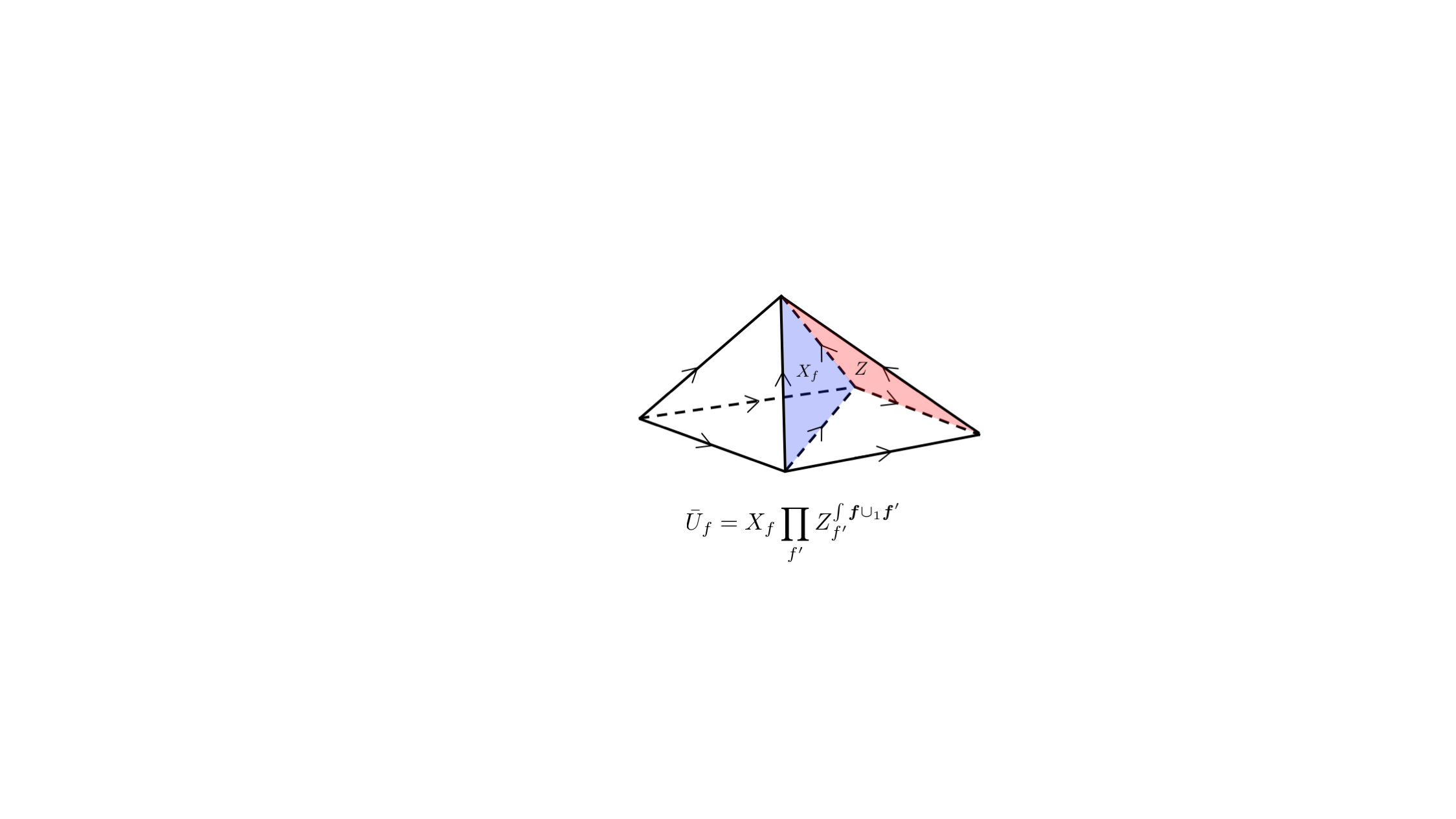
Longer string operators can be formed by composing the short string operators in Eq. (76). However, a simple product of operators along a path in the dual lattice is ambiguous. This is because, given the commutation relations in Eq. (77), a product of operators is generically order dependent. To remove the ambiguity, we define the following notation. For any set of faces, we define an order independent product of by:
| (78) |
Here, all of the Pauli Z operators from the definition of appear to the left of the Pauli X operators. We can then unambiguously define a gauge flux string operator along a path in the dual lattice by:
| (79) |
where denotes the set of faces intersected by .

Remarkably, the gauge fluxes are emergent fermions. To see this, we use the methods developed in Refs. [36] and [37] for computing the statistics of anyons from microscopic models. We consider three paths , , and along the dual lattice sharing a common endpoint, as in Fig. 14. The statistics of the gauge fluxes can be deduced by comparing the product to .
To gain intuition for this comparison, we imagine gauge fluxes at and in Fig. 14. In the first process , the gauge flux at is moved to and the gauge flux at is moved to . Whereas, in the second process , the gauge flux at is moved to and the gauge flux at is moved to . The final configurations of the gauge fluxes differ by an interchange of the position of the gauge fluxes. Consequently, the difference between and determines the statistics of the gauge fluxes.
It can be shown that the gauge flux string operator satisfies:
| (80) |
This follows from an explicit computation using the commutation relations of the operators in Eq. (77).1111 11 More precisely, this can be checked by explicitly computing the sign for each possible intersection at a tetrahedron. The sign for only four of the possible orientations of the tetrahedron needs to be verified, as the others follow from symmetries of the calculation. Therefore, the gauge fluxes are emergent fermions. We note that this is equivalent to saying that the twisted toric code has an anomalous -form symmetry [22, 20]. The -form symmetry, which, by definition, acts on closed codimension- subspaces, is generated by loops of the emergent fermion string operator. It is called anomalous, simply because the gauge fluxes have fermionic statistics.
Before leveraging our understanding of the twisted toric code to construct a model of physical fermions, we would like to point out that the emergent fermion string operator is not unique. In fact, we can define an alternative emergent fermion string operator built from the short segments:
| (81) |
with denoting the tetrahedron neighboring in the direction of the orientation of (see Fig. 5). The corresponding string operator along a path in the dual lattice is:
| (82) |
An important observation moving forward is that is equivalent to a small loop of string around the edge (see Appendix E):
| (83) |
where the path intersects only the faces adjoined at . Therefore, the operators are local generators of an anomalous -form symmetry. Since commutes with , we see explicitly that the twisted toric code has an anomalous -form symmetry.
III.3 Atomic insulator

The last step of our example is to convert the twisted toric code into a model with physical fermions. This can be accomplished by applying the D fermionization duality introduced in Ref. [22], reviewed in Appendix F. In this section, we instead opt to describe the fermionization process in terms of fermion condensation [38, 23]. That is, we construct the fermionic model by pairing emergent fermions with physical fermions and condensing the composite bosonic excitations. The fermion condensation procedure, described below, can be interpreted as a generalization of Refs. [1] and [39] to gauging an anomalous -form symmetry. Although an anomalous symmetry typically implies an obstruction to gauging the symmetry, we bypass the obstruction by employing fermionic d.o.f. for the gauge fields.
Our prescription for fermion condensation starts by introducing a spinless complex fermion d.o.f. at the center of each tetrahedron (Fig. 15). Thus, to prepare for the discussion of fermion condensation, we recall the notation for the operators on the fermionic Hilbert space, defined in Section II.3. The fermion parity operator at is:
| (84) |
and the hopping operator across the face is:
| (85) |
and are defined below Eq. (17), and is a formal sum of -simplices that amounts to a choice of spin-structure; see Appendix F for the explicit form of .1212 12 Note that every orientable -manifold admits a spin structure, so a choice of is guaranteed. The hopping operators satisfy the commutation relations:
| (86) |
which we note matches the commutation relations of in Eq. (77). Lastly, we define an alternative hopping operator , instrumental for the fermion condensation prescription below:
| (87) |

With notation for the fermionic d.o.f. defined, we can describe the fermion condensation procedure. Our procedure applies to any Hamiltonian with an emergent fermion created by the string operator in Eq. (82). In other words, the fermion condensation procedure applies to any Hamiltonian with an anomalous -form symmetry locally represented by the operators . Fermion condensation then proceeds as follows.
- 1.
We introduce a spinless complex fermion d.o.f. at each tetrahedron. In terms of gauging the -form symmetry, the anomalous nature requires that the “-form gauge fields” are fermionic d.o.f..
- 2.
We impose a gauge constraint:
(88) for each face . This constraint enforces a proliferation (or condensation) of composite excitations composed of an emergent fermion and a physical fermion. This is because is a short segment of emergent fermion string operator [Eq. (82)], which creates emergent fermions at the tetrahedra on either side of , while creates physical fermions at the corresponding tetrahedra (Fig. 16). Importantly, the constraints at different faces commute, due to the matching commutation relations of and (see Appendix E). We note that the gauge constraint in Eq. (88) is a local action of the anomalous -form symmetry, in the sense that the product of around an edge returns ; this is guaranteed by the spin structure dependent sign in the definition of the hopping operator.
- 3.
To make the Hamiltonian gauge invariant, i.e., commute with the constraints in Eq. (88), we couple the Hamiltonian to the fermionic d.o.f.. Since the Hamiltonian commutes with , it can be expressed in terms of and operators [22]. We couple operators and operators to the gauge fields as:
(89) To avoid possible ambiguity, we require that the coupling preserves the locality of the Hamiltonian. Any local, gauge invariant operators can be expressed in terms of the operators and .
- 4.
We fix a gauge in which the eigenvalue of is at each face . The action of on the constrained space is replaced by in the gauge fixed Hilbert space.1313 13 This can be seen by multiplying by . We obtain: acts as the identity in the fixed gauge. Further, the gauge invariant operator becomes after fixing the gauge. The generators of local, gauge invariant operators are thus mapped according to:
(90) The mapping in Eq. (90) produces a fermionic Hamiltonian defined on a Hilbert space with a single spinless complex fermion d.o.f. at each tetrahedron, as depicted in Fig. 15.
| Model with | Model with |
| emergent fermions | even fermion parity |
| 1 | |
| 1 |
By condensing the emergent fermion in the twisted toric code, we obtain a model for an atomic insulator. More specifically, applying the fermion condensation procedure to yields the atomic insulator Hamiltonian (Appendix E):
| (91) |
This Hamiltonian has a unique ground state , a product state with zero fermion occupancy at each tetrahedron. Excitations are physical fermions, where has eigenvalue .
The process of gauging a non-anomalous symmetry, such as the -form symmetry in Section III.2, can be stated as an operator duality [1]. Likewise, the fermion condensation procedure can be implemented by a mapping of operators. We summarize the corresponding duality in Table 2 and provide more details in Appendix F. Notably, the duality corresponding to fermion condensation maps:
| (92) |
Combining Eqs. (89) and (90), we see that the duality is functionally the same as the fermion condensation procedure outlined above.
IV Bulk construction:
We now generalize the discussion of Section III to construct fSPT models protected by a symmetry. In this case, we require a choice of supercohomology data . Therefore, before outlining the construction of the fSPT models, we first review the supercohomology data , and introduce corresponding cochains on the manifold . Then, we use the supercohomology data to build a -group SPT model, which, loosely speaking is protected by an interdependent -form and -form symmetry. Next, we gauge the -form symmetry of the -group to obtain the so-called shadow model – a symmetry-enriched twisted toric code. The shadow model is such that fermion condensation produces a model for the fSPT phase corresponding to the supercohomology data . The construction is shown schematically in Fig. 1.
IV.1 Supercohomology data on
In Section II.1, we introduced the supercohomology data as homogeneous functions:
| (93) |
which, as group cochains, satisfy the relations:
| (94) |
In what follows, we find it convenient to work with cochains on – functions of simplices in the triangulation of . Therefore, in this section, we describe how functions of variables, can be pulled back to cochains on .
We use the functions , , and as examples for describing the pull back of functions to cochains on . , , and are defined by:
| (95) | ||||
| (96) | ||||
| (97) |
with denoting the identity in . The pull backs of these functions play an important role in the construction of the supercohomology models below. We note that the functions are not group cochains, since they fail to be homogeneous.
To define cochains on , corresponding to , , and , we assign an element of to each vertex in the triangulation of . We refer to the set of labels as a -configuration. With labels on the vertices of , functions of can be pulled back to -cochains on . For each -configuration, we define the cochains , , and on satisfying:
| (98) | ||||
| (99) | ||||
| (100) |
for an arbitrary face , edge , and tetrahedron .
The Hamiltonians discussed below are defined on triangulated manifolds with a d.o.f. at every vertex, such as in Figs. 3 and 4, and a set of basis states can be labeled by -configurations. Hence, to simplify the notation in the construction of the supercohomology models, we introduce diagonal operators for each -dependent cochain on . The operator associated to the -dependent -cochain and a -simplex is defined as:
| (101) |
The operators associated to , , and are thus:
| (102) | ||||
| (103) | ||||
| (104) |
for a choice of face , edge , and tetrahedron . Unless otherwise stated, it should be assumed that the operators are tensored with the identity on any other d.o.f. in the model.
The coboundary operator and cup products can naturally be extended to the operators at the cochain level. For example, the coboundary of is the operator:1414 14 In fact, is equivalent to the operator , corresponding to the cochain and the function in the natural way. This follows from the coboundary relation in Eq. (94). We note that, although is indeed equal to , this does not imply that is a group coboundary. The equality holds for cochains on . Lacking homogeneity, is not a group cochain.
| (105) |
where is an arbitrary tetrahedron. Similarly, the cup- product should be interpreted as:
| (106) |
Using these operators we now build a Hamiltonian describing a certain -group SPT phase.
IV.2 -group SPT
In this section, we construct a model for a -group SPT phase, given a set of supercohomology data . The particular -group symmetry is dependent upon and the group cochain . For simplicity, we describe the relevant -group symmetry in terms of its representation on a lattice. More details on -groups including a formal definition can be found in Appendix K. Our model for the -group SPT phase is based on a Euclidean spacetime picture presented in Ref. [20], and we elaborate on the connection to this perspective at the end of this section.

The model for the -group SPT phase is defined on a Hilbert space consisting of a d.o.f. at each edge and a d.o.f. at each vertex of a triangulation of (see Fig. 17). As described in the previous section, a basis for the d.o.f. is given by configuration states , and as in section III.1, a basis for the edge d.o.f. can be formed by states labeled by -cochains . Thus, we use the collection of states of the form as a basis for the total Hilbert space.
The -group symmetry has both a -form symmetry and a certain -form symmetry parameterized by elements of . Similar to Section III.1, we represent the -form symmetry using the operators:
| (107) |
where the product is over edges intersected by the closed surface on the dual lattice. The action of the -form symmetry operator on a basis state is explicitly:
| (108) |
for a closed -cochain corresponding to [see Eq. (45)].
We represent the -form symmetry action associated to as:
| (109) |
Here, acts by (left) group multiplication of on the vertex d.o.f.:
| (110) |
Therefore, the action of the -form symmetry operator on a basis state is:
| (111) |
We now construct a model for an SPT phase protected by the -group symmetry generated by the operators in Eqs. (107) and (109). We start with the -form paramagnet Hamiltonian in Section III.1 and the decoupled paramagnet from Section II.2:
| (112) |
The -group SPT Hamiltonian is prepared from by conjugation with the FDQC , which is a composition of two FDQC:
| (113) |
is the FDQC from Section III.1 – it prepares a -form SPT model from a -form paramagnet:
| (114) |
is a FDQC that couples the vertex d.o.f. to the edge d.o.f. and ensures that the model is -group symmetric. Explicitly, is:
| (115) |
Here, the is the orientation of each tetrahedron, defined in Fig. 2, the second product is over the faces in the boundary of , and is given in Eq. (61) . The -group SPT Hamiltonian is thus:
| (116) |
In Appendix G, we prove that is indeed invariant under the -group symmetry operators in Eqs. (107) and (109).
The important property of this -group SPT Hamiltonian is revealed after gauging the -form symmetry of the total -group symmetry. In the next section, we show that the remaining -form symmetry “fractionalizes” on the loop-like -form gauge charges according to the group cochain . This property is key to characterizing the fSPT phase that results from this construction.
Before gauging the -form symmetry, however, we motivate the -group SPT model from the spacetime construction in Ref. [20]. The spacetime model is defined on , the cone of the closed -manifold . We orient the time-like edges, those connected to the additional spacetime point, towards the vertices of (Fig. 9). We also place a d.o.f. on the additional spacetime point of as well as a d.o.f. on each time-like edge. The partition function for the -group SPT phase is taken to be:
| (117) |
where the product is over -simplices , and is a certain -dependent valued cochain on . In particular, is defined in terms of the supercohomology data as:
| (118) |
To define , we have introduced the cochains , , and . is the -cochain given by:
| (119) |
for any -simplex , and is the valued -cochain:
| (120) |
where is an arbitrary -simplex. Lastly, denotes the -cochain:
| (121) |
As elaborated on in Appendix K, is the pullback of a 2-group cocycle [20]:
| (122) |
which acts on the 2-group classifying space.
To write down the SPT state, we consider the amplitude for a fixed configuration:
| (123) |
The amplitude is invariant under re-triangulations of , so by a series of re-triangulations, we can remove both the dependence on the d.o.f. at the additional spacetime point and the dependence on the d.o.f. at the time-like edges. Therefore, without affecting the amplitude, the additional d.o.f. can be set to the identity state. It can be checked that the resulting amplitude gives precisely the wave function for the ground state of the -group SPT Hamiltonian .
IV.3 Shadow model
The next step in our construction is to build the shadow model. We start by gauging the -form symmetry of the -group SPT Hamiltonian . Then, we perform a change of basis to ensure that the remaining -form symmetry forms an onsite representation of . The result is the shadow model – a -symmetry-enriched twisted toric code, where the symmetry fractionalizes on the loop-like -form gauge charges. We compute the symmetry fractionalization on the loop-like excitations explicitly, and show that the fractionalization is governed by the group cochain in the supercohomology data . In the subsequent section, we condense the emergent fermion in the shadow model to complete the construction of the fSPT model corresponding to the supercohomology data .

We gauge the -form symmetry of following the discussion in Section III.2 and Appendix C. As described earlier in the text, the procedure for gauging the -form symmetry is functionally equivalent to applying a duality that maps the -form symmetric operators and according to:
| (124) |
For the -group SPT model, the gauging procedure maps to a Hilbert space composed of d.o.f. on faces and d.o.f. on vertices (Fig. 18). A basis for this Hilbert space is given by states of the form , where we have used notation from Section III.2 to label a configuration of the face d.o.f. with a -cochain .
To apply the operator duality in Eq. (124) to , we rewrite as:
| (125) |
and map and independently. prepares the -form SPT model in Section III.1 from , so gauging the -form symmetry of yields , a twisted toric code with a decoupled paramagnet:
| (126) |
Importantly, we retain the local projectors in Eq. (65) from the gauging procedure (for appropriate choices of regions ). They are needed to ensure that the shadow model is symmetric.1515 15 Without the projectors, the shadow model is only guaranteed to be symmetric up to factors of .
We next apply the duality to . Before doing so, however, we multiply by the identity:1616 16 The operator is identically , since: , where the last product is over edges in .
| (127) |
Here, we have used the cup- product , defined in Appendix A.2. The product of and evaluated on the tetrahedron is:
| (128) |
After multiplying by the operator in Eq. (127), becomes:
| (129) |
While the modification to has no affect on the ground state subspace of the shadow model, it is crucial to the symmetry of the FDQC in Section IV.4 that prepares the fSPT ground state (see Appendix H.1 for details). After the modification, maps to the FDQC :
| (130) |
The gauging procedure produces the Hamiltonian:
| (131) |
is invariant under a -form symmetry given by applying the gauging duality to the -form symmetry of the -group [Eq. (109)]. The -form symmetry operator corresponding to is mapped to:
| (132) | ||||
| (133) |
We notice that the resulting symmetry is not necessarily onsite. This is because the term in the second line of Eq. (132) depends on the -configuration at the vertices of , in general.
To obtain the shadow model, we make a local change of basis – implemented by a FDQC, which makes the remaining -form symmetry onsite. We implement the change of basis with the unitary operator:
| (134) |
Every state and operator is transformed as:
| (135) |
Under the transformation above, becomes:
| (136) |
It can be shown, using that is a cocycle [Eq. (94)], that and are related by:
| (137) |
Thus, the operator in Eq. (136) is equivalent to the onsite symmetry action:
| (138) |
We apply the basis transformation to by conjugation. This produces the shadow model:
| (139) |
where, in the last line, we have introduced :
| (140) |
The FDQC is explicitly:
| (141) |
The Hamiltonian describes a symmetry-enriched twisted toric code. This is because it is both symmetric and can be constructed from using the FDQC . The symmetry of follows from the symmetry of the -group SPT Hamiltonian (Appendix G).
Similar to the twisted toric code, admits loop-like excitations as well as point-like excitations with fermionic statistics. In the twisted toric code, the loop-like excitations are created at the boundary of a surface using the membrane operator , defined in Eq. (75). Therefore, the loop-like excitations can be created in the shadow model with the operator:
| (142) |
where in the second equality we have commuted past the Pauli Z operators in . Likewise, emergent fermion string operators in the shadow model can be formed by conjugating the twisted toric code string operators and by :
| (143) |
For certain choices of supercohomology data , the corresponding shadow model describes a nontrivial, symmetry-enriched twisted toric code. In particular, the group cochain determines the fractionalization (defined below) of the symmetry on the loop-like -form gauge charges. This symmetry fractionalization partially characterizes the -symmetry-enriched twisted toric code phase [13].
Symmetry fractionalization on loop-like excitations:
In what follows, we compute the symmetry fractionalization on the loop-like excitations of the shadow model, explicitly. We do so by considering an excited state of obtained by applying to a ground state of . The resulting state has a single loop of -form gauge charge along , the boundary of . We study the effect of the -symmetry action on this state to determine the fractionalization of the symmetry on the loop-like excitation.
To set up the computation and make the discussion more precise, we introduce an effective Hilbert space in the vicinity of the -form gauge charge. We define the state to be the ground state of the twisted toric code Hamiltonian with fixed configuration at vertices contained in . The set of states spans a Hilbert space with dimension , where is the number of vertices in . The effective Hilbert space is then formed by the states , where is defined by:
| (144) |
We note that, in particular, the state belongs to the effective Hilbert space:
| (145) |
Heuristically, a state in the effective Hilbert space resembles the ground state far away from .1717 17 More concretely, any reduced density matrix of the state will agree with the reduced density matrix of on regions far from . Since is symmetric, we expect the symmetry to act as the identity on away from . However, the symmetry may act non-identically on the states in the effective Hilbert space, and we define the projection of the symmetry action to the effective Hilbert space to be the effective symmetry action on a -form gauge charge. The fractionalization of the -symmetry action is an obstruction to realizing the effective symmetry action onsite.
We next determine the effective symmetry action on the loop-like excitation by acting on an arbitrary state in the effective Hilbert space with the symmetry operator :
| (146) |
The expression on the right hand side of Eq. (146) can be evaluated further by commuting past and . Using the relation in Eq. (137), we find:
| (147) |
and as shown in Appendix H.1, commutes with up to factors of :
| (148) |
Therefore, the action of on a state in the effective Hilbert space is:
| (149) |
where we have used that is a eigenstate of . The effective symmetry action for is explicitly:
| (150) |

We identify the fractionalization of the symmetry, or an obstruction to an onsite representation, by considering the effective symmetry action restricted to a connected submanifold of (Fig. 19):1818 18 There is some ambiguity in defining the restriction near the boundaries of . In fact, the calculation is unaffected by the particular choice. For more details, we refer to Ref. [12].
| (151) |
with acting as the identity on sites in not contained in . While satisfies the group law:
| (152) |
only satisfies the group law up to an operator :
| (153) |
For given in Eq. (151), we find:
| (154) |
where we have labeled the endpoints of as and , and acts as the identity on all other sites in . acts non-trivially only near the endpoints of . Hence, we can split into an operator acting at and an operator acting at . The decomposition is unique up to a sign,1919 19 The fusion rules of -form gauge charges reduce the ambiguity from a general phase to a sign [13]. which may depend on and . For example, we may write:
| (155) |
which acts as the identity away from the endpoint . Alternatively, we could modify both and by a sign , where is an arbitrary group cochain in .
The symmetry fractionalization can be shown by analyzing the associativity of the restricted group action. The associativity of the operators implies (see Ref. [12]):
| (156) | ||||
If the effective symmetry action can be written as onsite, then Eq. (156) is satisfied independently at endpoints and for some choice of . (This follows from Appendix B of Ref. [12].) On the other hand, if Eq. (156) is not satisfied independently at the endpoints for any choice of , then there is an obstruction to realizing the effective symmetry action onsite.
For in Eq. (155), Eq. (156) only holds up to a -dependent sign at the endpoint :
| (157) |
The sign in Eq. (157) captures the symmetry fractionalization on the -form gauge charge. Taking into account the ambiguity in defining , we see that is well defined up to a group coboundary , with an arbitrary element of . In other words, the symmetry fractionalization on the loop-like excitation is described by an element of the group cohomology . Therefore, when represents a nontrivial class in , there is a nontrivial symmetry fractionalization on the -form gauge charges of the shadow model.
The group cohomology class represented by defines a quantized invariant of the symmetry-enriched twisted toric code phase. To make this explicit, we note that any state belonging to the same symmetry-enriched phase can be constructed (approximately) from by applying a FDQC built of symmetric local unitaries. If we modify by a FDQC built of symmetric local unitaries, the calculation above is unchanged. Thus, the symmetry fractionalization on a gauge charge is given by the same group cohomology class for any state in the symmetry-enriched phase.
In the next section, we see that this quantized invariant may be pushed forward to characterize the corresponding fSPT obtained from condensing the emergent fermion in the shadow model.
IV.4 Fermionic SPT
Finally, we condense the emergent fermion in the shadow model to construct a fSPT Hamiltonian corresponding to the supercohomology data . In the process, we find a FDQC that prepares the fSPT ground state from a product state. We argue that our models exhibit the expected responses to probing with fermion parity defects, by referring to the properties of the shadow models. Lastly, we interpret the equivalence relation on supercohomology data in Ref. [16] using the stacking rules.
Fermion condensation, described in Section III.3, can be readily applied to any Hamiltonian expressed in terms of the operators , , and . The fermion is then condensed by mapping the operators according to:
| (158) |
The result is a model defined on a Hilbert space with a single spinless complex fermion at each tetrahedron. We emphasize again that this mapping requires the spatial manifold to admit a spin structure.
To apply the fermion condensation duality in Eq. (158) to the shadow model:
| (159) |
we write and in terms of , , and operators. By definition, can be written using and . As for , the Pauli X and Pauli Z operators can be commuted to write (see Appendix H.2 for a derivation):
| (160) |
Here, we have defined an arbitrary ordering of faces on :
| (161) |
and the product of operators is determined by the order of faces in :
| (162) |
in Eq. (160) is a sign that compensates for the order dependence of the product of operators, so that is independent of the choice of ordering. Specifically, is given by (Appendix H.2):
| (163) |
We emphasize that, although and the product of operators depend on a choice of ordering of the faces in , the FDQC does not depend on the choice of ordering.2020 20 The independence on the ordering can be derived from the commutation relations: , as described in Appendix H.2.
With this, we apply the mapping of operators in Eq. (158) to to condense the emergent fermion. First, is mapped to an atomic insulator and a decoupled paramagnet (Appendix E):
| (164) |
Second, is mapped to a FDQC :
| (165) |
Thus, fermion condensation leads to the exactly-solvable fermionic Hamiltonian:
| (166) |
This is precisely the Hamiltonian described in Section II.3.
We note that is symmetric due to the symmetry of both and . To see that is symmetric, we consider the bosonic FDQC . commutes with the symmetry up to factors of (see Appendix H.1), and since maps to the identity under fermion condensation, must commute with the symmetry.
Equivalence relation on supercohomology data:
For each set of supercohomology data, we can now construct a fSPT Hamiltonian . However, the Hamiltonians constructed from two a priori different sets of supercohomology data, say and , may be within the same phase. This motivates imposing an equivalence relation on the supercohomology data, so that two sets of supercohomology data are equivalent if and only if they describe the same characteristic response of the SPT phase. Ref. [16] used spacetime methods to argue that the appropriate equivalence relation on the supercohomology data is:
| (167) |
Here, and are arbitrary group cochains:
| (168) |
and the group cup products can be written explicitly using the general formulas in Appendix A.1.
We point out that the equivalence relation can be phrased in terms of the operation induced by stacking. As discussed in Section II.3, the stacking operation can be determined by composing FDQCs. The stacking operation applied to and gives:
| (169) |
With this, we see that any two equivalent sets of supercohomology data can be related by stacking a “trivial” set of supercohomology data:
| (170) |
for some choice of in and belonging to . Explicitly, stacking with an arbitrary set of supercohomology data yields:
| (171) |
which is equivalent to according to Eq. (167).
The equivalence relation given in Eq. (167) can be motivated in terms of our supercohomology models. We show this by arguing that (i) equivalent sets of supercohomology data lead to Hamiltonians in the same phase and (ii) inequivalent sets of supercohomology data give rise to Hamiltonians in distinct phases (up to stacking bosonic SPT phases).
To see that supercohomology models built from equivalent sets of supercohomology data belong to the same phase, we consider the ground state of the Hamiltonian corresponding to a set of trivial data . In Appendix I, we show that can be written as:
| (172) |
where is defined as in Eq. (163). Due to the homogeneity of and , we see that can be prepared from a product state by a FDQC composed of symmetric local unitaries. This implies that belongs to a trivial fSPT phase. Therefore, the ground state of the Hamiltonian constructed from belongs to the same phase as the ground state of the Hamiltonian built from the equivalent set of data (see the discussion of the stacking rule in Section II.3).
We note that in the special case that and in Eq. (170) are closed, the trivial data is equal to . This corresponds to the data of a bosonic SPT phase, which according to the equivalence relation, must be trivial when considered as a fermionic SPT phase.2121 21 An example (though for an anti-unitary symmetry) was given in Ref. [16], where it was observed that the in-cohomology ()D bosonic SPT phase protected by time-reversal symmetry is trivial in the presence of fermions. Although may be a nontrivial cocycle, the bosonic SPT model can nonetheless be disentangled by a FDQC composed of local symmetric unitaries if fermionic hopping operators are used.
Next, we argue that supercohomology models constructed using inequivalent sets of supercohomology data belong to distinct fSPT phases. To make this precise, suppose and are inequivalent, or in other words, the stack:
| (173) |
is not equal to , for any choice of in Eq. (170). There are then two possibilities for to be nontrivial. The first possibility, which is the focus of our discussion, is that is a nontrivial element of , so it cannot be written as for any choice of group cochain . The second possibility is that is trivial (i.e., ), but is nontrivial [i.e., is not equal to for any choice of ]. In this case, is equivalent to a set of supercohomology data of the form , for some . Hence, and differ by a bosonic group cohomology SPT phase with a symmetry. To show that and belong to different fSPT phases, one needs to determine whether the bosonic SPT phase is trivialized in the presence of fermions. Below, we address only the first possibility and leave the question of the trivialization of bosonic SPT phases in the presence of fermions for future studies.
Considering the first possibility, if represents a nontrivial class in , then we can use the symmetry fractionalization properties of the shadow model to argue that must correspond to a nontrivial fSPT phase. To derive a contradiction, suppose that the Hamiltonian built using is in a trivial fSPT phase. Then, we can find a path of symmetric gapped Hamiltonians connecting to the atomic insulator Hamiltonian . For each Hamiltonian in this path, we can gauge the fermion parity symmetry – or “ungauge” the anomalous -form symmetry. More precisely, we can map the fermionic operators to bosonic operators according to the duality in Table 2. To avoid ambiguity in this ungauging process, we conjugate the bosonic operators by local projectors onto the subspace and add a term to enforce the constraint. The result of ungauging the anomalous -form symmetry is a symmetric gapped path of Hamiltonians connecting the shadow model corresponding to to the twisted toric code Hamiltonian . This is a contradiction, because the shadow model describes a nontrivial symmetry-enriched twisted toric code when is nontrivial in , while is in a trivial symmetry-enriched phase. Therefore, is in a nontrivial SPT phase, and and must correspond to distinct fSPT phases.
We note that the procedure for ungauging an anomalous -form symmetry, briefly described here, can be applied to any fermionic model. We emphasize that it is equivalent to gauging the fermion parity symmetry – the point-like -form fluxes in the shadow model correspond to fermion parity gauge charges and the loop-like -form gauge charges correspond to fermion parity gauge fluxes.
V Gapped boundaries through symmetry extension
The supercohomology models, described in Sections III and IV, characterize the bulk of the SPT phase, i.e., the Hamiltonians are defined on manifolds without boundary. In this section, we consider models on manifolds with boundary. In particular, we describe supercohomology models that feature gapped, topologically ordered boundaries. To get started, we review gapped boundaries for group cohomology models, constructed via a symmetry extension [19]. We then generalize the symmetry extension construction to supercohomology models. Our generalization relies on the connection between -group SPT phases and supercohomology phases. We provide the details of the construction, starting from a -group SPT model, in Appendix L.
V.1 Review of gapped boundary construction of group cohomology models
As shown in Ref. [19], symmetric gapped boundaries for group cohomology models can be constructed by first enlarging the symmetry at the boundary. One can then partially gauge the extended symmetry to produce a symmetric, topologically ordered boundary. To illustrate the construction, we consider a D group cohomology model corresponding to the group cocycle with a unitary symmetry.
We motivate the gapped boundary construction by reviewing the proof that the ground state of the group cohomology model is symmetric on a manifold without boundary. Recall that the ground state of the group cohomology model is:
| (174) |
with the amplitude given by:
| (175) |
Applying the symmetry action , for , to yields:
| (176) |
Here, we have shifted the indices and used the homogeneity of to define:
| (177) |
We evaluate Eq. (177) further by using the cocycle property of , which tells us:
| (178) |
The last four terms in Eq. (178) each correspond to a face of the tetrahedron . Therefore, in substituting Eq. (178) into Eq. (177), the terms associated to faces cancel in pairs. We are left with: , which implies that is symmetric.
The cancellation of the face terms in the calculation above relies crucially on the fact that the manifold has no boundary. The wave function in Eq. (174) is not guaranteed to be symmetric on a manifold with boundary , since the terms associated with faces fail to cancel at the boundary. In this case, the symmetry action on leaves a residual phase factor on the boundary of , i.e.:
| (179) |
where is the phase:
| (180) |
Here, the product is over faces in the boundary of and is if the orientation of points out of and otherwise. The residual phase factor is indicative of the anomalous symmetry action at the boundary of the SPT phase [12]. To find a gapped boundary, we search for a modification of near the boundary to “saturate” the anomaly.
The key observation, made in Refs. [19] and [40], is that the anomaly can be saturated by enlarging the symmetry at the boundary. To make this precise, we define to be a central extension of by a group ,2222 22 By a central extension, we mean that belongs in the center of . giving the short exact sequence:
| (181) |
The group cocycle can then be pulled back by to form a cocycle :
| (182) |
with , and in . According to Refs. [19] and [41], one can always find an extension such that is a coboundary, i.e.:
| (183) |
for some in . As described below, the cochain can be used to absorb the residual phase factor in Eq. (179).

To build a symmetric wave function using , we extend the global symmetry of the group cohomology model to by replacing each d.o.f. on the boundary with an d.o.f. (see Fig. 20). We denote a configuration of the and d.o.f. by , where is an element of labeling the boundary vertex and belongs to and labels a vertex in the bulk . For , the global symmetry is then represented by:
| (184) |
Heuristically, the symmetry acts as on the boundary sites and on the bulk sites.
Now, we consider a modified state built using both and and show that it is invariant under the symmetry in Eq. (184). In particular, we consider the state defined as:
| (185) |
Here, is a product of dependent phase factors corresponding to faces in :
| (186) |
To see that is invariant under the symmetry, we act on the state with in Eq. (184). After shifting the indices and using the homogeneity of and , we find:
| (187) |
where is the phase:
| (188) |
The phase factors and can be simplified by using the coboundary relations for and . Similar to Eq. (179), the coboundary relation for leads to a residual phase factor:
| (189) |
with given by:
| (190) |
As for , the coboundary relation in Eq. (183) tells us:
| (191) |
The last three terms correspond to edges in and cancel pairwise, when substituted into Eq. (188). The term in the coboundary relation of produces a phase that precisely cancels the excess phase factor in Eq. (190):
| (192) |
Inserting Eqs. (189) and (192) into the expression for , we see that is symmetric under the symmetry. The -dependent phase factors at the boundary compensates for the failure of the bulk wave function to be symmetric. (We note the similarity with anomalous SPT states introduced in Ref. [42].)
The state can be prepared from the product state:
| (193) |
by the FDQC :
| (194) |
Here, is the operator given by:
| (195) |
and is explicitly:
| (196) |
with defined in Eq. (98). can be used to create a gapped parent Hamiltonian for by conjugating a certain paramagnet Hamiltonian whose ground state is .
To recover the symmetry, we can gauge the subgroup of the symmetry. This results in a symmetric system with a gauge theory at the boundary. The gauge theory lives only on the boundary d.o.f., because the subgroup acts as the identity on the bulk sites. We have thus constructed a group cohomology model with a symmetric, topologically ordered gapped boundary.
V.2 Gapped boundary construction for supercohomology models
We now generalize the construction of gapped boundaries for group cohomology models to build gapped boundaries for ()D supercohomology models. The first step of the construction for group cohomology models is to find an extension of the symmetry to ‘trivialize’ the cocycle . That is, to find an extension such that the pull back of is a coboundary. Similarly, for supercohomology models, we first identify an extension of the symmetry to an symmetry that trivializes the supercohomology data . Here, we say the supercohomology data is trivialized if the pull back is of the form:
| (197) |
for some and . (The trivial supercohomology data in Eq. (197) was identified in Section IV.4.) We then use the data to build a symmetric, topologically ordered gapped boundary for the supercohomology model. The detailed derivation from a -group SPT model is given in Appendix L. In Appendix J.2, we describe a similar construction of gapped, spontaneous symmetry breaking boundaries for ()D supercohomology models.
Before defining the supercohomology models on a manifold with boundary using , we argue that there exists a central extension of for which the supercohomology data is trivialized, as in Eq. (197). To show that such an extension exists, we make two consecutive extensions of . The first is given by the short exact sequence:
| (198) |
and is chosen to trivialize . We denote the pull backs of and to by and , respectively. By the definition of this extension, can be written as: , for some . Using and , we then construct a cocycle:
| (199) |
The second extension is defined to trivialize the cocycle in Eq. (199) and corresponds to the short exact sequence:
| (200) |
Consequently, there exists such that:
| (201) |
where and are the pull backs of and by . The extensions in Eqs. (198) and (200) are guaranteed to exist by the arguments presented in Ref. [41]. Since the composition of two central extensions is itself a central extension, there exists an extension:
| (202) |
which trivializes the supercohomology data such that the pull back is:
| (203) |
for and . In Appendix M, we give an example of the trivialization of supercohomology data by extending a symmetry. We also note that the two consecutive extensions above were used in Ref. [26] to construct gapped boundaries for supercohomology models using a spacetime formalism.
We now use an extension of , given in Eq. (202), and the data , satisfying Eq. (203), to define supercohomology models with a topologically ordered gapped boundary. To this end, we first build a gapped Hamiltonian with an symmetry and bulk terms that are equivalent to those of a supercohomology model with a symmetry. The subgroup of the symmetry can then be gauged to obtain a symmetric supercohomology model hosting a gauge theory at the boundary.


The Hilbert space for the symmetric Hamiltonian can be constructed from the Hilbert space of the bulk supercohomology models. We recall that the supercohomology models on a manifold without boundary are defined on a Hilbert space with a d.o.f. at each vertex and a single complex fermion on each tetrahedron, as in Fig. 4. For on a manifold with boundary , we replace the d.o.f. on the boundary with d.o.f. and introduce a single spinless complex fermion on each face in (see Fig. 21). To define the hopping operators on this Hilbert space, we imagine extending the manifold to by connecting all of the boundary vertices to an additional “artificial” vertex. Each fermionic d.o.f. on a boundary face can then be associated to a tetrahedron connected to the artificial vertex, and every boundary edge can be assigned a face containing the artificial vertex, as pictured in Fig. 22. The trick of adding a vertex allows one to unambiguously determine the spin structure dependent sign in the definition of the hopping operator, discussed in Appendix F. We use to denote the hopping operator between ferminionic d.o.f. at boundary faces:
| (204) |
Similar to Eq. (184), the symmetry is represented by:
| (205) |
tensored with the identity on the fermionic d.o.f..
The Hamiltonian is formed from a trivial Hamiltonian - with a product state ground state - by conjugation with a FDQC. The trivial Hamiltonian is an atomic insulator with a decoupled -paramagnet, defined as:
| (206) |
Here, and are projectors onto the symmetric state at the bulk vertex and boundary vertex , respectively, and is the fermion parity operator at a face in .
We prepare from by conjugation with the FDQC :
| (207) |
The first line of Eq. (207) is a FDQC supported on the boundary sites, while the second line is the FDQC that prepares the bulk supercohomology model (composed with the projector on the boundary vertices). The term in Eq. (207) is the analog of the term in Eq. (194) for the group cohomology models. In the configuration basis, is a sign that depends on an ordering of the faces in and makes up for the order dependence of the product of hopping operators; we give the explicit form of in Eq, (489) in Appendix L. Furthermore, is the diagonal operator:
| (208) |
defined for an arbitrary edge in the boundary of . With this, is the Hamiltonian:
| (209) |
The derivation of the model above largely follows the construction of the bulk models, in that, we first build a model for a -group SPT phase, then subsequently gauge the -form symmetry and apply the fermionization duality. However, special care is needed at the boundary, and we give the full detail in Appendix L. As a consistency check, notice that when and are zero, the FDQC reduces to the FDQC for the group cohomology case in Section V.1. We also note that agrees with the -symmetric bulk supercohomology model on the interior of . This is because, away from the boundary of , the action of is equivalent to that of the bulk circuit .
has a global symmetry, so to recover a supercohomology model with a symmetry, one can gauge the subgroup of . Due to the peculiar symmetry in Eq. (205), the gauge fields live only on the boundary of . Therefore, after gauging the symmetry, we obtain a -symmetric supercohomology model with a gapped boundary, hosting a gauge theory.
VI Discussion
We have constructed exactly solvable lattice Hamiltonians for supercohomology fermionic SPT (fSPT) phases in ()D. Moreover, we have identified finite-depth quantum circuits (FDQCs) that prepare the SPT ground states from symmetric product states. The Hamiltonians are of the simple form:
| (210) |
where is the FDQC that prepares the ground state and has a unique unentangled symmetric ground state. With our models, we are able to explicitly compute the supercohomology invariants by gauging the fermion parity symmetry and calculating the symmetry fractionalization on the flux loops. We also generalized the gapped boundary construction for group cohomology models in Ref. [19] to construct gapped boundaries for the supercohomology models through a symmetry extension.
Our construction is based on the correspondence between certain bosonic -group SPT phases and the supercohomology fSPT phases, first recognized in Refs. [21] and [33]. By gauging the -form symmetry of the -group SPT phase, we obtain the shadow model – a gauge theory with an emergent fermion. The emergent fermion can be interpreted as the gauge charge of an fSPT phase after gauging fermion parity. The supercohomology model results from condensing the emergent fermion, or equivalently, applying the fermionization duality of Ref. [22].
We would like to point out that by adding a disordered or quasi-periodic onsite potential to the Hamiltonian in Eq. (210), the abelian supercohomology models can in principle exhibit many-body localization, or at least a long-lived pre-thermal regime [43, 44, 45, 46, 47, 48, 49]. This is because each eigenstate of the disordered is short-range entangled and can be viewed as a representative ground state of the supercohomology SPT phase.
We also comment further on the relation between our models and the Lagrangian formulation of Ref. [25]. In Ref. [25], it was shown that the shadow theory can be thought of as a -symmetry-enriched gauge theory with a Steenrod square topological term in the action, which transmutes the statistics of the point-like gauge charge. In our case, we built the -group SPT model from a -group cocycle , described in Section IV.2 and Appendix K. The cocycle is cohomologous to , which can be expressed in terms of the Steenrod square as . is in the same form as the action in Ref. [25], and accordingly, our shadow model Hamiltonians can be understood as the Hamiltonian formulation of the Lagrangians in Ref. [25], for a unitary .
There are many interesting potential generalizations of our models and avenues for future work. We briefly comment on them below.
Supercohomology models in higher dimensions: We conjecture that supercohomology models in D can be constructed using a similar approach. In general, the supercohomology data belongs to and satisfies the constraints:
| (211) |
Using and one can first build an auxiliary bosonic SPT model with an -group symmetry with the -group cocycle:
| (212) |
Here, can be pulled back to to give a cochain satisfying .2323 23 For simplicity, we have suppressed the configuration dependence in the subscript used in Section IV.1. In principle, one can gauge an -form subgroup to build the shadow model and then apply the fermionization duality of Ref. [31] to construct the fSPT model. We therefore, see no obstruction to finding symmetric FDQCs that prepare the ground states from a symmetric product state, unlike the beyond cohomology model in Ref. [50] and the beyond supercohomology model in Appendix G of Ref. [23].
Time-reversal and nontrivial extensions by fermion parity: Our supercohomology models are protected by unitary symmetries of the form . An important generalization is to symmetries which may include anti-unitary symmetries, such as time-reversal, and for which is a nontrivial central extension of by fermion parity. These cases are outside of the supercohomology framework, however, we expect some of our results to apply more broadly.
To include time-reversal symmetries, we can modify as in Refs. [15] and [16] so that the homogeneity of is replaced with:
| (213) |
where is if includes time-reversal. We expect that, with this modification, the FDQC will prepare the ground state of the corresponding fSPT model – the symmetry fractionalization on fermion parity flux loops can be generalized to anti-unitary symmetries as described in Appendix B of Ref. [13]. However, the equivalence relation in Eq. (167) relies on the assumption that is unitary. In fact, the models with time-reversal can be “trivialized” by accounting for the beyond supercohomology data as described in Refs. [17] and [42].
More generally, can take the form , where is a nontrivial central extension of by , specified by a 2-cocycle . Each element of can be written as , with , and denoting global fermion parity. The group laws in are defined by:
| (214) |
The supercohomology data is modified to satisfy [17]:
| (215) |
We can define a model for the fSPT protected by corresponding to in Eq. (215). To do so, we first describe the representation of the symmetry on a Hilbert space with d.o.f. on vertices and a spinless complex fermion on each tetrahedron. For any in , the symmetry acts as:
| (216) |
with the product over vertices and the symmetry action associated to . Here, is defined as:
| (217) |
where is the regular representation of at , and we have associated the fermionic d.o.f. at the tetrahedra to the vertex .
It can be checked that built with the modified is symmetric under the representation of in Eq. (216), so we can define a Hamiltonian as in Eq. (210). Furthermore, it can be shown that the symmetry fractionalizes on the fermion parity flux loops according to as in Section IV.3. Finally, using a similar argument as in Ref. [23], it can be verified that the symmetry fractionalization on the fermion parity gauge charges is determined by , in accordance with Ref. [7]. However, in this case, more work is needed to understand both the equivalence relations and the corresponding auxiliary bosonic SPT phases.
Beyond supercohomology models: We showed in Section II.3 that the ground states of the supercohomology models have D junctions of symmetry domain walls decorated by complex fermions. The domain wall decoration picture can be extended to the beyond supercohomology phases, where the fixed point wave functions feature D and D junctions of symmetry domains decorated by Majorana wires and superconductors, respectively [17]. Although exactly-solvable models for beyond supercohomology phases have been constructed in Refs. [51, 33, 52, 21, 20, 53, 54, 55, 56], it would be interesting to search for models of the form in Eq. (210) – related to a trivial SPT Hamiltonian by conjugation with a locality preserving unitary. Such a construction might have implications for the classification of fermionic quantum cellular automata, analogous to the beyond group cohomology models in Ref. [50]. It would also be interesting to study the boundaries of the beyond supercohomology models in D using exactly-solvable models, similar to Ref. [57].
Acknowledgements – YC thanks Anton Kapustin, Ryohei Kobayashi, Po-Shen Hsin, and Bowen Yang for many useful discussions. YC was supported in part by the US Department of Energy, Office of Science, Office of High Energy Physics, under Award Number DE-SC0011632. TDE would like to acknowledge Sujeet Shukla and Lukasz Fidkowski for their work on a preliminary construction of the ()D fSPT models. TDE also thanks Lukasz Fidkowski for carefully explaining the results of Ref. [58], Davide Gaiotto for a useful discussion related to the model in Section III.2, and Theo Johnson-Freyd for valuable discussions regarding group supercohomology. TDE is grateful for the hospitality of Perimeter Institute, where much of his work was completed. Perimeter Institute is supported in part by the Government of Canada through the Department of Innovation, Science and Economic Development Canada and by the Province of Ontario through the Ministry of Economic Development, Job Creation and Trade. NT is grateful to Ashvin Vishwanath for helpful discussions and would also like to thank Zheng-Cheng Gu and the participants of the Croucher summer course "Quantum Entanglement and Topological Order" at CUHK for various discussions. NT is supported by NSERC. Part of this work was done during the Simons Collaboration on Ultra Quantum Matter Workshop, which was supported by a grant from the Simons Foundation (651440).
Appendix A Terminology from cohomology
Here, we compile the cohomology notation used in the main text. This includes the group cohomology notation used to define the supercohomology data as well as the simplicial cohomology notation employed to describe the construction of the supercohomology models. For both, we define group cochains, the coboundary operator, and cup products.
A.1 Group cohomology
For our purposes, a -cochain is a homogeneous function from to , where is a finite group and is either or . By a homogeneous function, we mean that the -cochain satisfies:
| (218) |
The collection of -cochains is denoted as .
The coboundary operator maps a -cochain to a -cochain. Explicitly, the coboundary operator maps to the -cochain , defined as:
| (219) |
where indicates that has been omitted. When , the sign in Eq. (219) can be ignored. A -cochain satisfying is called a -cocycle, and we use to denote the set of -cocycles.
We can impose an equivalence relation on to define the group cohomology. We call the -cocycles and equivalent if there exists a -cochain such that:
| (220) |
The set of equivalence classes under the equivalence relation above defines the group cohomology, denoted .
Throughout our calculations, we assume that the cocycles are normalized. That is, the -cocycle satisfies:
| (221) |
where is the identity in . This assumption is justified by the fact that every group cohomology equivalence class has a normalized representative.
Lastly, for , we define the cup- products with . The cup- product maps a -cochain and a -cochain to a -cochain . We note that the cup- product is referred to as simply the cup product and is denoted by . The cup product of the homogeneous group cochains and is the -cochain given by:
| (222) |
The cup- product of a -cochain and a -cochain is the -cochain defined by:
| (223) | ||||
We refer to Ref. [31] for the general formula for the cup- product. In the main text, we only ever use the cup- product between two group -cochains. Hence, we give the explicit cup- product of and with :
| (224) |
A.2 Simplicial cohomology
Simplicial cohomology on with coefficients in was introduced in Section III.1 in the context of the -form SPT model. Here, we summarize the terminology from Section III.1 and give the cup product relations that are used in the appendices.
Given a triangulation of a manifold , we denote the vertices, edges, faces, and tetrahedra by , , , and , respectively. We often denote a -simplex by its vertices, i.e., . (Elsewhere in the text, we omit the commas between vertices for simplicity.) We define a -chain as a formal sum () of -simplices in the manifold .
A -cochain on is a linear, -valued function of -chains. The set of -cochains on is denoted by . We use a bold font for cochains on , e.g., .
A cochain labeled by a -simplex is a -cochain that evaluates to on the corresponding -simplex and otherwise. For example, denotes the -cochain dual to the vertex , i.e.:
| (225) |
Likewise, for an edge , we have:
| (226) |
and for a face :
| (227) |
The coboundary operator is a linear map from -cochains to -cochains:
| (228) |
The coboundary of a -cochain is defined as the -cochain such that:
| (229) |
for an arbitrary -simplex and its boundary. Explicitly, is an equally weighted sum of the -simplices in .
A -cochain is called closed, if . We denote the collection of closed -cochains on as . We also note that , which follows from Eq. (229) and the fact that . Therefore, is a closed -cochain for any .
The cup product maps a -cochain and a -cochain to a -cochain:
| (230) |
The cup product of and evaluated on a -simplex is:
| (231) |
The coboundary operator is a derivation, meaning it satisfies:
| (232) |
The cup- product produces a -cochain from a -cochain and a -cochain:
| (233) |
For and the cup- product evaluated on the -simplex is:
| (234) | ||||
Furthermore, the cup- product satisfies [59]:
| (235) |
Finally, we introduce the cup- product
| (236) |
The general formula for the cup- product is given in Ref. [31]. We provide the explicit formula for the cup- product of a -cochains and a -cochain :
| (237) |
for an arbitrary tetrahedron . The cup- product satisfies:
| (238) |
To simplify the expressions in the text, we also introduce the notation as shorthand for the sum:
| (239) |
Here, is a -dimensional manifold, is a -cochain, and the sum is over all -simplices in . If unspecified, it should be assumed that the integral is over the manifold .
Appendix B Explicit -form SPT Hamiltonian
In this appendix, we derive the -form SPT Hamiltonian in Eq. (60), i.e.:
| (240) |
and demonstrate that it is indeed symmetric under the -form symmetry in Eq. (30). We begin with defined in Eq. (34) as:
| (241) |
with given by:
| (242) |
To compute in Eq. (241) explicitly, we first evaluate . We find:
| (243) | ||||
Expanding the cup product in the last line of Eq. (243), we obtain:
| (244) | ||||
, in the expression above [Eq. (244)], is zero for all tetrahedra . This can be seen by evaluating on an arbitrary tetrahedron :
| (245) |
The right hand side is zero if . However, if , then the term in square brackets must be zero. Hence, we see that . We then have:
| (246) |
We simplify the right hand side of Eq. (246) further by employing the identities in Eqs. (232) and (235). An application of Eq. (232) gives us:
| (247) |
where we have also used that is closed. Then, using Eq. (235), we see:
| (248) |
where again we have used that is closed.
We can express the term:
| (249) |
in Eq. (248) using Pauli Z operators. To do so, we notice that, for any face :
| (250) |
where in the last equality we have defined:
| (251) |
Therefore, Eq. (249) can be written as:
| (252) |
with a product over all faces in . Exchanging the product over tetrahedra for a sum, we see that:
| (253) |
Then, plugging Eq. (253) into Eq. (248), we arrive at:
| (254) |
Finally, we can compute . From Eq. (254), we have:
| (255) | ||||
The -form SPT Hamiltonian is then:
| (256) |
as claimed.
Next, we show that is symmetric under the -form symmetry. Recall that the symmetry is generated by operators of the form [Eq. (30)]:
| (257) |
for a closed surface of the dual lattice. We prove that is symmetric by showing that is symmetric, i.e.:
| (258) |
for all choices of .
Conjugation of by an arbitrary generator of the -form symmetry gives:
| (259) |
Redefining the summation, we have:
| (260) |
Then we expand the exponent and use that to obtain:
| (261) |
Finally, we employ the identity in Eq. (232) and use that is closed to arrive at:
| (262) | ||||
Thus, is symmetric.
Appendix C Gauging a -form symmetry at the level of quantum states
In Section III.2, we gave a physically motivated description of the gauging procedure and the construction of the twisted toric code. We use this appendix to give a more careful construction of the twisted toric code using a gauging procedure defined at the level of quantum states [34].

We begin by denoting the Hilbert space of the -form SPT model as and the Hilbert space of the twisted toric code as . Then, in gauging the -form symmetry, we map symmetric states from to a certain constrained subspace of . For this purpose, we define the linear map by:
| (263) |
as shown schematically in Fig. 23. We note that in Eq. (263), we have omitted a normalization factor for simplicity.2424 24 More precisely, maps: The normalization factor is given by , where is the cardinality of the set of closed -cochains on .
is a many-to-one mapping, since configuration states differing by a -form symmetry action are mapped to the same state. Explicitly, for an arbitrary closed -cochain (), we have:
| (264) |
Thus, and map to the same state, namely .
This observation suggests that a one-to-one mapping of states can be defined by restricting to the subspace of -form symmetric states , i.e.:
| (265) |
then defines an isomorphism (a duality) between and its image, where the image of is spanned by the set of configuration states for some -cochain . We denote the image of as :
| (266) |
Alternatively, can be expressed as a subspace of with a particular -form gauge constraint. To motivate this, we notice that any basis state satisfies:
| (267) |
where is an arbitrary closed surface () of the direct lattice, and the product is over faces contained in . This follows from the definition of [Eq. (71)] and the definition of the coboundary [Eq. (47)]:
| (268) |
Physically, Eq. (267) is a statement that contains no -form gauge fluxes and has a trivial holonomy. It can be checked that an equivalent definition of is then the set of constrained states:
| (269) |
Here, the -form gauge constraints are:
| (270) |
for any closed surface . We note that the local constraints are generated by the set of operators:
| (271) |
for all tetrahedra .
restricted to defines a duality at the level of states. However, to apply the duality to and , we need to extend our understanding of to operators. In particular, we consider operators that preserve the subspace , i.e., commute with for all . The local, -form symmetric operators can, in fact, be generated by: and . Accordingly, we focus on the image of and under the mapping . For an arbitrary state in , we have:
| (272) | ||||
where the product is over faces containing in their boundary. For , on the other hand, we find:
| (273) | ||||
Therefore, the operators and on are dual to the operators and on , respectively:
| (274) | ||||
| (275) |
We note that the commutation relations are preserved by the duality. In , anticommutes with if and only if is in the boundary of . Likewise, in , anticommutes with if and only if is in the boundary of .
We are now ready to apply the gauging duality to the models discussed in Section III.1. We begin with the -form paramagnet. The ground state of the -form paramagnet is:
| (276) |
which certainly belongs to the subspace . Applying to then yields:
| (277) |
Using Eq. (274), the -form paramagnet Hamiltonian:
| (278) |
is dual to the Hamiltonian :
| (279) |
defined on . is the unique ground state of in .
The final step of the gauging procedure is to impose the local constraints [Eq. (271)] of energetically. The resulting Hamiltonian is:2525 25 Strictly speaking, is ill-defined on the unconstrained space. However, we make the non-unique choice to map the operator on to the operator on . Importantly, this choice preserves locality and remains a eigenstate regardless of the ambient Hilbert space.
| (280) |
This is the Hamiltonian for the usual D toric code (on the dual lattice). Bosonic point-like excitations (-form gauge fluxes) can be created by the string operators:
| (281) |
where is a path in the dual lattice, and the product is over faces intersected by .
Finally, we construct the twisted toric code from the nontrivial -form SPT Hamiltonian by gauging the symmetry. The ground state of is given in Eq. (35) as:
| (282) |
As shown in Appendix B, is symmetric, so is in . Therefore, we may apply to :
| (283) |
When viewed as an element of the unconstrained space , is a ground state of the twisted toric code (also see Appendix D).
The twisted toric code Hamiltonian can be derived by applying the operator duality in Eqs. (274) and (275) to the -form SPT Hamiltonian:
| (284) |
This results in defined in the constrained space :
| (285) |
where is defined as:
| (286) |
Lastly, we impose the local constraints of energetically:
| (287) |
is the Hamilitonian for the twisted toric code with a ground state given by .
Appendix D A ground state of the twisted toric code
Here, we give a direct proof that the state , defined in Eq. (74) as:
| (288) |
is a ground state of the twisted toric code Hamiltonian:
| (289) |
In particular, we show that is a eigenstate of both and . This implies that is a ground state of , since and have eigenvalues .2626 26 This follows from the observation that and square to the identity
Let us compute and explicitly. For , we have:
| (290) | ||||
While for , we find:
| (291) | ||||
To evaluate this further, we focus on the sign:
| (292) |
Using Eqs. (235), (232) and that is closed, we can write the sign as:
| (293) |
Now, we plug this sign into the expression for in Eq. (291):
| (294) | ||||
Therefore, is a eigenstate of and for all and , respectively.
Appendix E Fermion condensation of the twisted toric code
Here, we elaborate on the fermion condensation procedure for the twisted toric code:
| (295) |
We begin by showing that the operators are local generators of an anomalous -form symmetry of the twisted toric code. Then, we apply the prescription for fermion condensation in Section III.3 to the twisted toric code.
Anomalous -form symmetry of the twisted toric code:
We prove the identity in Eq. (83) – for a path intersecting the faces meeting at the edge :
| (296) |
where for reference, is defined as:
| (297) |
Eq. (296) says that is equal to a small loop of emergent fermion string operator, i.e., it is a local generator of a anomalous -form symmetry. We prove the equality in Eq. (296) as follows. First, by definition, is:
| (298) |
We simplify the term and term independently and then show that their product is .
To simplify the term, we note that the product can be rewritten as:
| (299) |
For , the cochain evaluates to:
| (300) |
The edges , , , and above are precisely the edges of such that, for the two faces of meeting at , the orientation of one is towards the center of , while the orientation of the other is away from the center of . Therefore, for exactly one of these faces, we have . Using the higher cup product relations in Appendix A.2, we can re-express Eq. (299) in terms of a product over faces as:
| (301) |
For the term of Eq. (298), we have:
| (302) |
By commuting the Pauli Z operators to the right of the Pauli X operators, we find:
| (303) |
Using the cup product relations in Appendix A.2, it can be shown that . Therefore, the product in Eq. (298) is:
| (304) | ||||
This is exactly in Eq. (296).
Fermion condensation procedure:
Following the steps outlined in Section III.3, we first introduce a fermionic d.o.f. at the center of each tetrahedron and impose the gauge constraint:
| (305) |
at each face . As noted in the main text, the product of over faces adjoined to the edge is precisely . Therefore, in the constrained space and after a shift of energy, becomes:
| (306) |
Next, we couple to the fermionic d.o.f. to make the Hamiltonian gauge invariant. We do so by replacing with :
| (307) |
The last step is to fix a gauge in which the eigenvalue of each is . Starting with , this gives us the atomic insulator Hamiltonian:
| (308) |
Thus, fermion condensation produces the atomic insulator from the twisted toric code Hamiltonian.
For completeness, let us show here that the gauge constraints in Eq. (305) are all mutually commuting. Using the definition and Eq. (86), the commutation relations between and are:
The expression is when both and share a tetrahedron and the orientation of only one of the faces points towards the center of . Otherwise, the expression is . This is also true of , so we may write:
Given the commutation relations between and in Eq. (77), for and , we have:
Therefore, for all faces and :
Appendix F Bosonization duality in ()D and spin structure
In this appendix, we review the operator-level duality between a fermionic theory and a lattice gauge theory in three spatial dimensions [22]. The fermion condensation duality in Section III.3 is functionally equivalent to applying the duality described here. We also elaborate on the spin structure dependent sign in the definition of the hopping operator. We note that the boson-fermion duality in ()D is described in Ref. [32], and the duality in arbitrary dimensions is worked out in Ref. [31].
The duality is defined for fermionic systems where each tetrahedron of the triangulated -manifold hosts a single spinless complex fermion with an operator algebra generated by the Majorana operators . The fermion parity even algebra is generated by the site fermion parity:
| (309) |
and the fermionic hopping operator:
| (310) |
In the definition of , and are the tetrahedra on either side of , with the orientation of pointing out of and into (Fig. 5). We discuss the spin structure dependent sign of in detail below.
The -chain in Eq. (310), is a formal sum of faces, corresponding to a choice of spin structure. is chosen such that the boundary of is equal to , a representative of the Poincaré dual of the second Stiefel-Whitney cohomology class . For a triangulated D manifold, a representative is given by [60, 31, 17, 61]:
| (311) |
where denotes that the coefficient of is taken modulo , is the number of positively oriented tetrahedra such that , and is the number of negatively oriented tetrahedra such that .


The set of edges with coefficient in admits a graphical interpretation, which generalizes the graphical interpretation in Refs. [23] and [62] for a spin structure in D. To see this, we use the branching structure of to define a section of the frame bundle on - an assignment of a coordinate frame to each point in . Similar to the D case, we first interpolate the branching structure to a vector field on the interior of a tetrahedron of , as depicted in Fig. 24. These vectors form the -axes of the coordinate frames. The -axes are then formed by interpolating the orientations of the faces to a vector field on the interior of the tetrahedron. Finally, the -axes are determined by the orientation of . The edges forming give precisely the singular edges of the frame field, i.e., for any path that encloses an odd number of edges in , the frames along the path rotate by an odd multiple of . Heuristically, a fermion that is moved around a singular edge is rotated by an odd multiple of , and the sign in Eq. (310) compensates for the rotation via the spin-statistics of fermions (see Fig. 25).
To describe the bosonization duality, it is convenient to define a product of hopping operators corresponding to a -cochain. For a -cochain , we define to be:
| (312) |
where the faces are arbitrarily ordered and the product is . The order dependent sign ensures that the definition of is independent of the choice of ordering. This follows from the commutation relations of the hopping operators:
| (313) |
Given a pair of 2-cochains and , we have the identity:
| (314) |
The two generators and satisfy the following constraint at each edge [31]:
| (315) |
The physical meaning of this identity is that moving a fermion along a small loop around a edge is an identity operator. We note that the spin structure dependent sign in the definition of the hopping operator guarantees that the product in Eq. (315) is .
The bosonic dual of this system has -valued spins on the faces of the triangulation, with an operator algebra generated by , Pauli operators. For every tetrahedron , we define the flux operator:
| (316) |
and for every face , we define a bosonic hopping operator:
| (317) |
Similar to the fermionic hopping operator, we define a product of for any -cochain . In this case, is defined as:
| (318) |
To define a consistent duality between the even fermionic operator algebra and the algebra generated by and operators, we also define , given by:
| (319) |
The duality in Ref. [32], is an isomorphism of the algebras and , where is the algebra of even fermion parity operators and is the algebra generated by and with the constraint . The mapping of operators is:
| (320) |
We note the correspondence above is well-defined since the nontrivial relations map to constraints on the algebra, i.e.:
| (321) |
Also, the operators and are defined so that the duality in Eq. (320) maps:
| (322) |
for any -cochain . This is because the Pauli X and Pauli Z operators in can be commuted past one another to obtain (see Appendix H.2):
| (323) |
Appendix G Symmetry of the -group SPT Hamiltonian
We use this Appendix to prove that the -group Hamiltonian in Section IV.2 is symmetric. Given that is invariant under the -group symmetry, it suffices to show that is symmetric. For convenience, we re-write here as:
| (324) |
where the -cochain is:
| (325) | ||||
We note that we have expressed the term of in terms of .
First of all, the FDQC is symmetric under the -form symmetry in Eq. (107). The -form symmetry only affects the last two terms of , those with . The term is invariant, as shown in Appendix B. The term is also symmetric, since it can be written in terms of the -form symmetric operators , as in Eq. (115).
Second, we show that commutes with the -form symmetry operator , for all :
| (326) |
Specifically, we compute:
| (327) |
First, in moving the product of Pauli X operators in Eq. (326) past , we find:
| (328) | ||||
where is:
| (329) | ||||
Then, conjugation by on the right hand side of Eq. (328) produces:
| (330) | ||||
with given explicitly by:
| (331) | ||||
We now simplify the expression for in Eq. (331). To do so, we make use of the cochain , defined on an arbitrary edge as:
| (332) |
It is also useful to introduce :
| (333) |
for an arbitrary face . We then employ the following identities:
| (334) | ||||
| (335) | ||||
| (336) |
The first relation, in Eq. (334), can be derived using the coboundary relation of [Eq. (2)], the homogeneity of [Eq. (6)], and the cup product relations in Appendix A.2. The second identity, [Eq. (335)], follows from the fact that is closed [Eq. (2)] as well as the homogeneity of [Eq. (6)]. The final relation, [Eq. (336)], is a result of the homogeneity of . Plugging Eqs. (334), (335), and (336) into the right hand side of Eq. (331) and using the cup product relations, we find:
| (337) |
Appendix H Properties of
The goal of this Appendix is to establish the properties of the FDQC employed in the main text. We first show that is symmetric up to factors of . This is used to compute the fractionalization of the symmetry on the loop-like excitations of the shadow model (see Section IV.3). Next, we express in terms of and , as required in Section IV.4. As such, can be straightforwardly fermionized using the fermion condensation duality in Section III.2. Lastly, we derive the algebraic composition laws of the FDQCs for different sets of supercohomology data. With this, we determine the stacking laws of the corresponding fSPT phases in Section IV.4.
To start, we make a minor simplification to :
| (339) |
We commute the product of operators past the product of operators. This cancels the sign from , and we are left with:
| (340) |
We have also changed the product of operators to a product over all faces in . Since the product vanishes if is not contained in the boundary of , the change of bounds does not affect . We use the form of in Eq. (340) for the calculations below.
H.1 Symmetry variation
Our goal is to show the identity:
| (341) |
for an arbitrary , used in Section IV.3 [Eq. (148)]. We compute the action of the symmetry on , i.e., by conjugating terms in one at a time.
First, conjugation of the term by produces:
| (342) |
is a phase factor that depends on and the -configuration. We put constraints on the phase factors that appear during the calculation at the end by using the symmetry of the ground state(s) of .
Next, we conjugate the Pauli X and Pauli Z terms:
| (343) |
After conjugation by the symmetry, becomes:
| (344) |
Therefore, up to a phase factor , the Pauli X and Z terms of are mapped by the symmetry action to:
| (345) |
Rearranging the last two products in Eq. (345), we find:
| (346) |
for another phase factor . The term in parentheses in Eq. (346) is equal to:
| (347) |
after using a cup product relation from Appendix A.2. Thus, the symmetry action on the Pauli X and Pauli Z terms yields:
| (348) |
Lastly, we compute the symmetry action on the term of :
| (349) |
is transformed as in Eq. (344), so we obtain:
| (350) |
Putting Eqs. (342), (348), and (350) together, we have:
| (351) |
where is some yet undetermined phase factor. We note that the equality above differs from Eq. (341) by precisely . In what follows, we use the symmetry of the ground state(s) of to argue that is indeed .
A ground state of the shadow model is given by applying to a ground state of :
| (352) |
Furthermore, the state is invariant under the symmetry, i.e.:
| (353) |
The symmetry of follows from the symmetry of and the fact that it can be prepared from a ground state of by a FDQC.
H.2 Fermionizability
Here, we show that the FDQC in Eq. (340) can be expressed in terms of and operators. The fermion condensation duality (Table 2) can then be immediately applied to to construct the FDQC .
By re-arranging the Pauli X and Pauli Z operators in Eq. (339):
| (356) |
we can form operators. To show this, we decompose the product of operators into:
| (357) |
We then see that we can form a factor of for each face :
| (358) |
Given the commutation relations of operators, the resulting product of operators will generically depend on a choice of ordering. Hence, we choose an arbitrary ordering of the faces () of the set of faces in . We aim to form a product of according to the ordering on , i.e.:
| (359) |
We re-order the Pauli X and Pauli Z operators of into the product in Eq. (359) by first, ordering the product of operators by the ordering on :
| (360) |
To form , in Eq. (356) is commuted past the Pauli Z operators of for each . This produces the sign:
| (361) |
In creating the product in Eq (359), we thus accrue the sign:
| (362) |
H.3 Composition laws
As argued in Section II.3, the stacking laws of supercohomology phases can be determined by composing the FDQCs that prepare the supercohomology models. For convenience, we evaluate the composition of the FDQCs that prepare the shadow model. The composition of operators follows from this by applying the fermionization duality to the circuits. For reference, the FDQC corresponding to the supercohomology data is:
| (365) |
Given two sets of supercohomology data and , we calculate the product of and directly:
| (366) |
In the last line, we have combined the Pauli Z and Pauli X operators and defined . The operator is a sum of and and also incorporates the sign incurred from commuting the Pauli X and Pauli Z operators. In particular, to form the last line in Eq. (366), we commute the operators:
| (367) |
This produces the sign:
| (368) |
so we define as:
| (369) |
Now, we recover the supercohomology data corresponding to and from their diagonal matrix elements. For a face , the matrix element is:
| (370) |
Therefore, corresponds to the function . For , we compute the matrix element , with an arbitrary tetrahedron :
| (371) |
To obtain the right-hand side of Eq. (371), we have used the explicit formulas for cup products in Appendix A.2. The sum of and terms can be further simplified to with Eq. (A.1). Thus, corresponds to the function .
In summary, we have found , where is:
| (372) |
Since the composition rules are preserved under fermionization, we have that . Hence, the stacking rules for supercohomology phases is given by:
| (373) |
Appendix I SPT state built from trivial supercohomology data
In this appendix, we show that the fSPT state corresponding to the trivial supercohomology data:
| (374) |
can be constructed from a product state by a FDQC composed of local symmetric unitaries. According to the definition of fSPT phases, must belong to the trivial fSPT phase. This verifies the claim made in the main text that the supercohomology data corresponds to the trivial phase. As a warmup, we consider the case in which and are closed. We then derive the more general statement for an arbitrary choice of .
Assuming and are closed:
In this case, is equal to . Note that is given by the group cocycle , which can be used to construct a group cohomology model following the discussion in Section II.2. If is a nontrivial cocycle, then the model describes a nontrivial bosonic SPT phase. However, after introducing fermions [either emergent (in the twisted toric code) or physical (in the fSPT model)], the phase factor associated to can be produced by a FDQC comprised of local symmetric unitaries, as we show below.
For convenience, we consider the shadow model. A ground state of the shadow model corresponding to the supercohomology data is:
| (375) |
where we have introduced the notation:
| (376) |
Since is a cocycle, we have . Using the cup product relations in Appendix A.2, the exponent in Eq. (375) can be written as:
| (377) |
By defining , the ground state of the shadow model in Eq. (375) becomes:
| (378) |
According to the fermionization duality reviewed in Appendix F maps to the fermionic state:
| (379) |
Here, is the FDQC built from the product of hopping operators:
| (380) |
with given by:
| (381) |
The FDQC is composed of local symmetric unitaries due to the homogeneity of . Therefore, belongs to the trivial fSPT phase.
General trivial supercohomology data:
We now consider the more general case where takes the form in Eq. (374) for any and . A ground state of the shadow model (after the basis transformation introduced in Eq. (134)) is:
| (382) |
The term can be decomposed into:
| (383) |
where and are defined by:
| (384) |
To obtain Eq. (383), we have used and the explicit product:
| (385) |
Now, using the identity and defining the new variables , the ground state of the shadow model can be organized into:
| (386) |
This fermionizes to the fermionic state:
| (387) |
which is constructed from a product state by a FDQC composed of local symmetric unitaries.
Appendix J Review of (2+1)D supercohomology models
In this appendix, we review the (2+1)D supercohomology fSPT construction with symmetry in [23]. This is a warm-up for (3+1)D construction described in Appendix L.
J.1 Bulk construction
We start with the bulk construction, i.e., SPT states on a closed manifold. The D supercohomology data is with and , satisfying the equation [16]:
| (388) |
Similar to the D case described in the main text, we first construct an auxiliary bSPT model from the supercohomology data. The bosonic model is in a -form SPT phase protected by a symmetry with a normal subgroup. By gauging the subgroup, we obtain the shadow model, and by subsequently applying the fermionization duality of Ref. [32], we arrive at a fermionic model for the supercohomology phase.
The 2-cocycle corresponds to a central extension of by , which we denote as given by the short exact sequence:
| (389) |
The group elements in are with label and , and the group law is
| (390) |
We can define a cocycle in by:
| (391) |
where is a -cochain in satisfying (where and are implicitly pulled back to ). One can check that is homogeneous, i.e. .
Following the familiar group cohomology construction, we build an auxiliary bSPT state with symmetry on a spatial manifold corresponding to the -cocycle :
| (392) |
where denotes the orientation of the face . This state is invariant under multiplication of constant on all vertices, i.e . In other words, is invariant under the symmetry action:
| (393) |
for all and . By introducing the operators
| (394) |
and representing by a 0-cochain , the SPT state can alternatively be written as:
| (395) |

The next step is to gauge the 0-form subgroup. This is a duality mapping d.o.f. on vertices to d.o.f. on the edges, where each configuration can be labeled by a -cochain . Since each configuration can be represented by the cochain , the gauging map is defined as:
| (396) |
where are fields living on edges, i.e. , shown in Fig. 26. The ground state of the bosonic shadow model is:
| (397) |
Now, we define a new basis of states by a unitary transformation :
| (398) |
where is the -cochain given by:
| (399) |
One can check that the symmetry action (393) acting on this new basis becomes
| (400) |
which is an onsite symmetry acting only on the vertex variables . Pauli matrices and are defined to be acting on the second entry of states in the new basis, i.e.,
| (401) |
The bosonic shadow state with an onsite symmetry is then:
| (402) |
Finally, we apply the D fermionization duality of Refs. [22, 32] to to find the fSPT state. To apply the duality to , we introduce the notation [similar to Eq. (318)]:
| (403) |
With this, the shadow state is:
| (404) |
The operator is dual to the fermionic operator , defined as:
| (405) |
where is a sign that depends on the order of edges in :
| (406) |
and is the following fermionic hopping operator:
| (407) |
Here, is a choice of spin structure, and , are the faces to the left and right of the edge , respectively [22, 31, 23]. The supercohomology state is thus:
| (408) |
where is the fermionic state with trivial fermion occupancy. The toric code ground state is mapped to the fermionic vacuum state, since the toric code Hamiltonian is mapped to the atomic insulator . The symmetry in the fermionic model acts as:
| (409) |
because the symmetry in Eq. (400) only involves the degrees of freedom.
J.2 Boundary construction
In this section, we demonstrate how to construct SPT states for (2+1)D supercohomology phases on a spatial manifold with boundary . The construction is based on extending the symmetry at the boundary, similar to Section V.2 and Ref. [19]. In fact, since in Eq. (391) describes a bSPT phase, we can apply the methods of Ref. [19] to first build a gapped boundary for the auxiliary bSPT. To this end, we identify an extension of to that trivializes , i.e., for some in , we have , where is the pullback of . The extension is such that we can then gauge a subgroup to construct the shadow model and then fermionize according to Ref. [32] to build the supercohomology state on .
In analogy to Section V.2, we find such an extension by composing two central extensions of . The first trivializes , so that , where is the pullback to an extended group , and belongs to . The second extension trivializes the cocycle , with the pullback of to . The existence of these two extensions is guaranteed by the results of Ref. [41]. Therefore, there is an extension of to by :
| (410) |
such that the pullback of the supercohomology data is trivialized:
| (411) |
for some and . Note that the right-hand side of Eq. (411) corresponds to a trivial set of supercohomology data [23]. Elements of the group can be written as , where is in and is in . The group law in is defined by a -cocycle :
| (412) |
with taken to be an additive group.
We claim that the pullback of to , with defined as:
| (413) |
is trivial in . In Eq. (413), we have used to mean the extension of by corresponding to the pullback of to , and we have used to denote the extension of by corresponding to pulled back to . Using this, we find that the pullback of is :
| (414) |
where are elments of labeled by in and in , is defined by , and is implicitly pulled back to . Inserting this into the pullback of , we obtain:
| (415) |
Hence, we can define:
| (416) |
such that .
Following the discussion for bosonic SPT phases in Section V.1, we extend the symmetry on the boundary to by adding extra degrees of freedom to each boundary vertex . We see that the symmetry action for each is
| (417) |
There is also a -form symmetry (analogous to the -form symmetry in the D construction):
| (418) |
The symmetric wave function on is then:
| (419) |
where is the orientation of the boundary edge . Using the operators introduced in the previous section, can be written as:
| (420) |
where and are defined as:
| (421) |
We now gauge the symmetry in Eq. (418) to obtain the bosonic shadow model. To do so, we consider the manifold , formed by connecting all boundary vertices of to an additional vertex . In other words, is , where the cone of , , is attached to . We define for this extra vertex and apply the gauging map on the simply connected manifold . The bosonic shadow state is , defined on a Hilbert space with -configurations on edges labeled by a -cochain .
As in the bulk construction, we perform a change of basis to make the symmetry onsite. Including the edges , for all , the basis transformation is:
| (422) |
where is defined as:
| (423) |
We define Pauli operators in the new basis by:
| (424) |
After applying the basis transformation in Eq. (422), the bosonic shadow state is:
| (425) |
Above, is the product of Pauli Z and Pauli X operators:
| (426) |
and is the operator:
| (427) |
The operators and in the expression for the shadow state can be fermionized following Refs. [22, 32]. maps to the product of hopping operators in Eq. (405):
| (428) |
while fermionizes to:
| (429) |
Here, is shorthand for the operator , and we note that there is no order dependence of the product of operators, since the are all commuting.
The (2+1)D boson-fermion duality maps the bosonic shadow state to the supercohomology state:
| (430) |
is defined on with a spinless complex fermion at each face and at each edge .
Appendix K 2-groups and 2-gauge theories
The goal of this appendix is to define -groups and -gauge theory [33]. In Section K.1, we give a formal definition of strict 2-groups and argue that certain equivalence classes of strict -groups, i.e., weak 2-groups, can be labeled by a -cocycle. In Section K.2, we describe 2-gauge theories [33], built from 2-groups. The machinery of -gauge theory is used to derive the -group SPT model and symmetric gapped boundaries of supercohomology models in the subsequent appendix, Appendix L.
K.1 Definition of -groups
We first define strict -groups before describing the notion of weak -groups, also simply referred to as -groups, which are used directly in the definition of -gauge theory in the next section. Following Ref. [33], a strict 2-group is given by , where and are groups, is a group homomorphism, and is an action of on . Furthermore, for any and , the maps and satisfy:
| (431) |
Weak -groups, on the other hand, correspond to certain equivalence classes of strict -groups sharing the same and . Given any strict -group with and , it can be organized into the short exact sequence:
| (432) |
also known as a double extension of by . The double extensions of by can be labeled by an action of on given by a map (induced from ) and a cocycle . A weak -group is specified by the quadruple .
We find the prescription, described below, for determining the cocycle associated to the double extension illuminating. For example, we take to be , in which case, is trivial, and consider the double extension of by
| (433) |
with the action . First, any section satisfies the group law projectively:
| (434) |
with . Furthermore, by the associative property, must obey:
| (435) |
Finally, since , we can lift to , where Eq. (435) is satisfied projectively:
| (436) |
It can be shown that is a 3-cocycle, whose cohomology class is independent on the choice of and , and therefore the double extension can be labeled by . We point out that the calculation of here is analogous to the calculation of the -symmetry fractionalization on loop-like excitations of the shadow model in Section IV.3 [12].
K.2 Review of -gauge theory
We now define a 2-gauge theory, using the data described in the previous section [33]. For our purposes, we consider to be , in which case, only a trivial exists. The -gauge theory is defined on a discrete spacetime manifold with a branching structure, and the field configurations are given by an assignment of an element to each edge and an element to each face. We denote a configuration of and fields by , where and are shorthand for and , respectively. The allowable field configurations must satisfy the following “flatness condition”. First, for every face , must satisfy:
| (437) |
Second, on each tetrahedron, has to satisfy:
| (438) |
The 0-form gauge transformations are parameterized by , i.e., a choice of for every vertex , and are defined by:
| (439) |
where is a -valued -cochain on with the property:
| (440) |
Here and below, we use the homogeneous notation for the cocycle , i.e. . Heuristically, one can show that a solution for in Eq. (440) always exists by considering as a label for a “Dijkgraaf-Witten-type” theory (see Section K.3). Therefore, the -form gauge transformation only changes the values of in Eq. (438) by coboundary terms. In what follows, we take to be:
| (441) |
derived in Section K.3. In particular, we note that for the trivial configuration , , the gauge transformation on the fields yields:
| (442) |
The 1-form symmetry depends on a -valued 1-cochain . The transformation is as usual:
| (443) |
The classifying space of a -group , denoted as allows us to define a 2-gauge theory via the map . It can be described by a -complex structure. contains one vertex and edges labeled by . Its -simplices are labeled by such that and . Its -simplices contains boundary -simplices , , , and such that
| (444) |
For , we glue -simplices to -cycles to eliminate all higher homotopy groups. According to Dijkgraaf and Witten [63], topological gauge theories with gauge group in spacetime dimensions are classified by . This was generalized to 2-group gauge theories by Kapustin and Thorngren [33]: 2-gauge theories with -group in D are classified by .
K.3 Derivation of
Here, we derive the choice of in (441). Consider a tetrahedron with group elements on edges . The value of cocycle on this tetrahedron is expressed as . First, we perform a gauge transformation on vertex by group element (and identity element on all other vertices); becomes and the value of cocycle is (using the homogeneity of ):
| (445) |
To satisfy (440), we can define the gauge transformation of by at the vertex of a face as , or explicitly .
Secondly, we perform a gauge transformation on vertex by group element . becomes and the value of the cocycle is
| (446) |
The first two terms after the last equality indicate that the gauge transformation on the vertex of a face is , or , and the third term after the second equality is consistent with the previous case.
Similarly for the gauge transformation on the vertex by group element , we have
| (447) |
The term after the last equality implies ; the remaining terms are consistent with the previous cases.
We can check the gauge transformation on the vertex of the tetrahedron. However, it just gives us a consistency check. The previous three cases specify the gauge transformation.
Now, we combine the three cases and apply the three gauge transformations , , on vertices of a face in sequence. First, we add to and is mapped to . Second, we gain a factor of and becomes . Finally, we add . In total, the gauge transformation on is
| (448) |
Appendix L Spacetime construction of -group SPT and boundary of supercohomology models
We use the language of -gauge theory, summarized in Appendix K, to describe a -gauge theory dual to the -group SPT models of Section IV.2. We then provide the details behind the construction of the topologically ordered symmetric gapped boundaries of the supercohomology models from Section V.2. We start by constructing the partition function for the -group model on a manifold without boundary from the corresponding -gauge theory in Section L.1. Then, in Section L.2, we describe the construction of the supercohomology models on a manifold with boundary starting with the spacetime description of the -group model.
L.1 -gauge theory interpretation of bulk -group SPT
-group SPT phases are dual to -gauge theories, similar to the familiar duality between ordinary -form SPT phases and conventional Dijkgraaf-Witten gauge theories [1, 9, 16]. To see this, we consider a triangulated spatial -manifold along with the spacetime manifold formed by connecting each vertex of to a vertex , sometimes referred to as the spacetime infinity vertex. We define a configuration on by assigning a to each vertex and an to each edge ; the temporal edges (connected to the vertex) are labeled with and the vertex is labeled with . Furthermore, we define a map from a configuration to a configuration on . The configuration consists of a set of labels for all edges in and labels for all faces in . Specifically, for a configuration , the associated configuration is:
| (449) |
depicted in Fig. 27. One can verify that this satisfies the constraint (438) and therefore is an allowed configuration for a 2-gauge theory.
Given a -group cocycle we can now define the corresponding -group SPT state. We first pull back to a cocycle on . In a slight abuse of the notation introduced in the main text, for a configuration , we denote the pullback of to as . When it is clear from context, we also omit the subscript . A ground state in the associated -group SPT phase can then be written as:
| (450) |
Here, the product in Eq. (450) is over all -simplices in , is the orientation of , and we have omitted the angled brackets around the -simplex . In what follows, to simplify the notation, we often omit the angled brackets.
We recover the -group SPT states from Section IV.2, by considering the -gauge theory corresponding to the weak -group 2727 27 Here, denotes the trivial action of on . and the choice of -group -cocycle :
| (451) |
described in Section IV.2. We use the remainder of this section to verify that the SPT state associated to this choice of is indeed symmetric. The calculation will prove useful in the construction of supercohomology models on a manifold with boundary in the next section.
The 2-group symmetry contains two types of symmetry actions: 0-form and 1-form. The 0-form part is:
| (452) | ||||||
and the local 1-form symmetry at the vertex is:
| (453) |
These two symmetries are explicitly demonstrated in Fig. 28. Notice that the symmetry actions in Eq. (452) and Eq. (453) only change the spatial d.o.f., i.e., those belonging to .
To simplify the symmetry analysis, we use that the amplitude of the SPT state depends only on the configuration and not on the configuration . As such, we can consider two configurations and equivalent, with respect to the amplitude, if . In Fig. 28, the configuration is mapped to the configuration by the -form symmetry action. Furthermore, is equivalent to a configuration obtained from by simply changing to , see Fig. 29. Similarly, the -form symmetry action by is equivalent to changing to for all the temporal edges . This is analogous to the homogeneous property of -form group cocycles. More generally, the total 2-group symmetry can be labeled by with and , :
| (454) |
and with respect to the amplitude of , this is effectively equivalent to mapping to at the vertex and to on all temporal edges .
To show that the -group state is invariant under the -group symmetry, we consider the affect of the symmetry action on the amplitude of the state. The symmetry action maps a configuration to a configuration equivalent to , depicted in Fig. 29. We thus need to compare to . To do so, it is useful to append a vertex to by connecting each vertex of to . We assign a configuration on any -simplices of the form with in according to , and we assign a configuration to any -simplices according to . (We also fix .) We can then consider the difference:
| (455) |
where the equality comes from the cocycle condition . The change in the amplitude depends on the sum over all tetrahedra in :
| (456) |
Inserting the right-hand side of Eq. (455) into the expression above, we find that each term appears exactly twice and with the opposite sign. This can be seen by noting that every term can be associated to a face, e.g., corresponds to . Thus, the sum in Eq. (456) vanishes, and the 2-group SPT state in Eq. (450) is invariant under 2-group symmetry action in Eq. (454).
L.2 Derivation of the supercohomology models with a boundary
We now describe the construction of the supercohomology models on a manifold with boundary, introduced in Section V.2, starting from a spacetime model for the -group SPT phase. For a spatial manifold with boundary , the -group SPT model is defined on the cone , and has a modified -group symmetry action on the boundary of . With this spacetime -group SPT model, we follow the prescription for the bulk construction of the supercohomology models, i.e., gauging the -form symmetry followed by applying the fermionization duality.
As described in Section V.2, the symmetry can be extended by to such that the supercohomology data is trivialized:
| (457) |
for some and . The elements of can be written as with and . If we let be the -cocycle corresponding to the extension of by , then the group law in is specified by:
| (458) |
To define the spacetime -group SPT models, we first describe the configurations on . A configuration is specified by a label on each vertex, a label on the vertices in , and a label on every edge in the boundary of , which we denote as . Unless otherwise specified, we fix the label at to be and the labels at the temporal edges to be . We write such a configuration as . We note that, since each vertex in the boundary of is labeled by an element and a , one can consider the boundary vertices to be labeled by an element of .
The SPT model has a -form symmetry parameterized by an element as well as a -form symmetry. The 0-form symmetry action is:
| (459) | ||||||
where is defined as:
| (460) |
The local -form symmetry action, for , is given by:
| (461) |
Note that, unlike the symmetry action in the previous section, the symmetry acts on some of the temporal links of as well. A more general -group symmetry action is specified by a choice with , , and , , and is represented by:
| (462) |
We now (naively) follow the prescription for building a -group SPT state - described in Section L.1 - using the -group cocycle , the pullback of to . The amplitude of the state in Eq. (450) depends on the configuration as opposed to . We use this fact to analyze the symmetry (or lack thereof) of the state constructed using .
In particular, the symmetry action corresponding to on a configuration maps it to a configuration according to the maps in Eqs. (459) and (461). is equivalent to , where (pictured in Fig. 30) is obtained from by changing the label on the vertex to and adding to any temporal link connected to a boundary vertex .
Similar to the argument in the previous section, we can introduce a vertex and use to evaluate the difference:
| (463) |
Here, we have assigned the configuration () to -simplices formed from a tetrahedron in and the () vertex. Unlike the case in Section L.1, where had no boundary, the sum in Eq. (463) does not vanish. Instead, we have:
| (464) |
where is the orientation of the face with respect to the orientation of the boundary. Thus, the state constructed using [Eq. (450)] is not invariant under the symmetry in Eq. (462).
To remedy this, we first observe that the cocycle can be written as:
| (465) |
where is defined as , and we have used the property as well as the cup- relation in Eq. (235). The leftover factor in Eq. (464) is equivalent to .
This is because is trivial (Fig. 31):
| (466) |
where we have implicitly pulled back functions to cochains on the manifold with , and we have used that is normalized. Therefore, the phase difference in Eq. (464) is:
| (467) |
To form a symmetric wave function, we can include a factor of for each face in the boundary of . According to Eq. (467), the change in this factor under the symmetry action will precisely cancel the change from the terms. Consequently, the following state is invariant under the symmetry action:
| (468) |
where the sum is over all configurations with the label for the vertex fixed as and the labels for the temporal edges set to . By replacing the configurations on the edges in with a -cochain and using the notation introduced in the main text, we can write the state more explicitly as:
| (469) |
The next steps in the construction of the supercohomology models on a manifold with boundary are to gauge the -form symmetry of and to apply the fermionization duality. The -form symmetry can be gauged by applying the linear map defined in Appendix C, which, up to a normalization factor, acts on a configuration state as:
| (470) |
A ground state of the bosonic shadow model is then simply .
Similar to the bulk construction in Section IV, we make a change of basis to ensure that the symmetry is onsite. Here, the temporal edges in are also included in the basis transformation. The basis change is implemented by the operator :
| (471) |
Letting denote a -cochain on , the action of on a configuration state is:
| (472) |
where is the -cochain satisfying:
| (473) | ||||||
Further, we define a new basis by the identification:
| (474) |
In this basis, the -form symmetry is onsite:
| (475) |
We also re-define the Pauli operators in this basis so that:
| (476) |
Finally, the shadow model ground state can be written as:
| (477) |
Next, we write in a form that can be more readily fermionized using the duality in Appendix F or equivalently Ref. [22]. First, the factor in Eq. (477) can be expressed using operators:
| (478) |
Then, the Pauli X and Pauli Z operators can be commuted to form the fermionizable operators and , defined as:
| (479) |
where for . With this, the shadow state can be written as:
| (480) |
To write Eq. (480), we have also used Stokes’ theorem:
| (481) |
The state in Eq. (480) can be fermionized straightforwardly. First of all, the second line in Eq. (480) is precisely a ground state of the twisted toric code on . Therefore, it is dual to the ground state of an atomic insulator. Furthermore, according to Appendix F, the operators and can be fermionized to the product of hopping operators:
| (482) |
Here, is a sign that depends on an ordering of the faces , where is some edge in . It compensates for the order dependence of the product of hopping operators and is explicitly:
| (483) |
is defined in Section IV.4 and Appendix H.2. Fermionization thus results in the supercohomology state:
| (484) |
where the second product is over edges in , is the hopping operator associated to the face formed by and the vertex, and is the fermionic state with zero fermion occupancy at each site. The fermionic d.o.f. on the tetrahedra in can be associated to faces in as in Section V.2.
From Eq. (484), we see that the supercohomology state can be prepared from a symmetric product state by the FDQC:
| (485) |
However, is not symmetric. A symmetric FDQC can be formed by multiplying on the right by a product of parity operators:
| (486) |
This is analogous to the product of parity operators in the definition of on a manifold without boundary in Eq. (165). The product of parity operators does not change the state produced by , since is a eigenstate of the parity operators. Using the definition of in Eq. (473) and the explicit formulas for the cup products, the product of parity operators in Eq. (486) can be decomposed into:
| (487) |
Thus, the FDQC in the main text is produced by composing with the product of parity operators above:
| (488) |
Here, we have absorbed the sign from commuting parity operators and the factor into , defined as:
| (489) |
Appendix M Trivialization of supercohomology data:
In this appendix, we give an example of using a symmetry extension to trivialize the supercohomology data, as described in the construction of the gapped boundaries of supercohomology models in Section V. We consider a fSPT phase protected by a symmetry, and we identify two possible symmetry extensions that trivialize the supercohomology data. We note that a gapped boundary for the particular phase has been found in Refs. [58] and [64].
To get started, we describe the supercohomology data corresponding to our phase of interest. We represent a generic group element as where and , and use the notation to denote modulo . The cocycle can be obtained from a decorated domain-wall picture. Namely, a ()D supercohomology SPT with symmetry is decorated on the domain walls. The supercohomology data for the ()D phase (in homogeneous variables) is given by[16]:
| (490) | ||||
| (491) |
Therefore, the cocycle takes the form:
| (492) |
where the class of is the generator of given by , and both cocycles are implicitly pulled back via the projection map to each subgroup. Explicitly, the supercohomology data can be chosen to be:
| (493) | ||||
| (494) |
One can verify that they indeed satisfy the supercohomology equations in Eq. (2).
To construct a symmetric gapped boundary, we perform two symmetry extensions to trivialize the supercohomology data. First, we extend by to trivialize . The extension is given by:
| (495) |
where is the projector . The pulled-back cocycle is a coboundary of the cochain:
| (496) |
The next step is to trivialize the following cocycle:
| (497) |
which was defined in Eq. (201). However, because has a very complicated closed form, we instead identify the cohomology class of in by using topological invariants that completely distinguish the elements of the above cohomology group [9, 61]. In particular, for inhomogeneous cocycles, the invariants of the cohomology group are given by:
where is called the slant product of and and is defined as
| (498) |
We stress that the quantities above are invariant under adding a coboundary to .
In our case, the topological invariants are valued in and are multiples of :
| (499) | ||||
| (500) |
where the equations above are now using homogeneous cocycles. Computing the invariants for the cocycle given in Eq. (497), we find and .
One can also check that the following “canonical” cocycle
| (501) |
has the same topological invariants, and therefore is in the same cohomology class as the previous cocycle. It follows that the two must differ by a coboundary
| (502) |
For some group 3-cochain . Although we do not have a closed form for , it can in principle be obtained by numerically solving linear equations using the Smith decomposition. We refer to Appendix G of Ref. [61] for further details.
We can now perform a second symmetry extension. Here, we present two possible extensions. The first is given by
| (503) |
where, , and the second is given by
| (504) |
where . One can check that the pulled back canonical cocycles are trivialized in both cases by computing similar topological invariants of cocycles in the extended groups. This means that for some choice of , where or depending on the choice of extension. It follows that we can choose
| (505) |
so that , as desired.
We have two extensions that trivialize the supercohomology data, one is an extension by and the other is by . To build the gapped boundary, we gauge the symmetry, these give a gauge theory and a gauge theory, respectively. It would be interesting to compare the anomalous topological order here with that found in Refs. [58] and [64]. It would also be interesting to study the anomalous topological order.
References
- Levin and Gu [2012] Michael Levin and Zheng-Cheng Gu, “Braiding statistics approach to symmetry-protected topological phases,” Phys. Rev. B 86, 115109 (2012).
- Kapustin [2014] Anton Kapustin, “Bosonic topological insulators and paramagnets: a view from cobordisms,” (2014), arXiv:1404.6659 .
- Kapustin et al. [2015] Anton Kapustin, Ryan Thorngren, Alex Turzillo, and Zitao Wang, “Fermionic symmetry protected topological phases and cobordisms,” Journal of High Energy Physics 2015, 1–21 (2015).
- Wen [2015] Xiao-Gang Wen, “Construction of bosonic symmetry-protected-trivial states and their topological invariants via nonlinear models,” Phys. Rev. B 91, 205101 (2015).
- Xiong [2018] Charles Zhaoxi Xiong, “Minimalist approach to the classification of symmetry protected topological phases,” Journal of Physics A: Mathematical and Theoretical 51, 445001 (2018).
- Gaiotto and Johnson-Freyd [2019] Davide Gaiotto and Theo Johnson-Freyd, “Symmetry protected topological phases and generalized cohomology,” Journal of High Energy Physics 2019, 7 (2019).
- Cheng et al. [2018] Meng Cheng, Nathanan Tantivasadakarn, and Chenjie Wang, “Loop braiding statistics and interacting fermionic symmetry-protected topological phases in three dimensions,” Phys. Rev. X 8, 011054 (2018).
- Wang et al. [2017] Chenjie Wang, Chien-Hung Lin, and Zheng-Cheng Gu, “Interacting fermionic symmetry-protected topological phases in two dimensions,” Phys. Rev. B 95, 195147 (2017).
- Wang and Levin [2015] Chenjie Wang and Michael Levin, “Topological invariants for gauge theories and symmetry-protected topological phases,” Phys. Rev. B 91, 165119 (2015).
- Wang [2016] Chenjie Wang, “Braiding statistics and classification of two-dimensional charge- superconductors,” Phys. Rev. B 94, 085130 (2016).
- Zhou et al. [2019] Jing-Ren Zhou, Qing-Rui Wang, Chenjie Wang, and Zheng-Cheng Gu, “Non-Abelian Three-Loop Braiding Statistics for 3D Fermionic Topological Phases,” arXiv e-prints , arXiv:1912.13505 (2019), arXiv:1912.13505 [cond-mat.str-el] .
- Else and Nayak [2014] Dominic V. Else and Chetan Nayak, “Classifying symmetry-protected topological phases through the anomalous action of the symmetry on the edge,” Phys. Rev. B 90, 235137 (2014).
- Cheng [2015] Meng Cheng, “Symmetry Fractionalization in Three-Dimensional Topological Order and Fermionic Symmetry-Protected Phases,” arXiv e-prints , arXiv:1511.02563 (2015), arXiv:1511.02563 [cond-mat.str-el] .
- Fidkowski and Vishwanath [2017] Lukasz Fidkowski and Ashvin Vishwanath, “Realizing anomalous anyonic symmetries at the surfaces of three-dimensional gauge theories,” Phys. Rev. B 96, 045131 (2017).
- Chen et al. [2013] Xie Chen, Zheng-Cheng Gu, Zheng-Xin Liu, and Xiao-Gang Wen, “Symmetry protected topological orders and the group cohomology of their symmetry group,” Phys. Rev. B 87, 155114 (2013).
- Gu and Wen [2014] Zheng-Cheng Gu and Xiao-Gang Wen, “Symmetry-protected topological orders for interacting fermions: Fermionic topological nonlinear models and a special group supercohomology theory,” Phys. Rev. B 90, 115141 (2014).
- Wang and Gu [2018] Qing-Rui Wang and Zheng-Cheng Gu, “Towards a complete classification of symmetry-protected topological phases for interacting fermions in three dimensions and a general group supercohomology theory,” Phys. Rev. X 8, 011055 (2018).
- Chen et al. [2010] Xie Chen, Zheng-Cheng Gu, and Xiao-Gang Wen, “Local unitary transformation, long-range quantum entanglement, wave function renormalization, and topological order,” Phys. Rev. B 82, 155138 (2010).
- Wang et al. [2018a] Juven Wang, Xiao-Gang Wen, and Edward Witten, “Symmetric gapped interfaces of spt and set states: Systematic constructions,” Phys. Rev. X 8, 031048 (2018a).
- Kapustin and Thorngren [2017a] Anton Kapustin and Ryan Thorngren, “Fermionic spt phases in higher dimensions and bosonization,” Journal of High Energy Physics 2017, 80 (2017a).
- Bhardwaj et al. [2017] Lakshya Bhardwaj, Davide Gaiotto, and Anton Kapustin, “State sum constructions of spin-tfts and string net constructions of fermionic phases of matter,” Journal of High Energy Physics 2017, 96 (2017).
- Chen and Kapustin [2019] Yu-An Chen and Anton Kapustin, “Bosonization in three spatial dimensions and a 2-form gauge theory,” Phys. Rev. B 100, 245127 (2019).
- Ellison and Fidkowski [2019] Tyler D. Ellison and Lukasz Fidkowski, “Disentangling interacting symmetry-protected phases of fermions in two dimensions,” Phys. Rev. X 9, 011016 (2019).
- Tantivasadakarn and Vishwanath [2018] Nathanan Tantivasadakarn and Ashvin Vishwanath, “Full commuting projector hamiltonians of interacting symmetry-protected topological phases of fermions,” Phys. Rev. B 98, 165104 (2018).
- Lan et al. [2019] Tian Lan, Chenchang Zhu, and Xiao-Gang Wen, “Fermion decoration construction of symmetry-protected trivial order for fermion systems with any symmetry and in any dimension,” Phys. Rev. B 100, 235141 (2019).
- Kobayashi et al. [2019] Ryohei Kobayashi, Kantaro Ohmori, and Yuji Tachikawa, “On gapped boundaries for spt phases beyond group cohomology,” Journal of High Energy Physics 2019, 131 (2019).
- Guo et al. [2020] Meng Guo, Kantaro Ohmori, Pavel Putrov, Zheyan Wan, and Juven Wang, “Fermionic finite-group gauge theories and interacting symmetric/crystalline orders via cobordisms,” Communications in Mathematical Physics , 1–82 (2020).
- Schnyder et al. [2008] Andreas P Schnyder, Shinsei Ryu, Akira Furusaki, and Andreas WW Ludwig, “Classification of topological insulators and superconductors in three spatial dimensions,” Physical Review B 78, 195125 (2008).
- Kitaev [2009] Alexei Kitaev, “Periodic table for topological insulators and superconductors,” in AIP conference proceedings, Vol. 1134 (American Institute of Physics, 2009) pp. 22–30.
- Ryu et al. [2010] Shinsei Ryu, Andreas P Schnyder, Akira Furusaki, and Andreas WW Ludwig, “Topological insulators and superconductors: tenfold way and dimensional hierarchy,” New Journal of Physics 12, 065010 (2010).
- Chen [2020] Yu-An Chen, “Exact bosonization in arbitrary dimensions,” Phys. Rev. Research 2, 033527 (2020).
- Chen et al. [2018] Yu-An Chen, Anton Kapustin, and Djordje Radicevic, “Exact bosonization in two spatial dimensions and a new class of lattice gauge theories,” Annals of Physics 393, 234 – 253 (2018).
- Kapustin and Thorngren [2017b] Anton Kapustin and Ryan Thorngren, “Higher symmetry and gapped phases of gauge theories,” in Algebra, Geometry, and Physics in the 21st Century: Kontsevich Festschrift, edited by Denis Auroux, Ludmil Katzarkov, Tony Pantev, Yan Soibelman, and Yuri Tschinkel (Springer International Publishing, Cham, 2017) pp. 177–202.
- Yoshida [2016] Beni Yoshida, “Topological phases with generalized global symmetries,” Phys. Rev. B 93, 155131 (2016).
- Tsui and Wen [2020] Lokman Tsui and Xiao-Gang Wen, “Lattice models that realize -1 symmetry-protected topological states for even ,” Phys. Rev. B 101, 035101 (2020).
- Levin and Wen [2003] Michael Levin and Xiao-Gang Wen, “Fermions, strings, and gauge fields in lattice spin models,” Phys. Rev. B 67, 245316 (2003).
- Kawagoe and Levin [2020] Kyle Kawagoe and Michael Levin, “Microscopic definitions of anyon data,” Phys. Rev. B 101, 115113 (2020).
- Aasen et al. [2019] David Aasen, Ethan Lake, and Kevin Walker, “Fermion condensation and super pivotal categories,” Journal of Mathematical Physics 60, 121901 (2019).
- Heinrich et al. [2016] Chris Heinrich, Fiona Burnell, Lukasz Fidkowski, and Michael Levin, “Symmetry-enriched string nets: Exactly solvable models for set phases,” Phys. Rev. B 94, 235136 (2016).
- Prakash et al. [2018] Abhishodh Prakash, Juven Wang, and Tzu-Chieh Wei, “Unwinding short-range entanglement,” Phys. Rev. B 98, 125108 (2018), arXiv:1804.11236 [quant-ph] .
- Tachikawa [2020] Yuji Tachikawa, “On gauging finite subgroups,” SciPost Phys. 8, 15 (2020).
- Wang et al. [2019] Qing-Rui Wang, Yang Qi, and Zheng-Cheng Gu, “Anomalous Symmetry Protected Topological States in Interacting Fermion Systems,” Phys. Rev. Lett. 123, 207003 (2019).
- Potter and Vasseur [2016] Andrew C. Potter and Romain Vasseur, “Symmetry constraints on many-body localization,” Phys. Rev. B 94, 224206 (2016).
- Huse et al. [2013] David A. Huse, Rahul Nandkishore, Vadim Oganesyan, Arijeet Pal, and S. L. Sondhi, “Localization-protected quantum order,” Phys. Rev. B 88, 014206 (2013).
- Bahri et al. [2015] Yasaman Bahri, Ronen Vosk, Ehud Altman, and Ashvin Vishwanath, “Localization and topology protected quantum coherence at the edge of hot matter,” Nat. Commun. 6 (2015).
- Pal and Huse [2010] Arijeet Pal and David A. Huse, “Many-body localization phase transition,” Phys. Rev. B 82, 174411 (2010).
- Chandran et al. [2014] Anushya Chandran, Vedika Khemani, C. R. Laumann, and S. L. Sondhi, “Many-body localization and symmetry-protected topological order,” Phys. Rev. B 89, 144201 (2014).
- Bauer and Nayak [2013] Bela Bauer and Chetan Nayak, “Area laws in a many-body localized state and its implications for topological order,” Journal of Statistical Mechanics: Theory and Experiment 2013, P09005 (2013).
- Else et al. [2017] Dominic V. Else, Bela Bauer, and Chetan Nayak, “Prethermal phases of matter protected by time-translation symmetry,” Phys. Rev. X 7, 011026 (2017).
- Haah et al. [2018] Jeongwan Haah, Lukasz Fidkowski, and Matthew B. Hastings, “Nontrivial Quantum Cellular Automata in Higher Dimensions,” arXiv e-prints , arXiv:1812.01625 (2018), arXiv:1812.01625 [quant-ph] .
- Fidkowski et al. [2013] Lukasz Fidkowski, Xie Chen, and Ashvin Vishwanath, “Non-abelian topological order on the surface of a 3d topological superconductor from an exactly solved model,” Phys. Rev. X 3, 041016 (2013).
- Tarantino and Fidkowski [2016] Nicolas Tarantino and Lukasz Fidkowski, “Discrete spin structures and commuting projector models for two-dimensional fermionic symmetry-protected topological phases,” Phys. Rev. B 94, 115115 (2016).
- Wang et al. [2018b] Zitao Wang, Shang-Qiang Ning, and Xie Chen, “Exactly solvable model for two-dimensional topological superconductors,” Phys. Rev. B 98, 094502 (2018b).
- Wang and Gu [2020] Qing-Rui Wang and Zheng-Cheng Gu, “Construction and classification of symmetry-protected topological phases in interacting fermion systems,” Phys. Rev. X 10, 031055 (2020).
- Son and Alicea [2019] Jun Ho Son and Jason Alicea, “Commuting-projector hamiltonians for two-dimensional topological insulators: Edge physics and many-body invariants,” Phys. Rev. B 100, 155107 (2019).
- Kobayashi [2020] Ryohei Kobayashi, “Commuting projector models for ()-dimensional topological superconductors via a string net of ()-dimensional topological superconductors,” Phys. Rev. B 102, 075135 (2020).
- Metlitski [2019] Max A Metlitski, “A 1d lattice model for the boundary of the quantum spin-hall insulator,” arXiv preprint arXiv:1908.08958 (2019).
- Fidkowski et al. [2018] Lukasz Fidkowski, Ashvin Vishwanath, and Max A. Metlitski, “Surface Topological Order and a new ’t Hooft Anomaly of Interaction Enabled 3+1D Fermion SPTs,” arXiv e-prints , arXiv:1804.08628 (2018), arXiv:1804.08628 [cond-mat.str-el] .
- Steenrod [1947] N. E. Steenrod, “Products of cocycles and extensions of mappings,” Annals of Mathematics 48, 290–320 (1947).
- Goldstein and Turner [1976] Richard Z Goldstein and Edward C Turner, “A formula for stiefel-whitney homology classes,” Proceedings of the American Mathematical Society 58, 339–342 (1976).
- Tantivasadakarn [2017] Nathanan Tantivasadakarn, “Dimensional reduction and topological invariants of symmetry-protected topological phases,” Phys. Rev. B 96, 195101 (2017).
- Gaiotto and Kapustin [2016] Davide Gaiotto and Anton Kapustin, “Spin tqfts and fermionic phases of matter,” International Journal of Modern Physics A 31, 1645044 (2016).
- Dijkgraaf and Witten [1990] Robbert Dijkgraaf and Edward Witten, “Topological Gauge Theories and Group Cohomology,” Commun. Math. Phys. 129, 393 (1990).
- Cheng [2019] Meng Cheng, “Fermionic lieb-schultz-mattis theorems and weak symmetry-protected phases,” Phys. Rev. B 99, 075143 (2019).