Simulations of early kilonova emission from neutron star mergers
Abstract
We present radiative transfer simulations for blue kilonovae hours after neutron star (NS) mergers by performing detailed opacity calculations for the first time. We calculate atomic structures and opacities of highly ionized elements (up to the tenth ionization) with atomic number . We find that the bound-bound transitions of heavy elements are the dominant source of the opacities in the early phase ( day after the merger), and that the ions with a half-closed electron shell provide the highest contributions. The Planck mean opacity for lanthanide-free ejecta (with electron fraction of = 0.30 0.40) can only reach around at 0.1 day, whereas that increases up to at 1 day. The spherical ejecta model with an ejecta mass of gives the bolometric luminosity of at 0.1 day. We confirm that the existing bolometric and multi-color data of GW170817 can be naturally explained by the purely radioactive model. The expected early UV signals reach 20.5 mag at 4.3 hours for sources even at 200 Mpc, which is detectable by the facilities such as Swift and the Ultraviolet Transient Astronomy Satellite (ULTRASAT). The early-phase luminosity is sensitive to the structure of the outer ejecta, as also pointed out by Kasen et al. 2017. Therefore, the early UV observations give strong constraints on the structure of the outer ejecta as well as the presence of a heating source besides -process nuclei.
I Introduction
Compact object mergers (neutron star-neutron star (NS-NS) or neutron star-black hole mergers) have long been hypothesized to be the sites for heavy element synthesis (Lattimer & Schramm 1974; Eichler et al. 1989; Freiburghaus et al. 1999; Korobkin et al. 2012; Wanajo et al. 2014). In the material ejected from the mergers, a rapid neutron-capture nucleosynthesis (-process) takes place. Radioactive decay of heavy elements can give rise to electromagnetic transients in the ultraviolet, optical, and near infrared (UVOIR) spectrum, similar to supernovae (Li & Paczyński 1998; Kulkarni 2005) but on a faster timescale ( days) and with lower peak luminosities (Metzger et al. 2010; Roberts et al. 2011; Kasen et al. 2013; Tanaka & Hotokezaka 2013). These transient are called kilonovae (Metzger et al. 2010) or macronovae (Kulkarni 2005).
These compact object mergers are also the source of gravitational waves (GWs) in the LIGO/Virgo detection frequency range, making them ideal targets for multi-messenger observation. In fact, the first detection of an NS-NS merger event, GW170817 (Abbott et al. 2017), was accompanied by emissions in the wide range of the electromagnetic spectrum. The coincident detection of a short gamma-ray burst (GRB) at 2 s (where is the time since the merger) proved the association between short GRBs and NS merger events (Connaughton et al. 2017; Savchenko et al. 2017). The optical and near-infrared emissions were detected at 11 hours (Coulter et al. 2017; Yang et al. 2017; Valenti et al. 2017), followed by the detection of a bright UV emission by Swift (Evans et al. 2017) at 16 hours. X-ray and radio afterglow were also detected at 9 days and 16 days, respectively (Troja et al. 2017; Hallinan et al. 2017; Mooley & Mooley 2017). This extensive dataset for GW170817 provides us with a novel way to probe various physical aspects of NS mergers.
In this work, we focus on emissions in the UVOIR spectrum. The fast decline of the light curve in the optical band and late-time brightening in the near infrared (NIR) band are well explained by kilonova (Kasen et al. 2017; Tanaka et al. 2017; Shibata et al. 2017; Perego et al. 2017; Rosswog et al. 2018; Kawaguchi et al. 2018). However, the origin of the bright UV and blue emissions in the early time ( day) is not yet clear (Arcavi 2018). This early-time behavior could be explained by the kilonova, as in the later phase. In fact, one-component model by Waxman et al. 2018 and multi-component model by Villar et al. 2017 give reasonable agreement with the early phase data. Alternatively, the early emission may be the result of emission from the ejecta heated by the cocoon, formed by the interaction of the relativistic jet with the surrounding ejecta (Kasliwal et al. 2017; Piro & Kollmeier 2018). Other possibilities include emission powered by -decays of free neutrons (Metzger et al. 2015; Gottlieb & Loeb 2020) or by a long-lived central engine (Metzger et al. 2008; Yu et al. 2013; Metzger & Fernández 2014; Matsumoto et al. 2018; Metzger et al. 2018; Li et al. 2018; Wollaeger et al. 2019).
One of the uncertainties all the models share is lack of atomic data at early times. A few hours after the merger, the ejecta are still hot ( K), with -process elements in the ejecta highly ionized. However, there was no atomic data for such conditions and subsequently no data for the opacity. Previous works have used different strategies to tackle this problem; for example, Waxman et al. 2018 considered a functional form for the time-dependent opacity. However, Villar et al. 2017 used a fixed value of opacity for different segments of the ejecta in their multi-component ejecta model. Similarly, in the models of cocoon emission and free neutron decay (Kasliwal et al. 2017; Piro & Kollmeier 2018; Gottlieb & Loeb 2020), the opacity was fixed at a certain value.
In fact, there have been several efforts to evaluate the opacity from atomic models. The earliest works attempted the calculation for only a few representative elements (Kasen et al. 2013; Tanaka & Hotokezaka 2013; Fontes et al. 2017; Wollaeger et al. 2017; Tanaka et al. 2018), assuming that the overall ejecta opacity can be reflected by these elements. More recently, atomic opacity data for all lanthanides ( = 58 70, Kasen et al. 2017; Fontes et al. 2020) and finally all the -process elements ( = 31 88, Tanaka et al. 2020) have been calculated. However, these works considered the maximum ionization to be the fourth or third degree, which is only a reasonable assumption for the condition of the ejecta around 1 day.
In this paper, we perform the first opacity calculation for the highly ionized light -process elements ( = 20 56), suitable for describing the ejecta condition as early as hours after a compact object merger. Estimates of different opacity components, excluding bound-bound opacity, are shown in section II. Calculations of the bound-bound opacity from atomic structure models are separately discussed in section III. In section IV, we perform radiative transfer simulations with the newly calculated opacity. The application of our results to the early-time data of GW170817, as well as the future prospects, are discussed in section V. Finally we provide concluding remarks in section VI. Throughout the paper AB magnitude system is used.
II Opacities at early time
In this section, we discuss the behaviors of different opacity components in NS merger ejecta. Different processes including electron scattering, free-free transitions, bound-free (or photo-ionization) transitions, and bound-bound transitions contribute to the total opacity. In earlier works of supernova (Pinto & Eastman 2000) and kilonova (Kasen et al. 2013; Tanaka & Hotokezaka 2013), it is found that the main contribution to the opacity comes from the bound-bound transitions. Since our work focuses on an early phase, we reevaluate the contribution from each of the opacity components.
A few hours after the merger, the ejecta are dense () and hot ( K). Heavy elements in the ejecta are highly ionized under such conditions. By solving the Saha ionization equation, under the assumption of local thermal equilibrium (LTE) for single-element ejecta, we find that the ionization of the elements reach at least tenth degree (XI in spectroscopic notation) at K for . As the temperature at which the ionization reaches the tenth degree varies not so significantly for different elements, we carry out our analysis considering the maximum ionization fixed to the tenth degree (XI) for the rest of the paper.
The primal goal of our present study is to calculate kilonova light curves in the early phase ( day). As the early light curves of GW170817 and AT2017gfo are interpreted as so-called ”blue” kilonova, with a small fraction or no lanthanide elements (Metzger et al. 2010; Roberts et al. 2011; Fernandez & Metzger 2014), we focus on the elements with atomic number of to calculate different opacity components.
In the following subsections, we discuss different opacity components in the early phase. The bound-bound opacity is discussed in section III as it requires extensive atomic calculations. Although the NS merger ejecta consist of a mixture of elements, we first discuss the opacity for single-element ejecta to analytically estimate the opacities at early times. We consider the mixture of elements for the calculations of the bound-bound opacities in subsubsection III.2.2, and consider all the opacity components in our final radiative transfer simulations in section IV.
II.1 Electron scattering opacity
As the ionization is high in the early phase, electron scattering can conceivably play an important role in the opacity. The number density () of the electrons in the single-element ejecta can be estimated as
| (1) |
where is the mass number, is the mass of the proton, and is the ionization degree ( = 10 for tenth (XI) ionization) of an element. From this, the electron scattering opacity () can be calculated via
| (2) |
where is the Thomson scattering cross section. For the single-element ejecta with maximum ionization, i.e. = 10, the electron scattering opacity is estimated as for elements = 20 56, with a greater opacity value for the lower (and thus lower ) elements. For iron (Fe, = 26), the value is .

II.2 Free-free opacity
Free-free transitions constitute another component of the total opacity (). For a particular element at an ionization state , this opacity component can be calculated as in Rybicki & Lightman 1986:
| (3) |
where is the electron temperature (for which we substitute the common temperature, , under LTE), is the velocity-averaged free-free Gaunt factor (which is fixed at unity, following the method of Tanaka & Hotokezaka 2013), and is the ion density, estimated as
| (4) |
Here is the fraction of th element in the ejecta and is the fraction of th element at a th ionization state. To obtain an analytic estimate of the free-free opacity component for single-element ejecta, the electron density is calculated from Equation 1, while the ion density is estimated by putting and in Equation 4. We find that a single-element ejecta, with temperature K and density , has a free-free opacity component of at a wavelength = 1000 for = 20 56. This opacity component is greater for lower elements. For Fe ( = 26), . Thus, even in the early phase, the free-free transition opacity component is relatively small.
II.3 Bound-free opacity
Another process contributing to the opacity is photo-ionization or bound-free transition. The bound-free transition opacity is calculated by
| (5) |
where is the bound-free cross section for the th element in the th ionization state. The bound-free cross section is estimated from a fitting formula taken from Verner et al. 1996. For Fe ( = 26) in the tenth (XI) ionization state for K, the cross section is Mb at the ionization threshold.
The elements with atomic numbers = 20 56 have a tenth ionization potential energy 250 eV (Figure 1), corresponding to a wavelength of 50 Å. According to the blackbody function at a temperature of K, the fraction of photon energy present at such a short wavelength range is . Calculating the same for different ionization states of different elements in a temperature range of K, we find that the fraction never reaches beyond . Therefore, although the photo-ionization cross-section itself is high, the number of photons with energy greater than the ionization potential is negligible. Therefore, bound-free opacity component does not significantly contribute to the total opacity.
There is no available bound-free cross section data for the elements with 26, i.e., Fe. Following the method adopted by Tanaka & Hotokezaka 2013, we use the cross sections of Fe for elements with a higher in the radiative transfer simulation (section IV). This crude approximation does not alter the results since the bound-free transition opacity is not predominant, as discussed above.


|


|

|
III Bound-bound opacity
To evaluate the bound-bound opacity for the NS merger ejecta, we require extensive data on energy levels and transition probabilities for heavy elements. Since complete data calibrated with experiments are not available, we first perform the atomic structure calculations to construct the line list in subsection III.1. Using those results, we evaluate the bound-bound opacities in subsection III.2.
III.1 Calculations of atomic structure
We perform atomic structure calculations by using the Hebrew University Lawrence Livermore Atomic Code (HULLAC) Bar-Shalom et al. 2001). The calculation methods follow those adopted by Tanaka et al. 2020, where the calculation was limited from neutral atoms (I) to triply ionized ions (IV). We extend the calculations up to the tenth ionization state (XI) for elements with = 20 56.
Past atomic calculations of -process elements for kilonovae ejecta could only achieve typical energy level accuracies of a few tens of percent (Kasen et al. 2013; Tanaka et al. 2018). This is not particularly accurate compared to standard accuracy measurements in atomic physics. Complete and accurate calculations for -process elements with several excited levels are still difficult to achieve (Gaigalas et al. 2019; Radžiūtė et al. 2020). The inaccuracy in the atomic calculations typically result in a systematic uncertainty in the bound-bound opacity by a factor of around 2 (Kasen et al. 2013; Gaigalas et al. 2019). As discussed below, evaluating the accuracy for highly ionized ions is not currently possible. Therefore, we assert that the factor of 2 uncertainty also exists in the opacities given in this paper.
The main difference in our calculations compared to Tanaka et al. 2020 is the configurations included in the atomic calculations. For the highly ionized ions considered in this paper, information on energy levels and electronic configurations is lacking. Therefore, when only a few configurations are listed in the National Institute of Science and Technology atomic spectra database (NIST ASD, Kramida et al. 2018), we implement the configurations of isoelectronic neutral atoms. A typical number of included configurations for each ion is 13. This assumption provides some convergence in the opacity, typically within an uncertainty of less than 10% (Tanaka et al. 2020); a small enough value compared to the expected systematic uncertainty.
Since the available data for energy levels in the NIST ASD are limited, we are unable to evaluate the accuracy of our calculations with well-evaluated data. Instead, we compare the calculated ionization potentials with those in the NIST ASD (Figure 1). The mean accuracy is found to be 1.6%, 1.1%, 1.0%, 0.8%, 0.8%, 0.6%, and 0.6% for ion V - XI, respectively. Highly ionized ions have a fewer number of bound electrons and thus the system becomes simpler. Also correlation converges more rapidly when ionization of elements increases. As a result, the accuracy for the highly ionized ions are much better than that obtained for lower ionization states (4–14%, Tanaka et al. 2020).
III.2 Calculations of bound-bound opacity
Equipped with the atomic data for highly ionized ions, we calculate the bound-bound opacity for early-time ejecta. In supernovae and NS mergers, the matter is expanding with a high velocity and high velocity gradient. In such a system, the opacity can be enhanced (Karp et al. 1977). To calculate this opacity, we use the expansion opacity formalism (Eastman & Pinto 1993):
| (6) |
where is the transition wavelength in a wavelength interval , and is the Sobolev optical depth at the transition wavelength, calculated as
| (7) |
Here , , and are the energy, statistical weight of the lower level of the transition, and strength of transition, respectively. The statistical weight of the ground state is expressed as .
|
|
III.2.1 Opacity of individual element
We calculate the expansion opacity as a function of wavelength for the elements with . The elements are categorized as either , , or -shell elements according to the electron configurations of their neutral state (in Figure 2, , , and -shell elements are shown in the top, middle, and bottom panels, respectively). The temperature and density are assumed to be K and ; typical conditions at 0.1 day. Depending on the element, the expansion opacity varies, with . The opacity is higher at UV wavelengths, similar to the behavior at later time .
The temperature dependence of the expansion opacity can be understood by calculating the Planck mean opacity, .


|


|

|

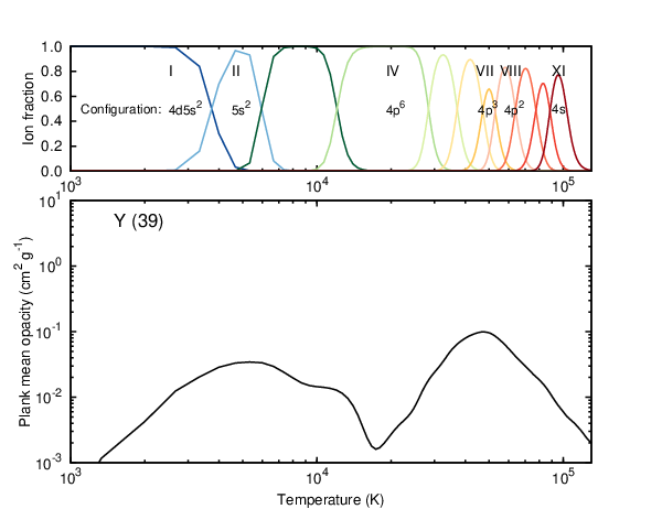
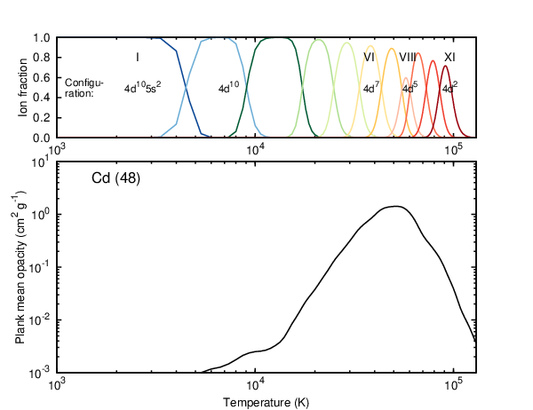
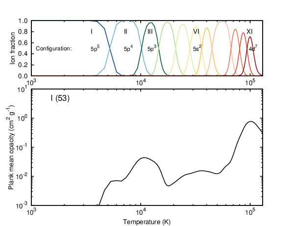
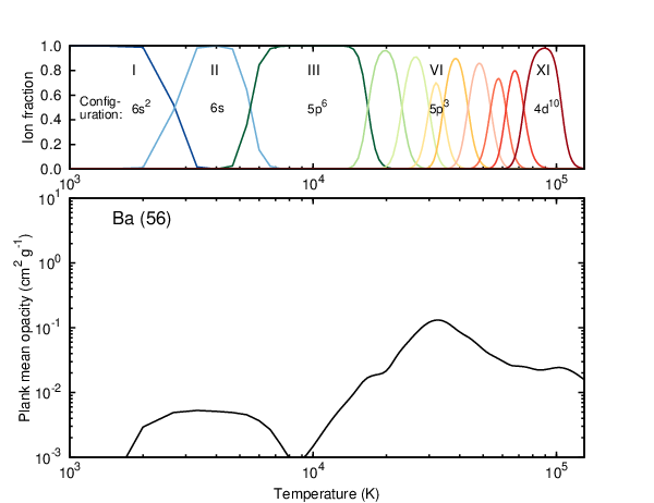
Since the overall variation of the mean opacity is different for each element, we first discuss the trend for a few representative elements from different shells (Figure 3). There are two main factors that determine the trend of opacity for highly ionized ions: half-closed shells have the highest complexity measure, and the increment in in a shell raises the energy distribution upwards (Tanaka et al. 2020). The Boltzmann statistics predicts that lower energy levels are more populated and the transitions from such levels contribute to the opacity the most. At moderate temperatures, the elements or ions with half-closed shells do not necessarily have the highest opacity because their energy levels are pushed toward higher energies. At higher temperatures, higher energy levels are more populated and the opacities of the ions with half-closed shell are greater than other elements within the same shell.
As the ionization degree of -shell element Yttrium (Y, = 39) increases with temperature, the Planck mean opacity evolves as shown in top left panel of Figure 3. When Y is singly or doubly ionized (II III) at K, it has a similar energy level distribution to the neutral -shell elements Strontium (Sr, = 38) and Rubidium (Rb, = 37). These elements contain only a few strong transitions. When Y becomes triply ionized (IV), it has a closed -shell and the opacity decreases. As Y is ionized further, up to V VI, the shell configuration resembles neutral -shell elements () with an energy level distribution at a higher energy. The opacity peaks when Yttrium is sextuply ionized (VII) at K, at which it has a similar structure to neutral Arsenic (As, = 33), with a half-closed shell structure. Beyond this ionization (VIII XI), Y becomes similar to the neutral () and () shell elements. This leads to a decrease in the number of available energy levels, consequently reducing the opacity.
The behavior of the -shell element Cadmium (Cd, 48) is more straightforward (top right panel of Figure 3). As the temperature increases, it loses -shell electrons. When the -shell has a half-closed structure, the element reaches peak opacity. Then, the opacity decreases as more -shell electrons are lost at higher temperature.
The -shell element Iodine (I, = 53) has a complicated variation in opacity with the temperature but can be explained in a similar way (bottom left panel of Figure 3). The opacity is high when I resembles elements with half-closed shells. Namely, the opacity peaks at K and at K, when I has a similar structure to the neutral -shell element Antimony (Sb, = 51) and -shell element Technetium (Te, = 43) respectively, being doubly (III) and tenth (XI) ionized.
For the -shell element Barium (Ba, = 56, bottom right panel of Figure 3), the opacity reaches a peak at K, when Ba is singly ionized (II) and has one neutral electron, similar to Caesium (Cs, = 55). The opacity drops to a negligible value at K, when doubly ionized Ba (III) resembles the energy level distribution of neutral -shell element Xenon (Xe, = 54), which has a closed -shell. Such ions have most of their energy levels distributed at higher energies, and thus fewer transitions take place as the Boltzmann statistics predicts most electrons exist in the lower-lying energy levels at this temperature range. The opacity rises to a higher value at K when the energy distribution is similar to the half-closed neutral -shell element Sb ( = 51). As the ionization degree increases, the opacity decreases again when Ba resembles the configuration of neutral -shell elements with lower complexity.
The variation of the Planck mean opacity with temperature for all the elements of interest can be understood in the same manner (Figure 4). With the increasing temperature and ionization, the effective shell structure of the ions change, the opacity varying accordingly. Highly ionized elements have the maximum bound-bound opacities when they have a half-closed shell structure.
For -shell elements, opacity as a function of temperature peaks when it has half-closed -shell or half-closed -shell structures. The peak opacity is higher when the element has a half-closed -shell structure () rather than a half-closed -shell structure (). Most of the -shell elements have -shell electrons at high ionization, with the opacity peaking at . This is the reason why at early times (higher temperature), -shell elements have comparable opacity contributions to -shell elements.
The -shell elements have comparatively lower opacity . This lower opacity can be explained by -shell elements never resembling neutral half d-shell elements at higher ionization, although they can be similar to neutral half p-shell elements.
The behavior of opacity and temperature for different elements is summarized in Figure 5. At lower temperatures, the elements with the maximum number of low-lying energy levels have the maximum opacity. At high temperatures, ions lose their initial outermost electrons and effectively have different shell structures. Furthermore, the higher-level transitions become attainable at high temperatures since higher energy levels are populated. In this case, the maximum contribution to the opacity typically comes from ions which have half-closed shells, with the highest complexity measure.


|
III.2.2 Opacity of element mixture
In this section, we consider the bound-bound opacities in the ejecta that consist of a mixture of different elements. Depending on the electron fraction , a different abundance pattern is realized in the ejecta. To estimate the bound-bound opacity for blue kilonova, we calculate the opacity for the mixture of elements in an ejecta, assuming . We take the abundance pattern using the results from Wanajo et al. 2014. We assume that the mass distribution in the each bin is flat. At such high , the second and third peak -process elements are not synthesized. The elements with a significant abundance are (Figure 6).
The left panel of Figure 7 shows the expansion opacity as a function of wavelength for the element mixture at 0.1 and 1 day. To model the typical conditions at these times, we set , K for 0.1 day; , K for 1 day. At 1 day, the expansion opacity peaks at , whereas the peak expansion opacity at 0.1 day only reaches . The Planck mean opacity also shows an increase with time (right panel of Figure 7). The value of opacity is for the typical conditions at 0.1 day; under the typical conditions at 1 day, . These results can be understood using Equation 6. Since the expansion opacity is inversely proportional to , the change in from 0.1 to 1 day increases the opacity by a factor of 100. Meanwhile, the Sobolev optical depth decreases with time, which reduces the contribution from the summation of . As a result, the opacity increases by a factor of about 10 as time increases from 0.1 to 1 day.
The Planck mean opacity results for an element mixture as a function of temperature (right panel of Figure 7) can be understood by individual element properties. At relatively low temperatures ( K), the opacity increases with temperature. This is a property of -shell elements that have the largest contribution to the opacity in this temperature range. The opacity displays some modulation by reflecting the behaviors of abundant individual elements. At high temperatures ( K), the opacity evolves more smoothly with temperature because the contributions from - and -shell elements with different peak positions in the Planck mean opacity are averaged out.
Hence, as evidenced by the results, the bound-bound opacity is orders of magnitude greater than the electron scattering, bound-free and free-free opacities. At 0.1 day, the Planck mean of bound-bound opacity can reach up to a value of , whereas other contributions to the total opacity, and , are negligible at a wavelength = 1000 Å for (section II). The bound-free opacity is not significant at this time since the fraction of photons with energy beyond the photo-ionization threshold is small (section II). Therefore, we conclude that bound-bound opacity is the most significant component of the total opacity at an early time ( days).
IV Radiative transfer simulations
Using the new atomic data and opacities, we calculate the light curve of blue kilonova using a time-dependent and wavelength-dependent radiative transfer code (Tanaka & Hotokezaka 2013; Tanaka et al. 2014; Tanaka et al. 2017; Kawaguchi et al. 2018). With a given density structure and distribution, the code calculates the light curves and spectra. The radioactive heating rate of -process nuclei is calculated according to , using the results from Wanajo et al. 2014. The photon transfer is calculated by a Monte Carlo method. The time-dependent thermalization factor is adopted from Barnes et al. 2016. The new opacity data enables us to calculate the radiation transfer starting around hour after the merger. We consider the transitions in a wavelength range 100 - 35000 Å. The simulation is performed from 0.03 to 300 days to calculate the light curves. We describe our model in subsection IV.1 and discuss the evolution of opacity in the ejecta in subsection IV.2. Our results for the bolometric luminosity calculation using this opacity is presented in subsection IV.3.
IV.1 Model
We use a simple ejecta model (Metzger et al. 2010) which considers a spherical ejecta expanding homologously. As our fiducial case, we use the power-law density structure from a velocity 0.05c to 0.2c, a total ejecta mass of , and an electron fraction range of 0.30 0.40. Similarly to subsection III.2, we assume a flat distribution of mass for each value in the range, subsequently using the results from Wanajo et al. 2014 to calculate the abundance pattern. Throughout the ejecta, the same distribution, and hence homogeneous elemental abundance pattern, are assumed. The velocity scale and the range of in our fiducial model are typical for disk wind ejecta, particularly in the case of a relatively long-lived hypermassive NS (Perego et al. 2014; Metzger & Fernández 2014; Lippuner et al. 2017; Siegel & Metzger 2017; Fujibayashi et al. 2018; Fernández et al. 2019). In such conditions, the main nucleosynthesis products are light -process elements (Figure 6).
In reality, the disk wind ejecta are enveloped inside a faster moving dynamical ejecta (Hotokezaka et al. 2013). To study the effect of this dynamical ejecta, we further include models with a continuous thin outer layer at with a fixed mass of . The layer has a steeper density structure where , and . According to the slope, the maximum outer velocity changes as 0.24c, 0.25c, and 0.33c, for , and , respectively. We assume the same range for these outer ejecta components. These modelling conditions may be applicable for a shock-heated polar dynamical ejecta, where can rise by capture and absorption (Goriely et al. 2015; Sekiguchi et al. 2015; Sekiguchi et al. 2016; Martin et al. 2018; Radice et al. 2018). Thus, even with relatively high , our model can provide a sound approximation for the emission viewed from the polar direction. We do not include lanthanide-rich ejecta as the main focus of this work is to present the light curves of blue kilonovae.
IV.2 Evolution of opacity
As the ejecta expands, the temperature and the density of the ejecta decrease. The opacity also evolves with time accordingly. Therefore, it is useful to study the time evolution of the opacities at a fixed position in the ejecta. Figure 8 shows the temperature, density and opacity evolution at the ejecta point for our fiducial model. The dominant component is the bound-bound opacity, followed by the electron-scattering, bound-free, and free-free opacity. The total opacity varies from 0.1 10 with time.
The contribution of electron scattering to the total opacity is higher at earlier times, reaching a majority contribution, , at 1 hour (Figure 8). This high electron scattering contribution occurs at an early time as high temperatures ( K) cause a high degree of ionization, which raises electron density. The electron scattering opacity decreases with time as the ejecta temperature decreases. Around days, the electron scattering contribution drops steeply because most of the elements recombine to neutral atoms.
The free-free component remains small throughout the evolution of the total opacity. At day, the opacity has a value of ; this value falls faster than the electron scattering opacity component as time increases.


(Figure 8). From Equation 3 and Equation 4, we can see that the free-free opacity varies as . Since the density decreases faster than temperature as time increases, the free-free opacity decreases with time.
The bound-free opacity varies with time but never becomes large enough to significantly contribute to the total opacity. As discussed in subsection II.3, although the photo-ionization cross section itself is high, the fraction of high energy photons is small, and thus, the Planck mean opacity is moderate. The bound-free opacity component shows an increasing trend, reaching its peak value of a few days after the merger. This is as a result of the ionization degree decreasing with time, hence more photons are present beyond the potential energy of ions. It should be noted that the value of the bound-free opacity before = 0.2 day is not correctly followed in the radiative transfer code, since the wavelength range beyond the ionization threshold is not covered by our wavelength grid (down to 100 Å).
The bound-bound opacity component evolves from to from 0.1 to 1 day. Excluding the time around 1 hour, this component alone is representative of the total opacity. It is to be noted that most of the previous works have considered a fixed opacity value of 1 or less (Kasliwal et al. 2017; Villar et al. 2017; Piro & Kollmeier 2018; Gottlieb & Loeb 2020) to calculate blue kilonovae at day. This assumption is not valid precisely, as the change in the opacity with time is quite large for even high ejecta.
IV.3 Bolometric light curves
The bolometric luminosity for the fiducial model is shown in Figure 9. The luminosity deposited the ejecta (or thermalized radioactive luminosity) is shown by the dashed line for comparison. At 1 day, the observable bolometric luminosity is an order of magnitude lower than the deposition luminosity because the ejecta are optically thick, hence photons cannot escape from the ejecta. At 1 day, the previously stored radiation energy from 1 day starts to be released and the bolometric luminosity supersedes the deposition luminosity. Finally, the bolometric luminosity follows the thermalized radioactive emission at 10 days.
The bolometric light curve of GW170817 (Waxman et al. 2018) is shown for comparison. Our fiducial model with gives a reasonable agreement with the observed data at early times. The required ejecta mass is consistent with the findings of previous works (Kasliwal et al. 2017; Waxman et al. 2018; Hotokezaka & Nakar 2020).
The presence of a thin outer layer affects the light curves at an early time (Figure 10). The steeper slope of the outer ejecta makes the luminosity fainter at 1 day. In the early time, the ejecta are optically thick and the emission from the outermost layer determines the light curve. Adding a thin outer layer to the ejecta changes the mass located outside of the diffusion sphere in the early time. Our fiducial model has a higher density at the diffusion sphere, producing a high luminosity in the early time (Figure 10). For the models with thin layers, the density at the diffusion sphere becomes lower. Since the model with a steeper slope has a lower density of the optically thin layer for a fixed mass of the outer ejecta, the model displays a fainter luminosity. After around day, the thin layer has almost no effect on the light curve because thin ejecta are already optically thin and so do not contribute to the luminosity anymore.


|
V Discussions
V.1 Applications to GW170817
The spectra at and 10 days after the merger, and the multi-color light curves, both plotted in absolute magnitude, are shown for the fiducial model (left and right panel in Figure 11). The spectral shape shows a strong time evolution from shorter wavelengths ( 10000 Å ) towards infrared wavelengths ( Å) at later times. This trend is also displayed in the multi-color light curves. The peak times of the light curves gradually move from shorter to longer wavelengths: the UV light curves peak at 4.3 hours, blue optical light curves peak at 16.8 hours, and red optical and NIR light curves peak at 1 day. The early UV emission declines very quickly and becomes fainter than an absolute magnitude of in 2 days. A similar pattern for blue optical emission occurs over a somewhat longer timescale. The NIR brightness remains bright from 1 day to a week.
We compare our model with the multi-color light curves of GW170817 (Villar et al. 2017). The data are corrected for Galactic extinction with . This comparison provides insight on the emission mechanism of GW170817-like events. Similar to the bolometric luminosity (Figure 9), our fiducial model shows reasonable agreement with the data. Hence, our model shows that a one-component, purely-radioactive, high ejecta can explain early-time bright UV and blue emission. Previous studies that assumed a constant opacity also show good agreement for early UV and blue optical data Cowperthwaite et al. 2017; Drout et al. 2017; Kasen et al. 2017; Villar et al. 2017. However, our calculations directly calculate atomic opacities, and thus, the opacity is not a free parameter in our model.
The UV magnitudes become fainter and decline faster upon the inclusion of a thin layer outside the fiducial model ejecta (Figure 12); also pointed out by Kasen et al. 2017. The UV light curves are shown for the fiducial model and the case where . The UVW1 magnitude of the fiducial model without a thin layer peaks at an absolute magnitude of mag at hours, whereas that of the model incorporating a thin layer with is fainter at day, reaching a peak of mag at hours.
It should be noted that our models assume that the outer ejecta are lanthanide-free, with . If the outer ejecta have a lower , as expected for dynamical ejecta in the equatorial plane, the UV brightness can be suppressed further. Hence, the purely radioactive kilonova models may not be able to explain the observed early light curve, depending on the structure and composition of the outer ejecta. In this case, a heating source other than radioactive decays of -process nuclei may be necessary, for example, heating by shock or cocoon (Kasliwal et al. 2017; Piro & Kollmeier 2018), decay luminosity from free neutrons (Metzger et al. 2015; Gottlieb & Loeb 2020), or some other central power source (Metzger et al. 2008; Yu et al. 2013; Metzger & Fernández 2014; Matsumoto et al. 2018; Metzger et al. 2018; Li et al. 2018; Wollaeger et al. 2019). Although it is difficult to draw firm conclusions due to a lack of atomic data on highly-ionized lanthanides, our new atomic opacities provide the foundation for a discussion on the detailed properties of blue kilonova models at an early phase.
V.2 Future prospects


|
Finally, we discuss the prospect of observing an early kilonova emission. Our simulations give the first synthetic light curves of kilonova at a timescale of hours after the merger, based on the detailed atomic opacities. As discussed in subsection V.1, the early UV emission is sensitive to the structure of the ejecta. Furthermore, contributions from other heating sources may play important roles determining the early luminosity. Therefore, the early-time observations provide clues to distinguish these models.
Although the first UVOIR data of GW170817 were obtained at 11 hours, the early data suggest that UV and blue optical emissions peak before this time. In our fiducial model, UVW1 and optical -band magnitudes peak at 4.3 hours and 16.8 hours respectively (Figure 11). When the ejecta is enveloped by a thin outer layer, with a density slope , the UVW1 magnitude peaks earlier, reaching a value of mag at 2.4 hours (Figure 12). Figure 13 shows the expected observed magnitudes in UV and optical -band at 200 Mpc. The UVW1 and -band magnitudes at 200 Mpc reach apparent magnitudes of 20.5 and 19.8 mag, respectively at the peak time.
The early UV signals are bright enough to be detected by existing facilities like Swift (Roming et al. 2005), which has a limiting magnitude of 22 mag for an exposure time of 1000 s (Brown et al. 2014), if a counterpart is discovered early enough to start UV observations promptly. A more promising detection method is via wide-field survey observations in the UV wavelengths, as UV emissions peak earlier than optical emissions. Upcoming wide field surveys, such as those carried out by the Ultraviolet Transient Astronomy Satellite (ULTRASAT, Sagiv et al. 2014), which can detect down to the AB magnitude of about 22.4 mag in 900 s, are able to detect the expected signal from our fiducial model even at 500 Mpc distance.
VI Conclusions
In this paper, we have calculated the atomic structures and opacities for the elements with atomic number of , which are necessary to understand the properties of early blue kilonova from NS mergers. We cover ionizations up to the tenth degree (XI) at a typical ejecta temperature at days ( K). We find that the bound-bound opacities are the dominant source of the opacity at early times ( day). Among different elements and ionization states, ions with half-closed electron shells provide the highest contributions to the bound-bound opacity. The Planck mean opacity of the lanthanide-free ejecta at early times is about one order of magnitude lower than the opacity at late times: at 0.1 day, compared to at 1 day.
Using this opacity, we have performed multi-wavelength radiative transfer simulations and calculated the bolometric and multi-color light curves of blue kilonova. Our fiducial model, with an ejecta mass of , reaches the bolometric luminosity of by days. The UV and blue optical band magnitudes reach their peak absolute magnitudes of mag and mag at 4.3 and 16.8 hours, respectively. The behaviors of early light curves are affected by the outer structure of the ejecta. The presence of a thin outer layer greatly suppresses the luminosity at 1 day, agreeing with the results of Kasen et al. 2017. The comparison of our fiducial model with the bolometric and multi-color light curves of GW170817 in the early phase shows reasonable agreement. Our result suggests that the early data of GW170817 can be explained with a purely radioactive kilonova model with a high ejecta.
However, there are some limitations of our models. Firstly, we have considered only high , lanthanide-free outer ejecta. As the low , lanthanide-rich ejecta can have quite different properties of opacities, which in turn affect the luminosity, we cannot yet firmly exclude the possibility of a heating source other than radioactive heating at early times. Moreover, we did not take into account the multi-dimensional, multi-component ejecta, as considered by e.g., Villar et al. 2017, Perego et al. 2017, and Kawaguchi et al. 2018. These assumptions prevent us from precisely predicting the emission viewed from the equatorial region, where the presence of the lanthanide-rich, dynamical ejecta is expected.
Despite these limitations, our model will be helpful in quantitatively comparing the models with future early-time observations for NS merger events. Our model predicts bright early-time UV emission that is detectable with the Swift satellite at a distance of 200 Mpc, if observations are started promptly. Furthermore, wide-field UV surveys with upcoming satellites such as ULTRASAT can detect such emissions, even at distances as large as 500 Mpc. Such early UV observations will provide rich information about the structure of the outermost ejecta, providing a unique way to test the presence of other heating sources such as a cocoon, decays of free neutrons, or a long-lived central engine.
References
- Abbott et al. (2017) Abbott, B. P., Abbott, R., Abbott, T. D., et al. 2017, Phys. Rev. Lett., 119, 161101, doi: 10.1103/PhysRevLett.119.161101
- Arcavi (2018) Arcavi, I. 2018, ApJ letters, 855, L23. https://arxiv.org/abs/1802.02164
- Bar-Shalom et al. (2001) Bar-Shalom, A., Klapisch, M., & Oreg, J. 2001, J. Quant. Spec. Radiat. Transf., 71, 169, doi: 10.1016/S0022-4073(01)00066-8
- Barnes et al. (2016) Barnes, J., Kasen, D., Wu, M.-R., & Martínez-Pinedo, G. 2016, ApJ, 829, 110, doi: 10.3847/0004-637X/829/2/110
- Brown et al. (2014) Brown, P. J., Breeveld, A. A., Holland, S., Kuin, P., & Pritchard, T. 2014, Ap&SS, 354, 89, doi: 10.1007/s10509-014-2059-8
- Connaughton et al. (2017) Connaughton, V., Goldstein, A., & Fermi GBM - LIGO Group. 2017, in American Astronomical Society Meeting Abstracts, Vol. 229, American Astronomical Society Meeting Abstracts #229, 406.08
- Coulter et al. (2017) Coulter, D. A., Foley, R. J., Kilpatrick, C. D., et al. 2017, Science, 358, 1556, doi: 10.1126/science.aap9811
- Cowperthwaite et al. (2017) Cowperthwaite, P. S., Berger, E., Villar, V. A., et al. 2017, ApJ, 848, L17, doi: 10.3847/2041-8213/aa8fc7
- Drout et al. (2017) Drout, M. R., Piro, A. L., Shappee, B. J., et al. 2017, Science, 358, 1570, doi: 10.1126/science.aaq0049
- Eastman & Pinto (1993) Eastman, R. G., & Pinto, P. A. 1993, ApJ, 412, 731, doi: 10.1086/172957
- Eichler et al. (1989) Eichler, D., Livio, M., Piran, T., & Schramm, D. N. 1989, Nature, 340, 126, doi: 10.1038/340126a0
- Evans et al. (2017) Evans, P. A., Cenko, S. B., Kennea, J. A., et al. 2017, Science, 358, 1565, doi: 10.1126/science.aap9580
- Fernandez & Metzger (2014) Fernandez, R., & Metzger, B. 2014, in AAS/High Energy Astrophysics Division #14, AAS/High Energy Astrophysics Division, 304.07
- Fernández et al. (2019) Fernández, R., Tchekhovskoy, A., Quataert, E., Foucart, F., & Kasen, D. 2019, MNRAS, 482, 3373, doi: 10.1093/mnras/sty2932
- Fontes et al. (2020) Fontes, C. J., Fryer, C. L., Hungerford, A. L., Wollaeger, R. T., & Korobkin, O. 2020, MNRAS, 493, 4143, doi: 10.1093/mnras/staa485
- Fontes et al. (2017) Fontes, C. J., Fryer, C. L., Hungerford, A. L., et al. 2017, arXiv e-prints, arXiv:1702.02990. https://arxiv.org/abs/1702.02990
- Freiburghaus et al. (1999) Freiburghaus, C., Rosswog, S., & Thielemann, F. K. 1999, ApJ, 525, L121, doi: 10.1086/312343
- Fujibayashi et al. (2018) Fujibayashi, S., Kiuchi, K., Nishimura, N., Sekiguchi, Y., & Shibata, M. 2018, ApJ, 860, 64, doi: 10.3847/1538-4357/aabafd
- Gaigalas et al. (2019) Gaigalas, G., Kato, D., Rynkun, P., Radžiūtė, L., & Tanaka, M. 2019, ApJS, 240, 29, doi: 10.3847/1538-4365/aaf9b8
- Goriely et al. (2015) Goriely, S., Bauswein, A., Just, O., Pllumbi, E., & Janka, H. T. 2015, MNRAS, 452, 3894, doi: 10.1093/mnras/stv1526
- Gottlieb & Loeb (2020) Gottlieb, O., & Loeb, A. 2020, MNRAS, 493, 1753, doi: 10.1093/mnras/staa363
- Hallinan et al. (2017) Hallinan, G., Corsi, A., Mooley, K. P., et al. 2017, Science, 358, 1579, doi: 10.1126/science.aap9855
- Hotokezaka et al. (2013) Hotokezaka, K., Kiuchi, K., Kyutoku, K., et al. 2013, Phys. Rev. D, 88, 044026, doi: 10.1103/PhysRevD.88.044026
- Hotokezaka & Nakar (2020) Hotokezaka, K., & Nakar, E. 2020, ApJ, 891, 152, doi: 10.3847/1538-4357/ab6a98
- Karp et al. (1977) Karp, A. H., Lasher, G., Chan, K. L., & Salpeter, E. E. 1977, ApJ, 214, 161, doi: 10.1086/155241
- Kasen et al. (2013) Kasen, D., Badnell, N. R., & Barnes, J. 2013, ApJ, 774, 25, doi: 10.1088/0004-637X/774/1/25
- Kasen et al. (2017) Kasen, D., Metzger, B., Barnes, J., Quataert, E., & Ramirez-Ruiz, E. 2017, Nature, 551, 80, doi: 10.1038/nature24453
- Kasliwal et al. (2017) Kasliwal, M. M., Nakar, E., Singer, L. P., & et al. 2017, Science, 358, 1559, doi: 10.1126/science.aap9455
- Kawaguchi et al. (2018) Kawaguchi, K., Shibata, M., & Tanaka, M. 2018, ApJ letter, 865, L21. https://arxiv.org/abs/1806.04088
- Korobkin et al. (2012) Korobkin, O., Rosswog, S., Arcones, A., & Winteler, C. 2012, MNRAS, 426, 1940, doi: 10.1111/j.1365-2966.2012.21859.x
- Kramida et al. (2018) Kramida, A., Ralchenko, Y., Reader, J., & NIST ASD Team. 2018, NIST Atomic Spectra Database (version 5.6.1), https://physics.nist.gov/asd. National Institute of Standards and Technology, Gaithersburg, MD.
- Kulkarni (2005) Kulkarni, S. R. 2005, arXiv e-prints, astro. https://arxiv.org/abs/astro-ph/0510256
- Lattimer & Schramm (1974) Lattimer, J. M., & Schramm, D. N. 1974, ApJ, 192, L145, doi: 10.1086/181612
- Li & Paczyński (1998) Li, L.-X., & Paczyński, B. 1998, ApJ, 507, L59, doi: 10.1086/311680
- Li et al. (2018) Li, S.-Z., Liu, L.-D., Yu, Y.-W., & Zhang, B. 2018, The Astrophysical Journal, 861, L12, doi: 10.3847/2041-8213/aace61
- Lippuner et al. (2017) Lippuner, J., Fernández, R., Roberts, L. F., et al. 2017, MNRAS, 472, 904, doi: 10.1093/mnras/stx1987
- Martin et al. (2018) Martin, D., Perego, A., Kastaun, W., & Arcones, A. 2018, Classical and Quantum Gravity, 35, 034001, doi: 10.1088/1361-6382/aa9f5a
- Matsumoto et al. (2018) Matsumoto, T., Ioka, K., Kisaka, S., & Nakar, E. 2018, ApJ, 861, 55, doi: 10.3847/1538-4357/aac4a8
- Metzger et al. (2015) Metzger, B. D., Bauswein, A., Goriely, S., & Kasen, D. 2015, MNRAS, 446, 1115, doi: 10.1093/mnras/stu2225
- Metzger & Fernández (2014) Metzger, B. D., & Fernández, R. 2014, MNRAS, 441, 3444, doi: 10.1093/mnras/stu802
- Metzger et al. (2008) Metzger, B. D., Piro, A. L., & Quataert, E. 2008, MNRAS, 390, 781, doi: 10.1111/j.1365-2966.2008.13789.x
- Metzger et al. (2018) Metzger, B. D., Thompson, T. A., & Quataert, E. 2018, ApJ, 856, 101, doi: 10.3847/1538-4357/aab095
- Metzger et al. (2010) Metzger, B. D., Martínez-Pinedo, G., Darbha, S., et al. 2010, MNRAS, 406, 2650, doi: 10.1111/j.1365-2966.2010.16864.x
- Mooley & Mooley (2017) Mooley, K. P., & Mooley, S. 2017, GRB Coordinates Network, 22211, 1
- Perego et al. (2017) Perego, A., Radice, D., & Bernuzzi, S. 2017, ApJ, 850, L37, doi: 10.3847/2041-8213/aa9ab9
- Perego et al. (2014) Perego, A., Rosswog, S., Cabezón, R. M., et al. 2014, MNRAS, 443, 3134, doi: 10.1093/mnras/stu1352
- Pinto & Eastman (2000) Pinto, P. A., & Eastman, R. G. 2000, arXiv e-prints, astro. https://arxiv.org/abs/astro-ph/0006171
- Piro & Kollmeier (2018) Piro, A. L., & Kollmeier, J. A. 2018, ApJ, 855, 103, doi: 10.3847/1538-4357/aaaab3
- Radice et al. (2018) Radice, D., Perego, A., Hotokezaka, K., et al. 2018, ApJ, 869, 130, doi: 10.3847/1538-4357/aaf054
- Radžiūtė et al. (2020) Radžiūtė, L., Gaigalas, G., Kato, D., Rynkun, P., & Tanaka, M. 2020, arXiv e-prints, arXiv:2002.08075. https://arxiv.org/abs/2002.08075
- Roberts et al. (2011) Roberts, L. F., Kasen, D., Lee, W. H., & Ramirez-Ruiz, E. 2011, ApJ, 736, L21, doi: 10.1088/2041-8205/736/1/L21
- Roming et al. (2005) Roming, P. W. A., Kennedy, T. E., Mason, K. O., et al. 2005, Space Sci. Rev., 120, 95, doi: 10.1007/s11214-005-5095-4
- Rosswog et al. (2018) Rosswog, S., Sollerman, J., Feindt, U., et al. 2018, A&A, 615, A132, doi: 10.1051/0004-6361/201732117
- Rybicki & Lightman (1986) Rybicki, G. B., & Lightman, A. P. 1986, Radiative Processes in Astrophysics
- Sagiv et al. (2014) Sagiv, I., Gal-Yam, A., Ofek, E. O., et al. 2014, AJ, 147, 79, doi: 10.1088/0004-6256/147/4/79
- Savchenko et al. (2017) Savchenko, V., Ferrigno, C., Kuulkers, E., et al. 2017, in Proceedings of the 7th International Fermi Symposium, 58
- Sekiguchi et al. (2015) Sekiguchi, Y., Kiuchi, K., Kyutoku, K., & Shibata, M. 2015, Phys. Rev. D, 91, 064059, doi: 10.1103/PhysRevD.91.064059
- Sekiguchi et al. (2016) Sekiguchi, Y., Kiuchi, K., Kyutoku, K., Shibata, M., & Taniguchi, K. 2016, Phys. Rev. D, 93, 124046, doi: 10.1103/PhysRevD.93.124046
- Shibata et al. (2017) Shibata, M., Fujibayashi, S., Hotokezaka, K., et al. 2017, Phys. Rev. D, 96, 123012, doi: 10.1103/PhysRevD.96.123012
- Siegel & Metzger (2017) Siegel, D. M., & Metzger, B. D. 2017, Phys. Rev. Lett., 119, 231102, doi: 10.1103/PhysRevLett.119.231102
- Tanaka & Hotokezaka (2013) Tanaka, M., & Hotokezaka, K. 2013, ApJ, 775, 113
- Tanaka et al. (2014) Tanaka, M., Hotokezaka, K., Kyutoku, K., & et al. 2014, ApJ, 780, 31. https://arxiv.org/abs/1310.2774
- Tanaka et al. (2018) Tanaka, M., Kato, D., Gaigalas, G., & et al. 2018, ApJ, 852, 109. https://arxiv.org/abs/1708.09101
- Tanaka et al. (2020) Tanaka, M., Kato, D., Gaigalas, G., & Kawaguchi, K. 2020, MNRAS, 496, 1369, doi: 10.1093/mnras/staa1576
- Tanaka et al. (2017) Tanaka, M., Utsumi, Y., Mazzali, P. A., & et al. 2017, PASJ, 69, 102. https://arxiv.org/abs/1710.05850
- Troja et al. (2017) Troja, E., Piro, L., van Eerten, H., et al. 2017, Nature, 551, 71, doi: 10.1038/nature24290
- Valenti et al. (2017) Valenti, S., Sand, D. J., Yang, S., et al. 2017, ApJ, 848, L24, doi: 10.3847/2041-8213/aa8edf
- Verner et al. (1996) Verner, D. A., Ferland, G. J., Korista, K. T., & Yakovlev, D. G. 1996, ApJ, 465, 487, doi: 10.1086/177435
- Villar et al. (2017) Villar, V. A., Guillochon, J., Berger, E., et al. 2017, ApJ, 851, L21, doi: 10.3847/2041-8213/aa9c84
- Wanajo et al. (2014) Wanajo, S., Sekiguchi, Y., Nishimura, N., & et al. 2014, ApJ, 789, L39, doi: 10.1088/2041-8205/789/2/L39
- Waxman et al. (2018) Waxman, E., Ofek, E. O., Kushnir, D., & Gal-Yam, A. 2018, MNRAS, 481, 3423, doi: 10.1093/mnras/sty2441
- Wollaeger et al. (2017) Wollaeger, R. T., Hungerford, A. L., Fryer, C. L., et al. 2017, ApJ, 845, 168, doi: 10.3847/1538-4357/aa82bd
- Wollaeger et al. (2019) Wollaeger, R. T., Fryer, C. L., Fontes, C. J., et al. 2019, ApJ, 880, 22, doi: 10.3847/1538-4357/ab25f5
- Yang et al. (2017) Yang, S., Valenti, S., Cappellaro, E., et al. 2017, ApJ, 851, L48, doi: 10.3847/2041-8213/aaa07d
- Yu et al. (2013) Yu, Y.-W., Zhang, B., & Gao, H. 2013, ApJ, 776, L40, doi: 10.1088/2041-8205/776/2/L40