It is our goal to establish that a weak gravity condition and stringy states in the gravity sector emerge naturally when one couples theories of metastable HS particles to gravity. So, first we define exactly what we mean by theories of metastable HS particles and the ‘gravity sector’.

First, consider a non-gravitational QFT which may contain both low spin and HS particles $\{G_{J}\}$. We assume that this theory has a consistent S-matrix. This immediately implies that all particles in this theory with spin $J\geq 3$ must be massive [17, 18]. Furthermore, we assume that the particles $\{G_{J}\}$ are approximately elementary from an effective field theory perspective (see figure 1 for a pictorial depiction). This can be restated in the following way. Below some cut-off scale $\Lambda_{\rm QFT}\gg m_{J}$, where $m_{J}$’s are the masses of $G_{J}$ particles,

• (i) particles $\{G_{J}\}$ represent all the degrees of freedom of the theory,

• (ii) $G_{J}$ particles are metastable, so all effective low-energy couplings between low-energy particles are small.

For example, all three-point interactions

must be suppressed: $|\lambda|\ll 1$.³³ 3 We also assume that the kinetic mixings between different $G_{J}$-particles are small. Thus, the S-matrix in this theory is a meromorphic function with simple poles only at the location of $\{G_{J}\}$ particles. Of course, the S-matrix must also be consistent with unitarity, causality, and crossing symmetry.

So, particles in the $\{G_{J}\}$-sector can be free or weakly interacting below the energy scale $\Lambda_{\rm QFT}$. In general, a $G_{J}$ particle can interact with itself by exchanging one or multiple particles from the $\{G_{J}\}$-sector, as shown in figure 2. We parametrize the strength of this interaction by $g_{J}\sim\lambda$. This dimensionless parameter will play an important role when we include gravity.

We will eventually couple the above theory to a gravity sector. We assume that the particles $\{G_{J}\}$ remain effectively elementary below the energy scale $\Lambda_{\rm QFT}$ even when we couple the theory to gravity. Hence, the S-matrix in the resulting theory still is a meromorphic function with simple poles which are now located at the position of $\{G_{J}\}$ particles, the graviton $h_{\mu\nu}$, and other particles in the gravity sector (if any). A $G_{J}$ particle can decay into two gravitons, however, we impose the following restriction.

• (iii) $G_{J}$ particles are gravitationally metastable: the three-point interactions

  $$\langle G_{J}hh\rangle\sim\frac{\lambda_{G}}{M_{\rm pl}^{2}}$$

  (1.2)

  are not too large $\lambda_{G}\sim{\cal O}(1)$.⁴⁴ 4 This condition is violated by bound states in gauge theories at large $N$. In certain situations this assumption can be relaxed. We will discuss this in more detail in section 3.

We will distinguish between two classes of consistent theories with such HS particles. (A) A theory with finite number of HS particles which are weakly coupled, unitary, and causal up to the energy scale $\Lambda_{\rm QFT}\gg m_{J}$. For example, massive free HS particles belong in this class. (B) A theory with an infinite number of HS particles with unbounded spin. This scenario necessarily requires $\Lambda_{\rm QFT}=\infty$, since a thermodynamically healthy theory should not have an accumulation point in the spectrum. Tree-level open string theory belongs in this class. Clearly, there is some overlap between class A and class B theories. If we integrate out all states in a class B theory above some $\Lambda_{\rm QFT}$, we obtain an effective field theory of HS particles which is in class A. However, not all class A theories come from class B theories. For example, a class A theory can come from a strongly coupled UV complete theory.

We assume that the gravitational sector is consistent on its own, and may contain other particles. To be precise, let us consider a $G_{J}G_{J}\rightarrow G_{J}G_{J}$ scattering for an arbitrary $G_{J}$. In the limit $M_{\rm pl}\rightarrow\infty$, the tree-level scattering amplitude is a meromorphic function with simple poles only at the location of $\{G_{J}\}$ particles. When $M_{\rm pl}$ is large but finite, the same scattering amplitude must develop at least one more simple pole corresponding to the graviton. In addition, the scattering amplitude may develop additional simple poles which only disappear in the strict limit of $M_{\rm pl}\rightarrow\infty$. These extra poles represent other particles in the gravity sector. Next, we will argue that these additional gravitational poles are essential to the preservation of causality.

We will argue that the $G_{J}$-particles cannot couple to gravity while preserving causality unless there exist HS states⁵⁵ 5 These cannot simply be a tower of other $G_{J}$-particles within the non-gravitational sector. in the gravitational sector. Furthermore, we derive a bound on the mass $\Lambda_{\rm gr}$ of the lightest HS particle in the gravity sector in terms of $g_{J}$, $m_{J}$, and $M_{\rm pl}$. In particular, in $(3+1)$-dimensions even a conservative estimate implies that $\Lambda_{\rm gr}$ must be small enough such that

for all $J\geq 3$ particles. Hence, in general there can be a parametric separation between $\Lambda_{\rm gr}$ and $m_{\rm min}$. The optimal bound is obtained for the particle in the $\{G_{J}\}$-sector that minimizes the right hand side of (1.2). Of course, the above bound is only a necessary condition but it may be far from being sufficient. For example, for any theory of finite number of elementary HS particles (equivalently type A with $\Lambda_{\rm QFT}=\infty$) causality requires $\Lambda_{\rm gr}\lesssim m_{\rm min}$ even if all HS particles satisfy $|g_{J}|\gtrsim\frac{m_{J}}{M_{\rm pl}}$, where $m_{\rm min}$ is the mass of the lightest HS particle in the $\{G_{J}\}$-sector.

The above bound is closely related to the weak gravity conjecture [19, 20] (for a recent review see [21]). It is also reminiscent of the higher spin swampland conjecture of [22]. Consider a theory of stable or metastable HS particles coupled to gravity in 4d. The theory, as we stated before, must contain gravitational states at or below $\Lambda_{\rm gr}$. However, we can still obtain a low energy QFT description for a set of light HS particles by integrating out states above $\Lambda_{\rm gr}$. Hence, a QFT description exists for a HS particle of mass $m_{J}$ and interaction strength $g_{J}$ only when $\Lambda_{\rm gr}\gg m_{J}$. The bound (1.2) implies that the QFT approximation necessarily breaks down when $|g_{J}|\lesssim\frac{m_{J}}{M_{\rm pl}}$. This is precisely the statement that the non-gravitational interaction between the particles is weaker than the gravitational interaction. We will also argue that such a particle must have stringy scattering amplitudes.

These ideas are motivated by recent work [9] that greatly curtails the existence of stable higher-spin particles $G_{J}$. We can break our main argument into three steps, which we work through in detail in section 3. Here is a brief outline:

1. 1.

   HS particles $G_{J}$ have 3-pt couplings to the graviton $h$ that are highly constrained. There is a unique structure for the $G_{J}G_{J}h$ vertex in $D=4$ dimensions that allows a tree-level $G_{J}h\to G_{J}h$ scattering to proceed above the scale of the mass $m_{J}$ of the HS particle without causality violations. Interestingly, this unique structure matches⁶⁶ 6 We thank Simon Caron-Huot for pointing this out to us. the universal coupling [23] of gravitons to Kerr black holes in the classical limit.

2. 2.

   Vertices involving distinct HS particles $G_{J}G_{J^{\prime}}h$ must be suppressed by positive powers of $1/\Lambda_{\rm gr}$, a new scale $\Lambda_{\rm gr}>m_{J},m_{J^{\prime}}$. This follows from causality which implies that the process $G_{J}h\to G_{J^{\prime}}h$ is bounded by the process $G_{J}h\to G_{J}h$. New HS particles must be present in the gravity sector at $\Lambda_{\rm gr}$. However, from this argument alone we cannot constrain $\Lambda_{\rm gr}$, and it would be self consistent to simply set the vertex $G_{J}G_{J^{\prime}}h$ to zero and include no new HS particles. Nevertheless, the fact that all vertices $G_{J}G_{J^{\prime}}h$ are suppressed will play a crucial role in deriving the bound (1.2).

3. 3.

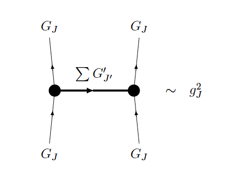
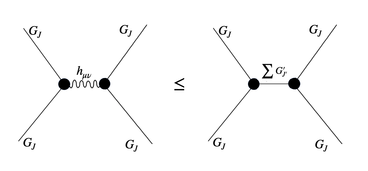
   Finally, we can complete the argument by studying the scattering $G_{J}G_{J}\rightarrow hh$. In this step the main physical point is that this process involves the diagram on the right of figure 3. This can be interpreted as an exchange of $G_{J}$, and so it naively seems to badly violate causality constraints [3] and the chaos bound [24] for $J\geq 3$.⁷⁷ 7 In [11], authors proposed that in any UV complete theory of gravity coincident gravitational shocks should commute. The diagram on the right of figure 3 also appears when one studies commutativity of coincident shocks for HS particles coupled to gravity. Indeed, causality constraints obtained from the first two steps of our argument guarantee that coincident gravitational shocks commute below the energy scale $\Lambda_{\rm gr}$.

   However this conclusion is premature for two reasons: (1) the exchange of an infinite tower $\sum G_{J}$ of other HS particles (in the non-gravitational sector) might resolve the problem, and (2) causality constraints cannot be directly applied because the incoming and outgoing states are different. The first issue with the argument is resolved by the previous step, which showed that $G_{J}G_{J^{\prime}}h$ vertices must be additionally suppressed by $\Lambda_{\rm gr}$, and so these exchanges cannot rescue causality unless the bound (1.2) is satisfied. The second issue can be resolved by studying a scattering experiment involving a coherent superposition of many states of the form $\alpha G_{J}+\beta h$. Now the diagram on the right of figure 3 contributes and coherence guarantees that a 2-to-2 scattering process exists.

   A careful study of this process imposes a bound on the diagram on the right of figure 3. This, in turn, connects the parameters of the non-gravitational theory to the scale $\Lambda_{\rm gr}$ where new HS particles contribute in the gravity sector, bounding $\Lambda_{\rm gr}$ as in equation (1.2).

This argument implies the existence of HS particles in the gravity sector at a scale $\Lambda_{\rm gr}\ll M_{\rm pl}$. As a byproduct, we derive that the gravitational scattering amplitude $G_{J}G_{J}\rightarrow G_{J}G_{J}$ of any HS particle with mass $m_{J}\ll\Lambda_{\rm gr}$ must be smaller than the non-gravitational scattering amplitude of $G_{J}G_{J}\rightarrow G_{J}G_{J}$ in the impact parameter space (see figure 4). It is possible that the connection between causality and the weak gravity conjecture is more general. In fact, this connection was also observed in a wide class of theories [25].

The fact that there can be a parametric separation between $\Lambda_{\rm gr}$ and $m_{J}$ is true only in $D=4$ dimensions. In this sense, 4d is special because it allows for a field theoretic description of HS theories coupled to gravity. For $D>4$, the three-step argument discussed above is not actually needed. The first step alone implies that a theory with approximately elementary HS states in $D>4$ must have new HS states in the gravity sector at or below $m_{\rm min}$.⁸⁸ 8 The CKSZ theorem applies here as well implying any such theory in $D\geq 5$ dimensions only have a stringy description. On the other hand, in 3d there are non-string theory models with infinite number of interacting massive higher spin fields [26, 27].

Theories of HS particles are known to be highly constrained [28, 17, 29, 30, 31, 32, 33, 18, 34, 35, 3, 13, 36, 9, 37, 38, 39]. First of all, HS exchanges must always come in infinite towers with fine-tuned masses and coupling constants. Hence, any theory of approximately elementary HS particles can only couple to a gravity sector that necessarily contains the graviton and an infinite tower of HS particles above $\Lambda_{\rm gr}$. Assuming the resulting theory is still weakly coupled, the gravitational scattering amplitude is a meromorphic function that obeys unitarity and crossing symmetry.⁹⁹ 9 Note that we are not claiming that all UV completions must be weakly coupled. Furthermore, we assume that the (gravity) spectrum does not have any accumulation point (all the assumptions are discussed in detail in section 2). As we explain in section 4, we can then invoke the S-matrix based argument of [13] to conclude that the gravity sector must contain infinitely many asymptotically parallel, equispaced, and linear Regge trajectories. In particular, the gravitational scattering amplitude in the unphysical regime $s,t\gg\Lambda_{\rm gr}^{2}$ must coincide with the tree-level Gross-Mende string amplitude [40]¹⁰¹⁰ 10 The large $s,t$ limit should be taken by avoiding poles. This can be achieved by taking $\mbox{Re}\ [s,t]\rightarrow\infty$ with $\mbox{Im}\ [s,t]>0$.

where the Regge slope is given by $\alpha^{\prime}\approx\frac{1}{\Lambda_{\rm gr}^{2}}$. It is natural to identify this asymptotic amplitude with the large $s,t$ limit of the tree-level four-point amplitude of fundamental closed strings. Thus, above $\Lambda_{\rm gr}$ the theory must become stringy, so that in fact $\Lambda_{\rm gr}$ provides an effective string scale

The bound (1.2) now has an obvious interpretation as a bound on the string scale. The bound on the string scale, as summarized in figure 5, appears quite surprising even from an effective field theory viewpoint, since the UV completion of this theory has been constrained in a rather profound way by its IR dynamics. Certain UV Lagrangians that seem healthy based on a cursory analysis are in fact inconsistent if we do not include stringy states above $\Lambda_{\rm gr}$.

Confining gauge theories in 4d contain glueballs (and mesons) of spin $J\geq 3$ and lifetime parametrically $\propto N^{2}$, (and $\propto N$) so that as $N\to\infty$ these higher-spin particles become stable and effectively elementary [41, 42, 43]. Results of this paper suggest that confining large $N$ gauge theories when coupled to gravity are constrained by causality. However, these constraints are more subtle since in general gravitational decays of glueballs and mesons are enhanced by $N$, violating (1.2). We will discuss this separately [44].

The rest of the paper is organized as follows. We begin with a review of some basic properties of scattering amplitudes in flat space and list all our assumptions in 2. In section 3 we present our main argument. Then we briefly review the CKSZ theorem in section 4 and combine it with the results of section 3 to conclude that metastable HS particles can only couple to a gravity sector that has an asymptotically unique UV completion.

We impose the condition that our theory of HS particles can be coupled to gravity without violating causality at energies much below the scale of new physics $\Lambda_{\rm gr}$. This will be implemented by imposing the following condition.

• •

  The phase shift $\delta(s,\vec{b})$ of eikonal scattering, where $\vec{b}$ is the impact parameter, is non-negative and does not grow faster than $s$.

If $\delta(s,\vec{b})$ grows faster than $s$ for large $s$, it was argued in [3] that it can be exploited to send a signal outside the lightcone. On the other hand, even when the eikonal phase shift grows as $\sim s$, it still determines the Shapiro time delay and hence should be positive [3]. Before we explain all the subtleties of this requirement, let us first introduce our notations. We use the following null coordinates in $\mathbb{R}^{1,3}$

in which we consider a $2\rightarrow 2$ scattering of particles as shown in figure 6. The Mandelstam variables are given by

The phase-shift $\delta(s,\vec{b})$ has the interpretation of time-delay only when the incoming state 1 is the same as the outgoing state 3 and the incoming state 2 is the same as the outgoing state 4. In the eikonal limit, both incoming particles are highly boosted such that they are moving almost in the null directions. Specifically, the eikonal limit is defined as $s\gg|t|,m_{1}^{2},m_{2}^{2}$ [45]. The phase-shift is defined as the tree-level scattering amplitude expressed in the impact parameter space $\vec{b}$:

where in the eikonal limit $t\approx-\vec{q}^{\ 2}$. At first sight one would expect that only ladder diagrams contribute in the eikonal limit and hence the full eikonal amplitude is given by the exponential of the tree level phase shift. In that case, the phase shift has the interpretation of the Shapiro time-delay experienced by either of the particles [46, 3]. The Gao-Wald criteria of asymptotic causality then requires that the time-delay must be non-negative [47].

However, there is no rigorous proof of the eikonal exponentiation. In fact, it is known that the eikonal exponentiation fails for the exchange of particles with spin $J<2$ [48, 49, 50]. An elegant physical argument was presented in [3] that circumvents this loophole. When the incoming state 1 is the same as the outgoing state 3 and the incoming state 2 is the same as the outgoing state 4, an eikonal scattering in the regime $s\gg 1/b^{2}$ can be thought of as a signal transmission problem.¹¹¹¹ 11 There is an additional subtlety when particles are metastable. On physical grounds one expects that finite lifetime does not affect the argument because even unstable particles can travel arbitrarily large distances when they are sufficiently boosted. In appendix A we demonstrate that this expectation is indeed true. The signal model then implies that (i) $\delta$ cannot grow faster than $s$, (ii) when $\delta$ grows with $s$ it must be non-negative. Recently, this causality conditions have been used extensively to constrain interactions of spinning particles [3, 51, 52, 53, 54, 9, 55, 10].

There is another physical scenario that provides a more direct relation between the tree-level $\delta$ and time-delay by studying propagation of the particle $1$ in a background with multiple independent shockwaves, each of which is created by a particle 2. We discuss this set-up in appendix A.

In the next section, we will argue that metastable HS particles can be coupled to gravity while preserving causality if and only if there is a tower of HS particles in the gravitational sector with masses much below the Planck scale.

There are other more immediate implications of the above causality condition. We discuss one example that will be useful later. Consider the $2\rightarrow 2$ scattering of figure 6 where all particles are scalars with masses $m_{1,\cdots,4}$. We further restrict to the case where the incoming state 1 is the same as the outgoing state 3 and the incoming state 2 is the same as the outgoing state 4. We fix $t$, and take the limit $|s|\gg|t|,m_{i}^{2}$. This is the famous Regge limit in which the amplitude can be parametrized by¹²¹² 12 For a review of the Regge limit see [56, 57, 58, 59].

where $j(t)$ is known as the leading Regge trajectory. The amplitude has poles along the positive $s$ axis whenever $s$ hits resonances. The condition $\mbox{arg}[s]\neq 0$ is there to remind ourselves that the large $s$ limit should be taken by avoiding these poles. The regime $t<0$ corresponds to physical high energy small angle scattering. On the other hand, $t>0$ corresponds to unphysical scattering, however, $j(t)$ for positive $t$ contains important information about the spectrum. In particular, solutions of the equation

for non-negative integer $J$ correspond to particles in the spectrum with mass $m(J)^{2}=t_{J}$ and spin $J$. Hence, $F(t)$ has simple poles at $t=t_{J}$ which enables us to parametrize

Functions $f(t)$ and $j(t)$ have information about the theory. In general, unitarity does impose some constraints such as $f(t)\geq 0$ for $t\geq 0$ and $j^{\prime}(t_{J})>0$ [13]. Given the leading Regge trajectory, one can perform the integral (2.3) to compute the phase-shift. Let us consider a specific regime: $s\gg 1/b^{2},m_{i}^{2}$ and $b\gg\log(s)$ (in some appropriate unit). In this regime, the leading contribution to the phase-shift comes from the lightest particle on the leading Regge trajectory

where $K_{0}$ is the Bessel K-function. In addition, $m_{0}^{2}=\mbox{min}(t_{J})$ is the mass-square of the lightest particles on the Regge trajectory with spin $j_{0}\equiv j(m_{0}^{2})$. Causality immediately implies

and $f(t=m_{0}^{2})>0$. Note that the second condition is consistent with unitarity as well.

By studying gravitational scattering of HS particles, we will argue that causality requires that the gravitational sector must contain HS states as well. Moreover, it is known that theories of weakly interacting HS particles are strongly constrained by S-matrix consistency conditions. We will follow [13] to explore the asymptotic structure of gravitational scattering amplitudes when the gravity sector contains massive HS states. We make the following assumptions about the S-matrix.¹³¹³ 13 See [13] for a detailed discussion and appendix D for a summary.

• •

  Weak coupling – the Scattering amplitude $A(s,t)$ is a meromorphic function with simple poles which are located only at resonances.

• •

  Unitarity– Unitarity requires that residues admit positive expansions in terms of Legendre polynomials.

• •

  Crossing symmetry– $A(s,t)=A(t,s)$.

• •

  Regge behavior – The Regge behavior (2.4) holds even for $|s|,|t|\rightarrow\infty$ as long as $|t|\ll|s|$.

• •

  No accumulation point – There are finite number of states in the spectrum with masses below any finite mass scale.

The first three assumptions about the S-matrix are self-evident and do not require much explanation. The assumption about the Regge behavior is also reasonable since at high energies all intermediate scales are expected to decouple. Alternatively, one can think of this condition as a definition of the high energy $|t|,|s|\rightarrow\infty$ limit. Finally, the no accumulation point requirement is basically the statement that the theory has a sensible thermodynamic limit. This necessarily implies that there are finite number of states below any finite energy scale.

In section 4 we will show that these S-matrix consistency conditions along with IR causality completely fix the asymptotic spectrum of the gravity sector in HS theories coupled to gravity.

Consider a tree level scattering process where a spin $J\geq 3$ particle of mass $m_{J}$ couples to other particles through the exchange of a graviton, as shown in the diagram on the left of figure 3.¹⁴¹⁴ 14 Note that only t-channel poles contribute to the phase-shift. Clearly, our set-up is reliable even when $s\gg\Lambda_{\rm QFT}^{2}$. This set-up alone, as shown in [9], is strongly constrained by causality when the exchanged energy is large compared to $m_{J}$. In $D>4$ dimensions this process by itself necessarily violates causality for HS elementary particles.

But in $3+1$ dimensions this process remains consistent with causality even when the exchanged energy is large compared to $m_{J}$ provided the on-shell three-point amplitude $\langle G_{J}G_{J}h_{\mu\nu}\rangle$ is non-minimal and completely fixed [9]. Contracting the symmetric tensor polarization indices with null polarization vectors $z_{i}^{\mu}$, we can write the amplitude as

where, $A=(z\cdot p_{3})$, $B=(z\cdot z_{3})(z_{1}\cdot q)-(z\cdot z_{1})(z_{3}\cdot q)$ and

with $a_{J+2}=Ja_{1}$.¹⁵¹⁵ 15 Interactions with general polarization tensors can be obtained from (3.1) by acting with the usual Thomas-Todorov operator $$D^{(z)}_{\mu}=\left(1+z\cdot\partial\right)\partial_{\mu}-\frac{1}{2}z_{\mu}\partial^{2}\ ,$$ (3.3) where derivatives are taken with respect to $z^{\mu}$. Furthermore, consistency of soft limits requires that $a_{1}=\sqrt{32\pi G_{N}}=\frac{2}{M_{\rm pl}}$. It was shown in [10] that the same argument, under some additional assumptions, applies to strongly bound composite particles such as glueballs and mesons in large $N$ confining gauge theories.

By considering interference between gravitons and HS particles, it was also shown in [9] that the unique coupling (3.1) still violates causality for $J>2$ when there are finite number of HS particles (scenario A with $\Lambda_{\rm QFT}=\infty$). On the other hand, the interference argument is more subtle when there are infinitely many HS particles. We will argue in section 3.3 that the interference argument imposes a general bound on $\Lambda_{\rm gr}$.

Note that in [23] a minimal coupling was discussed, which matches the coupling of gravitons to Kerr black holes with large angular momentum, and arises universally in the classical limit $\hbar\to 0$ with $\hbar J$ fixed. This coupling matches exactly with the unique interaction (3.1). However, it only describes graviton exchange at scales less than $m_{J}$, whereas equation (3.1) has been engineered to produce causal scattering at energies above $m_{J}$ for finite $J$.

Now we derive an important bound on the gravitational coupling to distinct HS particles $G_{J}$ and $G_{J^{\prime}}^{\prime}$, i.e., the vertex $G_{J}G_{J^{\prime}}^{\prime}h$. Our bound is similar to the one derived in [10]. Here we provide a more direct derivation of the same bound that applies to all approximately elementary HS particles in $(3+1)$-dimensions by examining the soft limit of the graviton.

There are two ingredients required to obtain this result. First we note that as a consequence of soft theorems, this vertex must vanish at low energy, which means that it must grow as a polynomial in momenta at larger energies. Then we consider scattering of a state which is a linear combination $\alpha G_{J}+\beta G^{\prime}_{J^{\prime}}$, and use causality to bound the phase shift from mixing. This bound will then require the $G_{J}G_{J^{\prime}}^{\prime}h$ vertex to be suppressed by powers of $\Lambda_{\rm gr}$.

Consider an eikonal scattering between a spectating scalar $\psi$ and an incoming $G_{J}$ and an outgoing $G^{\prime}_{J^{\prime}}$ as shown in figure 7 (see (B) for the details of the eikonal kinematics).¹⁷¹⁷ 17 Note that the scalar $\psi$ is not necessary for this argument. We can easily replace $\psi$ by the graviton and make an identical argument. Here, we have introduced the scalar $\psi$ mainly because of two reasons. First, it simplifies the presentation of this section. Secondly, a spectating scalar like $\psi$ can be used as a tool to examine the gravity sector by studying gravitational scattering of $\psi$ particles. We will do exactly that in section 4. The tree level amplitude consists of the products of three-point functions

where we are assuming that $\psi$ can only interact gravitationally with HS particles. In the above expression, $\Gamma_{GG^{\prime}h}$ and $\Gamma_{\psi\psi^{\dagger}h}$ are three-point amplitudes which are in general functions of momenta and polarization tensors. Using the tree-level amplitude (3.6), we can compute the phase-shift (2.3) obtaining

where $L$ is the IR cut-off. Note that now we can take the exchanged graviton to be on-shell since $\vec{\partial}_{b}^{2}$ annihilates $\ln\left(\frac{L}{b}\right)$. This is why we can restrict $\Gamma_{GG^{\prime}h}$ and $\Gamma_{\psi\psi^{\dagger}h}$ to be on-shell three-point amplitudes.

The on-shell three-point function $\Gamma_{\psi\psi^{\dagger}h}$ is completely fixed by Lorentz invariance and the soft theorem

where $\epsilon_{\mu\nu}$ is the polarization of the graviton. On the other hand, $\Gamma_{GG^{\prime}h}$ is fixed by Lorentz invariance only up to some coupling constants which we parametrize as a series expansion in $q$

Note that $\Gamma_{GG^{\prime}h}$ is the on-shell amplitude and hence the above polynomial in $q$ has finite number of terms [10]. Furthermore, $\Gamma^{(0)}=0$ when $G$ and $G^{\prime}$ are different particles as a consequence of the soft theorem [60].¹⁸¹⁸ 18 We are assuming that kinetic mixings between different $G_{J}$’s are small. See appendix C for a detailed explanation. Hence, in the limit $\sqrt{s}\gg\Lambda_{\rm gr}\gg 1/b\gg m_{G},m_{G^{\prime}},m_{\psi}$, from equation (3.2) we see that the phase-shift $\delta_{GG^{\prime}}$ grows with increasing $s$ and $1/b$ at least as fast as

We will now argue that the $b$-dependence of this phase shift is in tension with causality.

Consider an eikonal scattering: $1,2\rightarrow 3,4$, where, 1 and 3 are linear combinations $\alpha G_{J}+\beta G^{\prime}_{J^{\prime}}$ and $\alpha^{\prime}G_{J}+\beta^{\prime}G^{\prime}_{J^{\prime}}$ respectively with real coefficients $\alpha,\alpha^{\prime},\beta,\beta^{\prime}$ (see figure 8). Particles 2 and 4 are either a spectating scalar $\psi$ or a graviton $h_{\mu\nu}$. Causality now can be expressed as semi-definiteness of the phase shift matrix $\delta_{13}$:

This condition imposes a bound on $\delta_{GG^{\prime}}$:

The causality conditions (3.1) and (3.1) imply that for all external polarizations

up to some overall factors that depend on polarizations [9]. Hence, $\delta_{GG^{\prime}}$ cannot grow faster than $\frac{s}{M_{\rm pl}^{2}}\ln\left(\frac{L}{b}\right)$ in the limit $\sqrt{s}\gg\Lambda_{\rm gr}\gg 1/b\gg m_{G},m_{G^{\prime}},m_{\psi}$.

This is clearly inconsistent with (3.13) unless $\Gamma^{(i)}$s are suppressed by $\Lambda_{\rm gr}$ which is the scale at which new HS states show up in the gravity sector. We can set $b\sim 1/\Lambda_{\rm gr}$, where $\Lambda_{\rm gr}\gg m_{G},m_{G^{\prime}},m_{\psi}$. In this limit, the bound (3.13) implies that the on-shell three-point amplitude

The $GG^{\prime}h$ vertex must be suppressed by powers of the $\Lambda_{\rm gr}$ scale, so the amplitudes that change the identity of $G$ must be suppressed compared to amplitudes that preserve $G$.

These bounds are interesting in themselves, but they do not put any upper bound on $\Lambda_{\rm gr}$, and would be consistent were we to simply eliminate all mixing amplitudes. To demonstrate an upper bound on $\Lambda_{\rm gr}$, we will need to combine these results with the analysis of a different kind of amplitude.

Now we will study a scattering experiment involving coherent states formed from superpositions of $G_{J}$ and gravitons $h$. Let us first identify an inequality on the phase shifts associated with this process, and then we will compute them.

Consider the eikonal scattering as shown in figure 9 – states 1 and 3 are linear combinations of $G_{J}$ and the graviton: $\alpha h+\beta G_{J}$ and $\alpha^{\prime}h+\beta^{\prime}G_{J}$ respectively, where $\alpha,\alpha^{\prime},\beta,\beta^{\prime}$ are some arbitrary real coefficients. States 2 and 4 are a fixed combination of $G_{J}$ and the graviton: $h+G_{J}$. Positivity of the phase-shift, as shown in [9], can now be expressed as an interference bound. Here we are including graviton induced mixings, since $G_{J}$’s are only approximately elementary. Hence, the interference bound becomes

where $\delta_{12}^{34}$ represents the phase shift for the process $12\rightarrow 34$. Note that we ignored $\delta_{hh}^{hG}$ and similar terms since they are suppressed by $\frac{1}{M_{\rm pl}^{3}}$. The above expression can be manipulated into a slightly simpler inequality¹⁹¹⁹ 19 Note that phase-shifts such as $\delta_{GG}^{hG}$ also obey interference bounds individually $|\delta_{GG}^{hG}|^{2}\leq\delta_{GG}^{hh}\delta_{GG}^{GG}$.

This imposes a bound on the diagram on the right of figure 3. Note that in the eikonal limit $\delta_{Gh}^{hG}\neq\delta_{hG}^{hG}$, because the process $12\to 34$ and $12\to 43$ have very different kinematics when $s\gg t$.

Before we utilize the bound (3.17) to derive constraints, let us make a comment about the diagram on the right of figure 3. This diagram is related to certain dispersion relations known as superconvergent sum rules [61, 62, 11]. Consider propagation of a $G_{J}$ particle through multiple gravitational shockwaves, similar to the scenario of figure 15. In [11], authors proposed that in any UV complete theory of gravity coincident gravitational shocks commute. Commutativity of coincident shocks can be alternatively stated as vanishing of certain superconvergent sum rules in gravity. This condition strongly constraints the diagram on the right of figure 3. Theories of HS particles, when coupled to gravity, are completely consistent with the shock commutativity condition below the energy scale $\Lambda_{\rm gr}$ for all spins, provided gravitational interactions obey (3.1) and (3.15).

We now compute the various phase-shifts that appear in the inequality above. We detail the kinematics in appendix B. First note that contact diagrams or exchanges in other channels do not contribute to eikonal phase-shifts at the tree-level for $\vec{b}\neq 0$. This implies we only need to consider diagrams that contain on-shell particles in the $t$-channel. This simplifies computations greatly.

The main point will be that in the eikonal limit $\delta_{GG}^{hh}$ and $\delta_{Gh}^{hG}$ on the LHS of equation (3.17) grow quickly with increasing energy, as a consequence of the diagram at right in figure 3. In contrast, the phase shifts on the RHS only grow in proportion to $s$. This eventually violates the inequality, putting an upper bound on $\Lambda_{\rm gr}$.

All-graviton vertices are fixed by causality, Lorentz invariance, and soft theorems. The dominant contribution to $\delta_{hh}^{hh}$ in the eikonal limit comes from a single graviton exchange²⁰²⁰ 20 We should note that phase-shifts are in general functions of polarizations of external particles. However, we fix external polarization as given in B from now on and ignore this functional dependence.

where higher-derivative interactions are suppressed by $1/\Lambda_{\rm gr}$. At the leading order, $G_{J}$ interacts with gravitons only gravitationally. Moreover, the $G_{J}G_{J}h$ interaction is completely fixed by causality (3.1) which implies that in the eikonal limit

Of course, $G_{J}$ can interact with gravitons non-gravitationally by exchanging a set of $G_{J}$ particles with different masses and spins. However, these interactions are subleading since they are suppressed by an additional factor of $\lambda\ll 1$, as defined in equation (1.1).

Two different processes contribute to $\delta_{GG}^{GG}$. After imposing the causality constraints (3.1), the eikonal phase shift for external polarizations B is given by

where $a_{J}$ and $g_{J}$ are dimensionless coefficients. The first term comes from the graviton exchange and the second term is from non-gravitational interactions, as shown in figure 10. We parametrize the phase-shift for non-gravitational interactions in the above way for impact parameter $b=1/m_{J}$. Coefficients $a_{J}$ and $g_{J}$ are theory dependent. However, we still know that $|g_{J}|\ll 1$ because of weak coupling. Moreover, causality requires that $a_{J}\leq 1$.

Let us make few more comments about the non-gravitational part of (3.20). If there are finite number of HS particles in the non-gravitational sector (alternatively, a class A theory with $\Lambda_{\rm QFT}=\infty$), then only particles of spin 0,1, and 2 can contribute in figure 10. This follows from the fact that the sector $\{G_{J}\}$ is a consistent theory even before we couple it to gravity. Hence, the phase-shift associated with the non-gravitational interaction between $G_{J}$’s must not grow faster than $s$. On the other hand, when the sector $\{G_{J}\}$ contains an infinite number of HS particles, the process 10 may get contributions from an infinite tower of HS exchanges fine tuned to be consistent with causality $a_{J}\leq 1$.

In the eikonal limit the dominant contributions to $\delta_{Gh}^{hG}$ and $\delta_{GG}^{hh}$ come from the $G_{J}$-exchange. Moreover, for large but finite $\Lambda_{\rm gr}$, an infinite tower of HS exchanges can also contribute to the above process (see figure 11), however, they must be suppressed by positive powers of $1/\Lambda_{\rm gr}$ because of (3.15). In particular, after imposing constraints (3.1), in the limit $\sqrt{s}\gg m_{J},1/b$ we find that

where $\cos\theta=\hat{b}\cdot\hat{x}$ and $f_{J}$ is an ${\cal O}(1)$ numerical coefficient.²¹²¹ 21 Let us emphasize that $f_{J}$ is completely fixed by (3.1) and hence cannot be tuned. In the above equation, the first term on the right hand side is exact. On the other hand, the second term is a parametrization of the second process in figure 11. Coefficient functions $\tilde{f}_{J^{\prime}}(\vec{b},m_{J^{\prime}})$ are theory dependent and they can be suppressed by additional powers of $1/\Lambda_{\rm gr}$. However, we do not actually need the exact functional forms of $\tilde{f}_{J^{\prime}}(\vec{b},m_{J^{\prime}})$ to derive our final bounds as long as $\tilde{f}_{J^{\prime}}(\vec{b},m_{J^{\prime}})$ are not too large. Of course, only $m_{J^{\prime}}\sim m_{J}$ can significantly contribute in the above sum. All exchanges with $m_{J^{\prime}}\gg m_{J}$ will be exponentially suppressed $\tilde{f}_{J^{\prime}}(\vec{b},m_{J^{\prime}})\sim e^{-m_{J^{\prime}}/m_{J}}$ for $b=1/m_{J}$. We further assume that the infinite sum of the second term converges for $\sqrt{s}\ll\Lambda_{\rm gr}$ and $m_{J}\sim m_{J^{\prime}}\sim 1/b$.

References

- [1] D. M. Hofman and J. Maldacena, “Conformal collider physics: Energy and charge correlations,” JHEP 0805 (2008) 012, arXiv:0803.1467 [hep-th].
- [2] D. M. Hofman, “Higher Derivative Gravity, Causality and Positivity of Energy in a UV complete QFT,” Nucl. Phys. B 823 (2009) 174–194, arXiv:0907.1625 [hep-th].
- [3] X. O. Camanho, J. D. Edelstein, J. Maldacena, and A. Zhiboedov, “Causality Constraints on Corrections to the Graviton Three-Point Coupling,” JHEP 02 (2016) 020, arXiv:1407.5597 [hep-th].
- [4] G. D’Appollonio, P. Di Vecchia, R. Russo, and G. Veneziano, “Regge behavior saves String Theory from causality violations,” JHEP 05 (2015) 144, arXiv:1502.01254 [hep-th].
- [5] T. Hartman, S. Jain, and S. Kundu, “Causality Constraints in Conformal Field Theory,” JHEP 05 (2016) 099, arXiv:1509.00014 [hep-th].
- [6] N. Afkhami-Jeddi, T. Hartman, S. Kundu, and A. Tajdini, “Einstein gravity 3-point functions from conformal field theory,” JHEP 12 (2017) 049, arXiv:1610.09378 [hep-th].
- [7] N. Afkhami-Jeddi, T. Hartman, S. Kundu, and A. Tajdini, “Shockwaves from the Operator Product Expansion,” JHEP 03 (2019) 201, arXiv:1709.03597 [hep-th].
- [8] N. Afkhami-Jeddi, S. Kundu, and A. Tajdini, “A Conformal Collider for Holographic CFTs,” JHEP 10 (2018) 156, arXiv:1805.07393 [hep-th].
- [9] N. Afkhami-Jeddi, S. Kundu, and A. Tajdini, “A Bound on Massive Higher Spin Particles,” JHEP 04 (2019) 056, arXiv:1811.01952 [hep-th].
- [10] J. Kaplan and S. Kundu, “A Species or Weak-Gravity Bound for Large Gauge Theories Coupled to Gravity,” JHEP 11 (2019) 142, arXiv:1904.09294 [hep-th].
- [11] M. Kologlu, P. Kravchuk, D. Simmons-Duffin, and A. Zhiboedov, “Shocks, Superconvergence, and a Stringy Equivalence Principle,” arXiv:1904.05905 [hep-th].
- [12] A. Belin, D. M. Hofman, and G. Mathys, “Einstein gravity from ANEC correlators,” JHEP 08 (2019) 032, arXiv:1904.05892 [hep-th].
- [13] S. Caron-Huot, Z. Komargodski, A. Sever, and A. Zhiboedov, “Strings from Massive Higher Spins: The Asymptotic Uniqueness of the Veneziano Amplitude,” JHEP 10 (2017) 026, arXiv:1607.04253 [hep-th].
- [14] R. Rahman, “Higher Spin Theory - Part I,” PoS ModaveVIII (2012) 004, arXiv:1307.3199 [hep-th].
- [15] R. Rahman and M. Taronna, “From Higher Spins to Strings: A Primer,” arXiv:1512.07932 [hep-th].
- [16] D. Amati, M. Ciafaloni, and G. Veneziano, “Can Space-Time Be Probed Below the String Size?,” Phys. Lett. B 216 (1989) 41–47.
- [17] S. Weinberg and E. Witten, “Limits on Massless Particles,” Phys. Lett. B 96 (1980) 59–62.
- [18] M. Porrati, “Universal Limits on Massless High-Spin Particles,” Phys.Rev. D78 (2008) 065016, arXiv:0804.4672 [hep-th].
- [19] C. Vafa, “The String landscape and the swampland,” arXiv:hep-th/0509212.
- [20] N. Arkani-Hamed, L. Motl, A. Nicolis, and C. Vafa, “The String landscape, black holes and gravity as the weakest force,” JHEP 06 (2007) 060, arXiv:hep-th/0601001 [hep-th].
- [21] E. Palti, “The Swampland: Introduction and Review,” Fortsch. Phys. 67 no. 6, (2019) 1900037, arXiv:1903.06239 [hep-th].
- [22] D. Klaewer, D. Lüst, and E. Palti, “A Spin-2 Conjecture on the Swampland,” Fortsch. Phys. 67 no. 1-2, (2019) 1800102, arXiv:1811.07908 [hep-th].
- [23] N. Arkani-Hamed, Y.-t. Huang, and D. O’Connell, “Kerr black holes as elementary particles,” JHEP 01 (2020) 046, arXiv:1906.10100 [hep-th].
- [24] J. Maldacena, S. H. Shenker, and D. Stanford, “A bound on chaos,” arXiv:1503.01409 [hep-th].
- [25] Y. Hamada, T. Noumi, and G. Shiu, “Weak Gravity Conjecture from Unitarity and Causality,” Phys. Rev. Lett. 123 no. 5, (2019) 051601, arXiv:1810.03637 [hep-th].
- [26] R. Metsaev, “Cubic interactions of arbitrary spin fields in 3d flat space,” J. Phys. A 53 no. 44, (2020) 445401, arXiv:2005.12224 [hep-th].
- [27] E. Skvortsov, T. Tran, and M. Tsulaia, “A Stringy theory in three dimensions and Massive Higher Spins,” arXiv:2006.05809 [hep-th].
- [28] S. Weinberg, “Photons and Gravitons in -Matrix Theory: Derivation of Charge Conservation and Equality of Gravitational and Inertial Mass,” Phys. Rev. 135 (1964) B1049–B1056.
- [29] S. Weinberg, “”Lectures on Elementary Particles and Quantum Field Theory”, edited by S. Deser, No 1, MIT Press, Cambridge, MA, 1970,”.
- [30] S. Ferrara, M. Porrati, and V. L. Telegdi, “ as the natural value of the tree-level gyromagnetic ratio of elementary particles,” Phys. Rev. D 46 (1992) 3529–3537.
- [31] M. Porrati, “Massive spin 5/2 fields coupled to gravity: Tree level unitarity versus the equivalence principle,” Phys. Lett. B 304 (1993) 77–80, arXiv:gr-qc/9301012.
- [32] A. Cucchieri, M. Porrati, and S. Deser, “Tree level unitarity constraints on the gravitational couplings of higher spin massive fields,” Phys. Rev. D 51 (1995) 4543–4549, arXiv:hep-th/9408073.
- [33] P. Benincasa and F. Cachazo, “Consistency Conditions on the S-Matrix of Massless Particles,” arXiv:0705.4305 [hep-th].
- [34] P. C. Schuster and N. Toro, “Constructing the Tree-Level Yang-Mills S-Matrix Using Complex Factorization,” JHEP 06 (2009) 079, arXiv:0811.3207 [hep-th].
- [35] D. A. McGady and L. Rodina, “Higher-spin massless -matrices in four-dimensions,” Phys. Rev. D 90 no. 8, (2014) 084048, arXiv:1311.2938 [hep-th].
- [36] N. Arkani-Hamed, T.-C. Huang, and Y.-t. Huang, “Scattering Amplitudes For All Masses and Spins,” arXiv:1709.04891 [hep-th].
- [37] B. Bellazzini, F. Riva, J. Serra, and F. Sgarlata, “Massive Higher Spins: Effective Theory and Consistency,” JHEP 10 (2019) 189, arXiv:1903.08664 [hep-th].
- [38] S. Melville, D. Roest, and D. Stefanyszyn, “UV Constraints on Massive Spinning Particles: Lessons from the Gravitino,” JHEP 02 (2020) 185, arXiv:1911.03126 [hep-th].
- [39] B. Freivogel, T. Gasenzer, A. Hebecker, and S. Leonhardt, “A Conjecture on the Minimal Size of Bound States,” SciPost Phys. 8 no. 4, (2020) 058, arXiv:1912.09485 [hep-th].
- [40] D. J. Gross and P. F. Mende, “The High-Energy Behavior of String Scattering Amplitudes,” Phys. Lett. B197 (1987) 129.
- [41] G. ’t Hooft, “A Planar Diagram Theory for Strong Interactions,” Nucl. Phys. B72 (1974) 461. [,337(1973)].
- [42] G. ’t Hooft, “A Two-Dimensional Model for Mesons,” Nucl. Phys. B75 (1974) 461–470.
- [43] E. Witten, “Baryons in the 1/n Expansion,” Nucl. Phys. B160 (1979) 57–115.
- [44] J. Kaplan and S. Kundu, “Causality Constraints in Large QCD Coupled to Gravity,” arXiv:2009.08460 [hep-th].
- [45] M. Levy and J. Sucher, “Eikonal approximation in quantum field theory,” Phys. Rev. 186 (1969) 1656–1670.
- [46] D. N. Kabat and M. Ortiz, “Eikonal quantum gravity and Planckian scattering,” Nucl. Phys. B 388 (1992) 570–592, arXiv:hep-th/9203082.
- [47] S. Gao and R. M. Wald, “Theorems on gravitational time delay and related issues,” Class. Quant. Grav. 17 (2000) 4999–5008, arXiv:gr-qc/0007021.
- [48] G. Tiktopoulos and S. Treiman, “Relativistic eikonal approximation,” Phys. Rev. D 3 (1971) 1037–1040.
- [49] H. Cheng and T. Wu, EXPANDING PROTONS: SCATTERING AT HIGH-ENERGIES. 1987.
- [50] D. N. Kabat, “Validity of the Eikonal approximation,” Comments Nucl. Part. Phys. 20 no. 6, (1992) 325–335, arXiv:hep-th/9204103.
- [51] K. Hinterbichler, A. Joyce, and R. A. Rosen, “Eikonal scattering and asymptotic superluminality of massless higher spin fields,” Phys. Rev. D 97 no. 12, (2018) 125019, arXiv:1712.10021 [hep-th].
- [52] J. Bonifacio, K. Hinterbichler, A. Joyce, and R. A. Rosen, “Massive and Massless Spin-2 Scattering and Asymptotic Superluminality,” JHEP 06 (2018) 075, arXiv:1712.10020 [hep-th].
- [53] X. O. Camanho, G. Lucena Gómez, and R. Rahman, “Causality Constraints on Massive Gravity,” Phys. Rev. D 96 no. 8, (2017) 084007, arXiv:1610.02033 [hep-th].
- [54] J. D. Edelstein, G. Giribet, C. Gomez, E. Kilicarslan, M. Leoni, and B. Tekin, “Causality in 3D Massive Gravity Theories,” Phys. Rev. D 95 no. 10, (2017) 104016, arXiv:1602.03376 [hep-th].
- [55] T. A. Chowdhury, R. Rahman, and Z. A. Sabuj, “Gravitational Properties of the Proca Field,” Nucl. Phys. B 936 (2018) 364–382, arXiv:1807.10284 [hep-th].
- [56] P. Collins, An Introduction to Regge Theory and High-Energy Physics. Cambridge Monographs on Mathematical Physics. Cambridge Univ. Press, Cambridge, UK, 5, 2009.
- [57] J. R. Forshaw and D. Ross, Quantum chromodynamics and the pomeron, vol. 9. Cambridge University Press, 1, 2011.
- [58] V. Gribov, The theory of complex angular momenta: Gribov lectures on theoretical physics. Cambridge Monographs on Mathematical Physics. Cambridge University Press, 6, 2007.
- [59] C. D. White, “Aspects of High Energy Scattering,” arXiv:1909.05177 [hep-th].
- [60] A. Laddha and A. Sen, “Sub-subleading Soft Graviton Theorem in Generic Theories of Quantum Gravity,” JHEP 10 (2017) 065, arXiv:1706.00759 [hep-th].
- [61] V. D. Alfaro], S. Fubini, G. Rossetti, and G. Furlan, “Sum rules for strong interactions,” Physics Letters 21 no. 5, (1966) 576 – 579. http://www.sciencedirect.com/science/article/pii/0031916366913060.
- [62] F. J. Gilman and H. Harari, “Strong-interaction sum rules for pion-hadron scattering,” Phys. Rev. 165 (Jan, 1968) 1803–1829. https://link.aps.org/doi/10.1103/PhysRev.165.1803.
- [63] A. Higuchi, “Forbidden Mass Range for Spin-2 Field Theory in De Sitter Space-time,” Nucl. Phys. B 282 (1987) 397–436.
- [64] S. Deser and A. Waldron, “Partial masslessness of higher spins in (A)dS,” Nucl. Phys. B 607 (2001) 577–604, arXiv:hep-th/0103198.
- [65] T. Noumi, T. Takeuchi, and S. Zhou, “String Regge trajectory on de Sitter space and implications to inflation,” arXiv:1907.02535 [hep-th].
- [66] D. Lüst and E. Palti, “A Note on String Excitations and the Higuchi Bound,” Phys. Lett. B 799 (2019) 135067, arXiv:1907.04161 [hep-th].
- [67] N. Arkani-Hamed and J. Maldacena, “Cosmological Collider Physics,” arXiv:1503.08043 [hep-th].
- [68] A. Kehagias and A. Riotto, “On the Inflationary Perturbations of Massive Higher-Spin Fields,” JCAP 07 (2017) 046, arXiv:1705.05834 [hep-th].
- [69] G. Franciolini, A. Kehagias, A. Riotto, and M. Shiraishi, “Detecting higher spin fields through statistical anisotropy in the CMB bispectrum,” Phys. Rev. D 98 no. 4, (2018) 043533, arXiv:1803.03814 [astro-ph.CO].
- [70] L. Bordin, P. Creminelli, A. Khmelnitsky, and L. Senatore, “Light Particles with Spin in Inflation,” JCAP 10 (2018) 013, arXiv:1806.10587 [hep-th].
- [71] N. Arkani-Hamed, D. Baumann, H. Lee, and G. L. Pimentel, “The Cosmological Bootstrap: Inflationary Correlators from Symmetries and Singularities,” JHEP 04 (2020) 105, arXiv:1811.00024 [hep-th].
- [72] D. Amati, M. Ciafaloni, and G. Veneziano, “Superstring Collisions at Planckian Energies,” Phys. Lett. B 197 (1987) 81.
- [73] D. Amati, M. Ciafaloni, and G. Veneziano, “Classical and Quantum Gravity Effects from Planckian Energy Superstring Collisions,” Int. J. Mod. Phys. A 3 (1988) 1615–1661.
- [74] D. Amati, M. Ciafaloni, and G. Veneziano, “Planckian scattering beyond the semiclassical approximation,” Phys. Lett. B 289 (1992) 87–91.
- [75] D. Amati, M. Ciafaloni, and G. Veneziano, “Effective action and all order gravitational eikonal at Planckian energies,” Nucl. Phys. B 403 (1993) 707–724.
- [76] M. Karliner, I. R. Klebanov, and L. Susskind, “Size and Shape of Strings,” Int. J. Mod. Phys. A 3 (1988) 1981.
- [77] L. Susskind, “Strings, black holes and Lorentz contraction,” Phys. Rev. D 49 (1994) 6606–6611, arXiv:hep-th/9308139.
- [78] A. Sever and A. Zhiboedov, “On Fine Structure of Strings: The Universal Correction to the Veneziano Amplitude,” JHEP 06 (2018) 054, arXiv:1707.05270 [hep-th].
- [79] F. A. Cerulus and A. Martin, “A lower bound for large-angle elastic scattering at high energies,” Phys. Lett. 8 (1964) 80–82.
- [80] T. Erler and D. J. Gross, “Locality, causality, and an initial value formulation for open string field theory,” arXiv:hep-th/0406199.
- [81] E. J. Martinec, “Strings and causality,” arXiv:hep-th/9311129.