Darwinian evolution as Brownian motion on the simplex:
A geometric perspective on stochastic replicator dynamics

CONTENTS

section.1section.2section.3section.4section.5equation.5.47equation.5.80

1. INTRODUCTION AND OUTLINE

The Aitchsion geometry is a Hilbert space structure on the open standard unit simplex and used prominently in compositional data analysis. The aim of this note is to present a seemingly new and interesting connection between Darwinian evolution modeled through stochastic replicator equations on one hand and Brownian motion on the Aitchison simplex on the other hand.

Let us elaborate this objective. The classical way, first introduced in [44], to reformulate Darwin’s paradigm of selection in mathematical language is by means of replicator dynamics. Consider a population with $n$ distinct types (e.g. genotypes) and denote by $p_{i}(t)$ the share of individuals with type $i$ at time $t$. Also, given a fitness landscape $f=(f^{1},\dots,f^{n})\colon\mathbb{R}^{n}\to\mathbb{R}^{n}$ we write

$$\bar{f}(p)=p\cdot f(p)=\sum_{i}^{n}p_{i}f^{i}(p),\quad i=1,\dots,n$$

for the mean fitness. Now fix some initial datum $p\in\Delta$, where

$$\Delta=\Delta_{n}:=\{p\in(0,1)^{n}\ |\ p_{1}+\dots+p_{n}=1\}$$

is the open standard unit simplex. Then the replicator equation reads

$$\dot{p}_{i}(t)=p_{i}(t)\left(f^{i}(p(t))-\bar{f}(p(t))\right),\quad p(0)=p$$

(1)

and models an evolution of type compositions $p(t)=(p_{1}(t),\dots,p_{n}(t))\in\Delta$ undergoing selection through the fitness landscape $f$.

Especially well studied is the situation of linear fitness landscapes, i.e. when ${f(p)=Ap}$ for some payoff matrix $A\in\mathbb{R}^{n\times n}$, where profound connections to evolutionary game theory and Smith’s concept of evolutionary stable strategies arise [24, c.f.]. But also the simple scenario in which the fitness landscape is frequency independent and thus given by a vector ${f=(f^{1},\dots,f^{n})\in\mathbb{R}^{n}}$ is of interest. In this situation (1) describes the prebiotic evolution of self-replicating polynucleotides (e.g RNA, DNA) without mutations [41, 33, c.f.] and is a particular example of a class of dynamical systems introduced by Eigen and Schuster in their theories of quasispecies and hypercycles [13, 14].

Often, allowing in mathematical models for uncertainty or randomness leads to a description better fitting empirical evidence. Applying this principle to a replicator equation with linear fitness landscape given by the matrix $A$ leads to the stochastic replicator equation

$$dX_{t}=b(X_{t})dt+\sigma(X_{t})dB_{t},$$

(2)

where $B$ is an $n$-dimensional Brownian motion, the drift component is given by

$$b(x)=\left(\operatorname{diag}(x_{1},\dots,x_{n})-x\otimes x\right)\left(A-\operatorname{diag}\left(\sigma_{1}^{2},\dots,\sigma_{n}^{2}\right)\right)x$$

and the diffusion matrix obeys

$$\sigma(x)=\left(\operatorname{diag}(x_{1},\dots,x_{n})-x\otimes x\right)\operatorname{diag}\left(\sigma_{1},\dots,\sigma_{n}\right).$$

Initially proposed in [20], this model and in particular its long-time behavior attracted a lot of interest over the last decades. We refer exemplarly to [23] and references therein.

Although we will not take this perspective here, we want emphasize that apart from the biological application, there is also an interpretation for (2) in terms of mathematical finance. Indeed, using the language of Fernholz’ stochastic portfolio theory [18, c.f.], $X$ can be seen as the evolution of a market portfolio, for which the rates of return $r_{i}$ of the underlying stock prices experience feedback through $X$ via $r_{i}(t)=(AX_{t})_{i}$.

In the second section of this note we recall basic principles of the Aitchison geometry. In short, we will see that, when equipped with appropriate vector space operations, the simplex can be given a Hilbert space structure by dint of the inner product

$$\langle p,q\rangle_{A}:=\frac{1}{2n}\sum_{i,j=1}^{n}\ln\frac{p_{i}}{p_{j}}\ln\frac{q_{i}}{q_{j}}.$$

Now consider (2) with $A=0$ and $\sigma_{i}=1$ for $i=1,\dots,n$. The corresponding diffusion process, that we refer to as the Aitchison diffusion, evolves according to the Stratonovich SDE

	$\displaystyle dX^{i}_{t}$	$\displaystyle=X^{i}_{t}\left(\circ dB^{i}_{t}-\sum_{j=1}^{n}X^{j}_{t}\circ dB^{j}_{t}\right),\quad i=1,\dots n$		(3)
	$\displaystyle X_{0}$	$\displaystyle=p\in\Delta,$

which can be interpreted as a replicator equation in a white noise fitness landscape. Then the main result of this note, which we present in Section 3, asserts that the Aitchison diffusion is nothing but Brownian motion on $(\Delta,\langle\cdot,\cdot\rangle_{A})$.

This observation directely entails three approximation results to be presented in Section 4. Apart from a Wong-Zakai approximation and a JKO-scheme for the associated heat equation on the simplex, we show that discrete stochastic replicator dynamics are random walks on the Aitchison simplex which, in the spirit of Donsker’s invariance principle, can be used to approximate (3).

In the last section we study the stochastic replicator dynamic as an example of a drift diffusion processes on $\Delta$. Using the associated Fokker-Planck equation, we investigate the long-time behavior and recover results proven earlier in [23]. The final subsection is devoted to questions of the relaxation to equilibrium for replicator dynamics which we analyse by means of Wasserstein contraction estimates. As a major result we characterize those payoff matrices that steer trajectories of the stochastic replicator equation to synchronize with a Langevin dynamic on $\Delta$ driven by cross-entropy.

2. A PRIMER ON THE AITCHISON GEOMETRY OF THE SIMPLEX

Often, most notably in geology and chemistry but also in ecology or social sciences, one is confronted with data which represents portions of a total. We may think of the chemical composition of 100 soil samples taken at different places in Germany. Many classical statistical methods are relying on Euclidean geometry and are therefore inappropriate for analysing data constrained to a constant total sum. Traditionally, such data is called compositional data (CoDa) and the corresponding branch of statistics compositional data analysis, for which a plenty of literature is available [2, 36, 45, 1, c.f.]. In the following we will mainly rely on [36].

One of the most influential developments in the history of compositional data analysis was Aitchison’s idea [3] of equipping the simplex with a Hilbert space structure, which in his honour is nowadays called Aitchison geometry and defined as follows:

Theorem 1 is easily justify by providing a Hilbert space isomorphism. The most prominent example, which is of major importance in both, compositional data analysis as well as throughout this note, is the so called centered log-ratio transform which maps $\Delta$ to the Hilbert space $(H,(\cdot,\cdot)_{H})$, where

$$H=H_{n}:=\left\{x\in\mathbb{R}^{n}\ \ |\ x_{1}+\dots+x_{n}=0\ \right\}$$

(5)

and $(\cdot,\cdot)_{H}$ is the scalar product inherited from the standard inner product on $\mathbb{R}^{n}$. This transform is defined as

$$\operatorname{clr}\colon\Delta\to H,\quad p\mapsto\operatorname{clr}(p):=\left(\ln\frac{p_{i}}{g(p)}\right)_{i=1}^{n},$$

where $g(p)=\left(\prod_{i=1}^{n}p_{i}\right)^{\frac{1}{n}}$ is the geometric mean of $p$. As a consequence we obtain the usual transformation rules

$$(i)\quad\operatorname{clr}(\alpha\odot p\oplus q)=\alpha\operatorname{clr}(p)+\operatorname{clr}(q)\quad\quad\text{ and }\quad\quad(ii)\quad\langle p,q\rangle_{A}=(\operatorname{clr}(p),\operatorname{clr}(q))_{H}.$$

(6)

For $p,q\in\Delta$ we will abbreviate $p\oplus(-1)\odot q=:p\ominus q$. Then, the Aitchison distance on $\Delta$ induced through $\langle\cdot,\cdot\rangle_{A}$ obeys

$$d^{2}_{A}(p,q):=\langle p\ominus q,p\ominus q\rangle=\frac{1}{2n}\sum_{i,j=1}^{n}\left(\ln\frac{p_{i}}{p_{j}}-\ln\frac{q_{i}}{q_{j}}\right)^{2}.$$

(7)

Because it will be of frequent use later on, we will denote the inverse log-ration transform

$$\operatorname{clr}^{-1}\colon H\to\Delta,\qquad x\mapsto\operatorname{clr}^{-1}(x)=\mathcal{C}(e^{x_{1}},\dots,e^{x_{n}}),$$

by $\operatorname{sfm}$. The reason for doing so, is that

$$\operatorname{sfm}_{i}(x):=\operatorname{clr}^{-1}_{i}(x)=\frac{e^{x_{i}}}{\sum_{j}e^{x_{j}}},\quad i=1,\dots,n$$

is an ubiquitous object in applied mathematics. Whereas it (or close variants of it) occurs as Boltzmann or Gibbs distribution in statistical mechanics, it is a well known map also in evolutionary game theory and decision theory. Over the last decades it has been used most prominently in machine learning, where it is referred to as softmax function [c.f. 21, and references therein], which is the motivation for our naming.

Although the $\operatorname{clr}$ transform is easy to compute, it has the drawback of mapping to $H$, whereas often one would rather prefer an isomorphism realising $\Delta\cong\mathbb{R}^{n-1}$. This can be easily achieved by appropriately post- or pre processing $\operatorname{clr}$ and $\operatorname{sfm}$, respectively. To this end, let $\{e_{1},\dots,e_{n-1}\}$ be an orthonormal base of $\Delta$ and define the contrast matrix $\Psi\in\mathbb{R}^{(n-1)\times n}$ by

$$\Psi:=\begin{pmatrix}\Psi_{1}\\ \vdots\\ \Psi_{n-1}\end{pmatrix}:=\begin{pmatrix}\operatorname{clr}{e^{1}}\\ \vdots\\ \operatorname{clr}{e^{n-1}}\end{pmatrix}.$$

Observe that, independent of the choice of the basis, contrast matrices satisfy

$$\Psi\Psi^{\top}=\operatorname{Id}_{n-1}\qquad\qquad\text{ and }\qquad\qquad\Psi^{\top}\Psi=\operatorname{Id}_{n}-\frac{1}{n}\mathbf{1}_{n}\otimes\mathbf{1}_{n},$$

(8)

where $\mathbf{1}_{n}=(1,\dots,1)\in\mathbb{R}^{n}$. Then the isometric log-ratio transform $\operatorname{ilr}$ is defined by

$$\operatorname{ilr}(p):=\Psi\operatorname{clr}(p)$$

with inverse

$$\operatorname{ilr}^{-1}(x)=\operatorname{sfm}(\Psi^{\top}x).$$

Equivalently, we can express $\operatorname{ilr}$ by

$$\operatorname{ilr}(p)=(\langle p,e^{1}\rangle_{A},\dots,\langle p,e^{n-1}\rangle_{A})^{\top},$$

from which we can immediately deduce the desirable property

$$\operatorname{ilr}(e_{i})=\epsilon_{i},$$

where $\{\epsilon_{i}\}_{i=1}^{n-1}$ is the standard basis in $\mathbb{R}^{n-1}$. Henceforth, we will use the symbols $e_{i}$ and $\epsilon_{i}$ generically for basis elements in $\Delta$ and $\mathbb{R}^{n}$, respectively.

We continue with a short discussion on the relations between the Euclidean distance $d_{\mathbb{R}^{n}}$ and the Aitchison distance $d_{A}$ on $\Delta$ and the topologies each of the two the distances induces on the simplex.

Notice that, whereas $d_{A}$ and $d_{\mathbb{R}^{n}}$ are topologically equivalent, they are not strongly equivalent. Indeed, since $d_{\mathbb{R}^{n}}$ is uniformly bounded on $\Delta$ by $\sqrt{2}$ we cannot find some $c>0$ with

$$d_{A}(p,q)\leq cd_{\mathbb{R}^{n}}(p,q),\quad p,q\in\Delta.$$

Finally, let us make a few words on integration and differentiation on $\Delta$. Since the Aitchison simplex is in particular an Abelian group it comes along with a natural reference measure $\lambda_{A}$, which is the Haar measure on $(\Delta,\oplus)$. In the CoDa community it is referred to as the Aitchison measure [37, c.f.], which can be characterized as push-forward of the Lebesgue measure $\lambda_{n-1}$ on $\mathbb{R}^{n-1}$ under $\operatorname{ilr}^{-1}$ or up to multiplicative constants equivalently, as the push forward of $\lambda_{n}$ under $\operatorname{sfm}$. The joint distribution of the first $(n-1)$ marginals of $\lambda_{A}$ (which by slight abuse of notation we call also $\lambda_{A}$) is absolutely continuous with respect to $\lambda_{n-1}$ with Radon-Nikodym derivative

$$\frac{d\lambda_{A}}{d\lambda_{n-1}}(p_{1},\dots,p_{n-1})=\left(\prod_{i=1}^{n}p_{i}\right)^{-1},$$

where $p_{n}:=1-\sum_{i=1}^{n-1}p_{i}$.

As a Hilbert space, the Aitchison simplex also exhibits a natural differential calculus, which, as we will see, is closely related to the classical Fisher information geometry of the simplex (see also [15]). Let us briefly recall the latter.

Set $|x|=\sum x_{i}$ and consider the positive orthant ${\mathbb{R}^{n}_{>0}=\{x\in\mathbb{R}^{n}\ |\ x_{i}>0\}}$ equipped with the Riemannian metric

$$g_{x}(u,v)=\sum_{i=1}^{n}|x|\frac{u_{i}v_{i}}{x_{i}}.$$

As a submanifold of $(\mathbb{R}^{n}_{>0},g)$, the simplex $\Delta$ inherits a Riemannian structure with inverse metric tensor

$$(g^{-1}(p))_{ij}:=g^{ij}(p):=p_{i}(\delta_{ij}-p_{j}),\quad p\in\Delta$$

(10)

and for sufficiently smooth functions $\phi\colon\Delta\to\mathbb{R}$ the gradient at $p\in\Delta$ is given by

$$\nabla^{g}\phi(p):=g^{-1}(p)\nabla\phi(p)=\sum_{i=1}^{n}p_{i}\left(\partial_{i}\phi(p)-\sum_{j=1}^{n}p_{j}\partial_{j}\phi(p)\right)\epsilon_{i}$$

which is typically referred to as Fisher -or Shahshahani gradient in information geometry and mathematical biology, respectively [25, 5, 22, 39, c.f.].

Now denote by $d^{A}f$ the Fréchet derivative on the Aitchison simplex determined as usual via

$$\lim_{q\to e}\|q\|^{-1}_{A}|f(p\oplus q)-f(p)-d^{A}f(p)q|=0,$$

(11)

provided the limit exists (recall that in the previous formula $e$ is the neutral element of the Aitchison simplex $e=n^{-1}\mathbf{1}$). Given $f\in C^{1}(\Delta)$ and $p\in\Delta$, by Riesz representation theorem, we can introduce the Aitchison gradient $\nabla^{A}f(p)$ as the unique element in $\Delta$ obeying

$$d^{A}f(p)q=\langle\nabla^{A}f(p),q\rangle_{A}\quad\text{ for all }q\in\Delta,$$

and we claim

We remark that similar computations have been done before in [7]. Due to a different definition for the derivative their gradient differs from ours and simply equals $\nabla^{g}$.

3. THE AITCHISON DIFFUSION AKA BROWNIAN MOTION ON THE SIMPLEX

Recall that, given a probability space $(\Omega,\mathcal{F},\mathbb{P})$ and a topological Abelian group $(G,\ast)$, a $G$-valued stochastic process is called Brownian motion on $G$ provided

1. A1.

   For $0\leq t_{1}\leq t_{2}\leq\dots\leq t_{m}\leq T$ and every $m\in\mathbb{N}$, the increments

   ${X_{t_{1}},X_{t_{2}}\ast X_{t_{1}}^{-1},\dots,X_{t_{m}}\ast X^{-1}_{t_{m-1}}}$ are mutually independent.

2. A2.

   For any $0\leq s\leq t\leq T$ the law of the increments $X_{t}\ast X_{s}^{-1}$ depends only on $t-s$.

3. A3.

   $t\mapsto X_{t}$ is continuous a.s.

The main result of this section establishes a deep connection between stochastic replicator dynamics and Brownian motion:

We approach Theorem 4 by some preliminary considerations. First observe that since $(\Delta,\oplus,\odot)$ is a finite dimensional vector space, there is a canonical way to introduce Brownian motion on the Aitchison simplex. Namely, we simply take an orthonormal basis $\{e_{1},\dots,e_{n-1}\}$ of $\Delta$ and $n-1$ independent (one-dimensional) standard Brownian motions $B^{i},\ i=1,\dots,n-1$ and define for all $t\geq 0$

$$\hat{X}_{t}:=\bigoplus_{i=1}^{n-1}B^{i}_{t}\odot e_{i}.$$

(13)

Then clearly $\hat{X}$ satisfies A1.-A3. Next, we would like to find a characterisation of $\hat{X}$ in conventional Euclidean coordinates. Of course, (13) means nothing but $\hat{X}=\operatorname{ilr}^{-1}(B)$. Thus, by the Stratonovich chain rule we find that $\hat{X}$ satisfies

	$\displaystyle d\hat{X}^{i}_{t}$	$\displaystyle=d\operatorname{sfm}_{i}(\Psi^{\top}B_{t})=\sum_{j=1}^{n-1}\sum_{k=1}^{n}\Psi_{jk}(\partial_{k}\operatorname{sfm}_{i})(\Psi^{\top}B_{t})\circ dB^{j}_{t}$
		$\displaystyle=\sum_{j=1}^{n-1}\sum_{k=1}^{n}\Psi_{jk}\operatorname{sfm}_{i}(\Psi^{\top}B_{t})(\delta_{ik}-\operatorname{sfm}_{k}(\Psi^{\top}B_{t}))\circ dB^{j}_{t}$
		$\displaystyle=\sum_{j=1}^{n-1}\sum_{k=1}^{n}\Psi_{jk}g^{ik}(\hat{X}_{t})\circ dB^{j}_{t},$

with $g^{-1}$ defined as in (10). If we introduce for $i=1,\dots,n-1$ the maps $\hat{Z}_{i}\colon\Delta\to\mathbb{R}^{n}$ with

$$\hat{Z}_{i}(p):=\sum_{j,k=1}^{n}\Psi_{ik}g^{jk}(p)\epsilon_{j},$$

(14)

then the Brownian motion on $\Delta$ defined as in (13) satisfies

$$d\hat{X}_{t}=\sum_{i=1}^{n-1}\hat{Z}_{i}(\hat{X}_{t})\circ dB^{i}_{t}.$$

Therefore, the generator $\hat{L}$ of $\hat{X}$ is canonically given in Hörmander form as

$$\hat{L}=\frac{1}{2}\sum_{i=1}^{n-1}\hat{Z}_{i}^{2},$$

where, by slight abuse of notation, we identified with the maps in (14) the vector fields on $\Delta$ given by

$$\hat{Z}_{i}(p):=\sum_{j,k=1}^{n}\Psi_{ik}g^{jk}(p)\partial_{j}.$$

Now setting

$$g^{ik}_{l}(p):=\partial_{l}g^{ik}(p)=\delta_{il}\delta_{ik}-p_{k}\delta_{il}-p_{i}\delta_{lk},$$

and

$$G^{ij}(p):=(G^{-1}(p))_{ij}:=\left({g^{-1}(p)}^{2}\right)_{ij}=p_{i}\left(p_{i}\delta_{ij}-p_{i}p_{j}-p_{j}^{2}+p_{j}\sum_{k=1}^{n}p_{k}^{2}\right)$$

we can expand $\hat{L}$ and obtain, using (8) and the the fact that the rows of $g^{-1}$ sum to zero,

	$\displaystyle 2\hat{L}$	$\displaystyle=\sum_{j,k,l,m=1}^{n}(\Psi^{\top}\Psi)_{km}\left(g^{jk}g^{lm}\partial_{jl}+g^{jk}g^{lm}_{j}\partial_{l}\right)$
		$\displaystyle=\sum_{j,l=1}^{n}G^{jl}\partial_{jl}+\sum_{l=1}^{n}\left(\sum_{j,m=1}^{n}g^{jm}g^{lm}_{j}\right)\partial_{l}.$		(15)

From this observation we can easily infer the

Subsequently, we want to point out a different and instructive way to deduce Theorem 4 by rather geometric arguments. At that, we mainly follow the lines of [43, ch. 8]. First, observe that akin to $\hat{X}$, we can rewrite (3) as

$$dX_{t}=\sum_{i=1}^{n}Z_{i}(X_{t})\circ dB^{i}_{t},\quad X_{0}=p\in\Delta,$$

(18)

where now

$$Z_{i}:=\sum_{j=1}^{n}g^{ij}\epsilon_{j}.$$

So, the generator $L$ of the Aitchison diffusion in Hörmander form reads

$$L=\frac{1}{2}\sum_{i=1}^{n}Z_{i}^{2},$$

(19)

where again we identified the maps $Z_{i}$ with the corresponding vector fields

$$Z_{i}:=\sum_{j=1}^{n}g^{ij}\partial_{j}.$$

(20)

We omit the proof of the following result, which is tedious but straight forward.

Elementary facts from ODE theory ensure that we can determine uniquely a smooth map ${E\colon\mathbb{R}^{n}\times\Delta\to\mathbb{R}^{n}}$ satisfying

$$\frac{d}{dt}E(t\xi,p)=\sum_{i=1}^{n}\xi_{i}Z_{i}(E(t\xi,p)),\quad E(0,p)=p\in\Delta.$$

(21)

Moreover, Lemma 5 necessitates that

$$\partial_{\xi_{k}}E(\xi,p)=Z_{k}(E(\xi,p))$$

(22)

for all $(\xi,p)\in\mathbb{R}^{n}\times\Delta$ and $k=1,\dots,n$. Now take an $n$-dimensional standard Brownian motion $B$ be on $(\Omega,\mathcal{F},\mathcal{F}_{t},\mathbb{P})$ and consider $X:=E(B,p)$. Then, the Stratonovich chain rule and (22) entail

$$dX_{t}=\sum_{i=1}^{n}Z_{i}(X_{t})\circ dB^{i}_{t}$$

and $X_{0}=E(0,p)=p\in\Delta$. Thus, $X$ is a solution to (3) and moreover defines a flow of diffeomorphisms on $\Delta$. On the other hand, recall from (12) that

$$D\operatorname{sfm}=\operatorname{diag}(\operatorname{sfm})-\operatorname{sfm}\otimes\operatorname{sfm}.$$

Using this identity, we find that $E(\xi,p)=\operatorname{sfm}(\xi)\oplus p$ provides a solution to (21), which in turn implies that the Aitchison diffusion starting in $p\in\Delta$ is simply given by

$$X_{t}=p\oplus\operatorname{sfm}(B_{t}).$$

(23)

Of course, $X$ inherits the properties A1.- A3. from $B$ by the transformation rules (6). A simulation of a trajectory of the Aitchison diffusion on $\Delta_{3}$ is depicted as a ternary plot in figure 1.

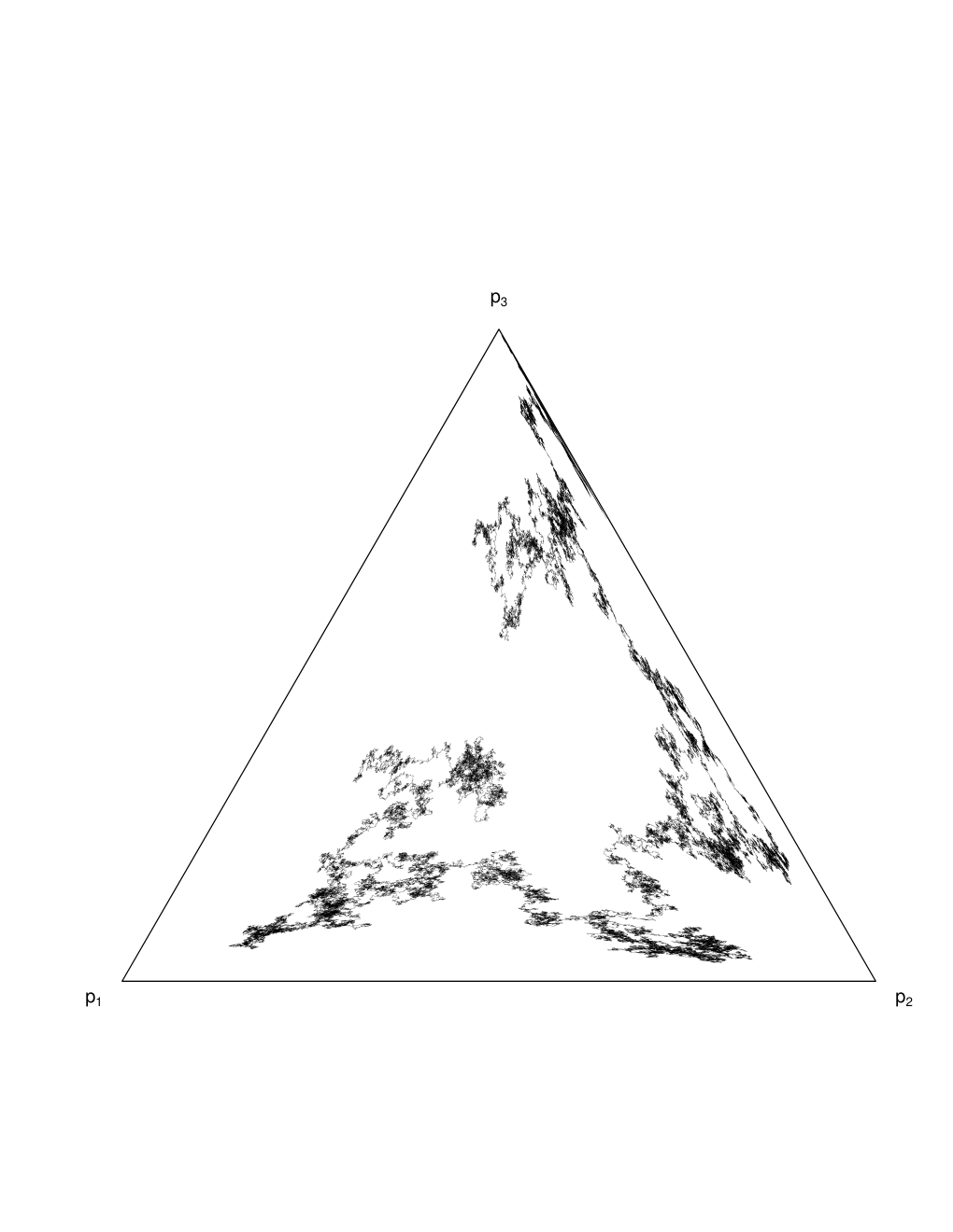
In the following we denote by $P_{t}^{X}$ the Markov semigroup associated to $X$, i.e. for bounded and measurable functions $f$ on $\Delta$ we set

$$P^{X}_{t}f(p):=\mathbb{E}\left[f(X_{t})|X_{0}=p\right].$$

(24)

Also, we write $P_{t}^{B}$ for the Brownian semigroup. The characterisations of the Aitchison diffusion which we discussed so far imply immediately the following properties of $P_{t}^{X}$.

Notice that $\lambda_{A}$ is not a finite measure on $\Delta$ in accordance with the fact that $X_{t}$ is transient, meaning $X_{t}\rightarrow\partial\Delta$ as $t\rightarrow\infty$ a.s. This again follows from the simple observation

$$\lim_{t\to\infty}\|X_{t}\|_{A}=\lim_{t\to\infty}\|B_{t}\|=\infty\ \text{a.s.}$$

In fact, one can even identify the distribution of the limit. Namely, first observe that

$$\lim_{t\to\infty}X_{t}=\lim_{t\to\infty}p\oplus\operatorname{sfm}(B_{t})\overset{d}{=}p\oplus\lim_{t\to\infty}\operatorname{sfm}(\sqrt{t}B_{1})=p\oplus\argmax(B_{1}).$$

Since that standard normal distribution attributes zero mass to the set of points in $\mathbb{R}^{n}$ which have no distinct maximum it follow that $\lim_{t\to\infty}X_{t}\sim\operatorname{Uniform}(\{\epsilon_{1},\dots,\epsilon_{n}\})$.

4. THREE APPROXIMATION RESULTS FOR THE AITCHISON DIFFUSION

In this section we want to provide three approximation results for the Aitchison diffusion, which rely on classical theorems from stochastic analysis or optimal transport and PDE theory, namely Wong-Zakai approximation, Donsker’s invariance principle and the JKO-scheme for the heat equation.

Recall, that in the introduction we alleged that the Aitchison diffusion, as described via the Stratonovich SDE

	$\displaystyle dX^{i}_{t}$	$\displaystyle=X^{i}_{t}\left(\circ dB^{i}_{t}-\sum_{j=1}^{n}X^{j}_{t}\circ dB^{j}_{t}\right),\quad i=1,\dots n$
	$\displaystyle X_{0}$	$\displaystyle=p\in\Delta,$

has the natural interpretation of being a replicator equation in a white noise fitness landscape. The first statement gives a justification for this assertion. Indeed, we will see that (3) can be derived from a replicator dynamic in a coloured noise fitness landscape, when sending the correlation length to zero.

To this end, consider on a probability space $(\Omega,\mathcal{F},\mathbb{P})$ the fitness landscape $y=(y_{t})_{t\geq 0}$, which is independent of the current population state, but evolves randomly and continuously in time as a Gaussian process with correlation structure

$$\mathbb{E}[y^{i}_{s}y^{j}_{t}]=\delta_{ij}e^{\lambda^{-2}|s-t|},\quad i,j=1,\dots n,$$

where $\lambda>0$ is a correlation length parameter. In other words, we assume that the fitness landscape $y$ is given by the $n$-dimensional Ornstein-Uhlenbeck process

$$\lambda^{2}dy_{t}=-y_{t}dt+\lambda dB_{t},$$

with $B$ an $n$-dimensional Brownian motion and $y_{0}\sim\mathcal{N}(0,\operatorname{Id}_{\mathbb{R}^{n}})$. Then we ascertain the following

Our second approximation result establishes a connection between random walks on the Aitchison simplex and (3) in the spirit of Donsker’s invariance principle [32, c.f.]. Therefore, first recall that the time discrete analogue of the replication dynamic (1) is given by the dynamical system

	$\displaystyle p_{i}^{(k+1)}$	$\displaystyle=\frac{p_{i}^{(k)}f^{i}\left(p^{(k)}\right)}{\sum_{j=1}^{n}p_{j}^{(k)}f^{j}\left(p^{(k)}\right)}$
	$\displaystyle p^{(0)}$	$\displaystyle=p\in\Delta.$

It was pointed out in [22] and [40] that we may think of this dynamic as modelling species adaptation by means of generation-wise Bayesian updating.

REFERENCES

- [1] http://www.compositionaldata.com/.
- [2] John Aitchison. The Statistical Analysis of Compositional Data. Journal of the Royal Statistical Society. Series B (Methodological), 44(2):139–177, 1982.
- [3] John Aitchison. The statistical analysis of geochemical compositions. Journal of the International Association for Mathematical Geology, 16(6):531–564, Aug 1984.
- [4] Luigi Ambrosio, Nicola Gigli, and Giuseppe Savaré. Gradient flows: in metric spaces and in the space of probability measures. Springer Science & Business Media, 2008.
- [5] N. Ay, J. Jost, H.V. Lê, and L. Schwachhöfer. Information Geometry. Ergebnisse der Mathematik und ihrer Grenzgebiete. 3. Folge / A Series of Modern Surveys in Mathematics. Springer International Publishing, 2017.
- [6] D. Bakry, I. Gentil, and M. Ledoux. Analysis and Geometry of Markov Diffusion Operators. Grundlehren der mathematischen Wissenschaften. Springer International Publishing, 2013.
- [7] Carles Barceló-Vidal, Josep Antoni Martín-Fernández, and Glòria Mateu-Figueras. Compositional Differential Calculus on the Simplex, chapter 13, pages 176–190. John Wiley & Sons, Ltd, 2011.
- [8] Dean Billheimer, Peter Guttorp, and William F. Fagan. Statistical Interpretation of Species Composition. Journal of the American Statistical Association, 96(456):1205–1214, 2001.
- [9] Vladimir I Bogachev, Nicolai V Krylov, Michael Röckner, and Stanislav V Shaposhnikov. Fokker-Planck-Kolmogorov Equations, volume 207. American Mathematical Soc., 2015.
- [10] François Bolley, Ivan Gentil, and Arnaud Guillin. Convergence to equilibrium in wasserstein distance for fokker–planck equations. Journal of Functional Analysis, 263(8):2430–2457, 2012.
- [11] G. Da Prato and J. Zabczyk. Ergodicity for Infinite Dimensional Systems. London Mathematical Society Lecture Note Series. Cambridge University Press, 1996.
- [12] Giuseppe Da Prato. An introduction to infinite-dimensional analysis. Springer Science & Business Media, 2006.
- [13] Manfred Eigen. Selforganization of matter and the evolution of biological macromolecules. Naturwissenschaften, 58(10):465–523, 1971.
- [14] Manfred Eigen and Peter Schuster. The hypercycle: a principle of natural self-organization. Springer Science & Business Media, 2012.
- [15] Ionas Erb and Nihat Ay. The information-geometric perspective of compositional data analysis, 2020.
- [16] Matthias Erbar. The heat equation on manifolds as a gradient flow in the Wasserstein space. Ann. Inst. H. Poincaré Probab. Statist., 46(1):1–23, 02 2010.
- [17] Wong Eugene and Zakai Moshe. On the relation between ordinary and stochastic differential equations. International Journal of Engineering Science, 3(2):213–229, 1965.
- [18] E Robert Fernholz. Stochastic portfolio theory. In Stochastic Portfolio Theory, pages 1–24. Springer, 2002.
- [19] Peter Friz and Martin Hairer. A course on rough paths. Preprint, 2014.
- [20] Drew Fudenberg and Christopher Harris. Evolutionary dynamics with aggregate shocks. Journal of Economic Theory, 57(2):420–441, 1992.
- [21] Bolin Gao and Lacra Pavel. On the Properties of the Softmax Function with Application in Game Theory and Reinforcement Learning. arXiv preprint arXiv:1704.00805, 2017.
- [22] Marc Harper. Information geometry and evolutionary game theory. arXiv preprint arXiv:0911.1383, 2009.
- [23] Josef Hofbauer, Lorens A Imhof, et al. Time averages, recurrence and transience in the stochastic replicator dynamics. The Annals of Applied Probability, 19(4):1347–1368, 2009.
- [24] Josef Hofbauer and Karl Sigmund. Evolutionary games and population dynamics. Cambridge university press, 1998.
- [25] Julian Hofrichter, Jürgen Jost, and Tat Dat Tran. Information geometry and population genetics. Springer, 2017.
- [26] Nobuyuki Ikeda and Shinzo Watanabe. Stochastic differential equations and diffusion processes, volume 24. Elsevier, 2014.
- [27] Lorens A Imhof. The long-run behavior of the stochastic replicator dynamics. The Annals of Applied Probability, 15(1B):1019–1045, 2005.
- [28] Richard Jordan, David Kinderlehrer, and Felix Otto. The variational formulation of the Fokker–Planck equation. SIAM journal on mathematical analysis, 29(1):1–17, 1998.
- [29] Nathan Krislock and Henry Wolkowicz. Euclidean distance matrices and applications. In Handbook on semidefinite, conic and polynomial optimization, pages 879–914. Springer, 2012.
- [30] Terry J Lyons, Michael Caruana, and Thierry Lévy. Differential equations driven by rough paths. Springer, 2007.
- [31] Luca Natile, Mark A Peletier, and Giuseppe Savaré. Contraction of general transportation costs along solutions to Fokker–Planck equations with monotone drifts. Journal de mathématiques pures et appliquées, 95(1):18–35, 2011.
- [32] Charles M Newman, A Larry Wright, et al. An invariance principle for certain dependent sequences. The Annals of Probability, 9(4):671–675, 1981.
- [33] Martin A. Nowak. Evolutionary dynamics. Harvard University Press, 2006.
- [34] Felix Otto. The geometry of dissipative evolution equations: The porous medium equation. Communications in Partial Differential Equations, 26(1-2):101–174, 2001.
- [35] Grigorios A. Pavliotis. Stochastic processes and applications: diffusion processes, the Fokker-Planck and Langevin equations, volume 60. Springer, 2014.
- [36] Vera Pawlowsky-Glahn, Juan José Egozcue, and Raimon Tolosana Delgado. Lecture notes on compositional data analysis. 2007.
- [37] Vera Pawlowsky-Glahn et al. Statistical modeling on coordinates, 2003.
- [38] Ross G. Pinsky. Positive Harmonic Functions and Diffusion. Cambridge Studies in Advanced Mathematics. Cambridge University Press, 1995.
- [39] Siavash Shahshahani. A new mathematical framework for the study of linkage and selection. American Mathematical Soc., 1979.
- [40] Cosma Rohilla Shalizi et al. Dynamics of bayesian updating with dependent data and misspecified models. Electronic Journal of Statistics, 3:1039–1074, 2009.
- [41] Karl Sigmund. A survey of replicator equations. In Complexity, Language, and Life: Mathematical Approaches, pages 88–104. Springer, 1986.
- [42] J Maynard Smith and George R Price. The logic of animal conflict. Nature, 246(5427):15, 1973.
- [43] D.W. Stroock and K. Itō. Markov Processes from K. Itô’s Perspective. Academic Search Complete. Princeton University Press, 2003.
- [44] Peter D Taylor and Leo B Jonker. Evolutionary stable strategies and game dynamics. Mathematical biosciences, 40(1-2):145–156, 1978.
- [45] K.G. van den Boogaart and R. Tolosana-Delgado. Analyzing Compositional Data with R. Use R! Springer Berlin Heidelberg, 2013.
- [46] Max-K von Renesse and Karl-Theodor Sturm. Transport inequalities, gradient estimates, entropy and ricci curvature. Communications on pure and applied mathematics, 58(7):923–940, 2005.
- [47] E. Dokumaci W. H. Sandholm and F. Franchetti. Dynamo: Diagrams for evolutionary game dynamics., 2012.
- [48] Bin Wu, Chaitanya S Gokhale, Matthijs van Veelen, Long Wang, and Arne Traulsen. Interpretations arising from Wrightian and Malthusian fitness under strong frequency dependent selection. Ecology and evolution, 3(5):1276–1280, 2013.