Vectorized Hankel Lift: A Convex Approach for Blind Super-Resolution of Point Sources 00footnotetext: Authors are listed alphabetically.
Abstract
We consider the problem of resolving point sources from samples at the low end of the spectrum when point spread functions (PSFs) are not known. Assuming that the spectrum samples of the PSFs lie in low dimensional subspace (let denote the dimension), this problem can be reformulated as a matrix recovery problem, followed by location estimation. By exploiting the low rank structure of the vectorized Hankel matrix associated with the target matrix, a convex approach called Vectorized Hankel Lift is proposed for the matrix recovery.
It is shown that samples are sufficient for Vectorized Hankel Lift to achieve the exact recovery. For the location retrieval from the matrix, applying the single snapshot MUSIC method within the vectorized Hankel lift framework corresponds to the spatial smoothing technique proposed to improve the performance of the MMV MUSIC for the direction-of-arrival (DOA) estimation.
Keywords. blind super-resolution, vectorized Hankel lift, low rank, MUSIC
1 Introduction
1.1 Problem formulation
In this paper, we study the super-resolution of point sources when point spread functions (PSFs) are not known. More specifically, consider a point source signal of the form
| (1.1) |
where is the Dirac function, and are the locations and amplitudes of the point source signal, respectively. Let be its convolution with unknown point spread functions,
| (1.2) |
where are the point spread functions depending on the locations of the point sources.
Taking the Fourier transform on both sides of (1.2) yields
| (1.3) |
The goal in blind super-resolution is to recover from the low end of the spectrum
| (1.4) |
when , , are not known. Here we assume the index rather than only for convenience of notation. In addition to blind super-resolution, the observation model (1.4) also arises from many other important applications, such as 3D single-molecule microscopy [47], multi-user communication system [43] and nuclear magnetic resonance spectroscopy [46].
It is evident that the blind super-resolution problem is ill-posed without any further assumptions. To address this issue, we assume that the set of vectors corresponding to the unknown point spread functions belong to a common and known low-dimensional subspace represented by , i.e.,
| (1.5) |
where is the unknown orientation of in this subspace. As is pointed out in [60], the subspace assumption is reasonable in several application scenarios. Moreover, it has been extensively used in the literature, see for example [1, 18, 60, 33, 37].
For any , define the vector as
| (1.6) |
Let be the th column vector of . If we define the matrix as
| (1.7) |
then under the subspace assumption (1.5) and using the lifting trick [1, 12, 19, 18, 60, 38, 64, 42, 37], the observation model (1.4) can be reformulated as a linear measurement of :
| (1.8) |
where the inner product of two matrices is given by , is th column of the identity matrix , and throughout this paper vectors and matrices are indexed starting with zero. Moreover, we can further rewrite (1.8) in the following compact form,
| (1.9) |
where is a linear operator defined by . The adjoint of the operator , denoted , is defined as .
Based on the above reformulation of blind super-resolution under the subspace assumption, it can be seen that the key is to recover from the linear measurement vector . Once is reconstructed, the frequency components can be extracted from by the subspace methods which will be detailed in Section 2.2. After the frequency components are obtained, can be recovered by solving a least squares system. Moreover, due to the multiplicative form of and in (1.7), we only expect to recover them separately up to a scaling ambiguity. Thus, we will assume that without loss of generality.
Note that the formulations in (1.4) and (1.9) are by no means new and they have been utilized in [60]. Moreover, when the point spread function is shared among all point sources (i.e., the stationary case), (1.4) reduces to the blind sparse spikes deconvolution model considered in [18]. To recover the target matrix from the linear measurements , following the approach developed in [53] for spectrally sparse signal recovery, a similar atomic norm minimization method is proposed in [60],
| (1.10) |
where the atomic norm is defined as
The successful recovery guarantee of (1.10) is studied in [60], while the robust analysis is provided separately in [33]. Note that for spectrally sparse signal recovery, in addition to atomic norm minimization, there are also methods which exploit the low rank property of the structured matrix formed from the signal [15, 6, 7]. This motivates us to develop a low rank approach for blind super-resolution.
1.2 Exploiting the low rank structure: Vectorized Hankel Lift
We start with a brief view of spectrally sparse signal recovery based on the hidden low rank structure. Let be a spectrally sparse signal consisting of complex sinusoids,
Let be a vector of length which is obtained by sampling at contiguous, equally-spaced points. In a nutshell, spectrally sparse signal recovery is about reconstructing the signal from its partial samples. Recalling the definition of in (1.6), we can represent as
| (1.11) |
Let be a linear operator which maps a vector into an Hankel matrix,
| (1.12) |
where is the th entry of and . Without loss of generality, we assume in this paper. Due to the particular expression of in (1.11), it is not hard to see that the rank of is at most according to the Vandermonde decomposition of [15].
Note that the expression for the data matrix in (1.7) is overall similar to that for the spectrally sparse vector in (1.11), except that the weights in front of in (1.7) are vectors and consequently is a matrix rather than a vector. Intuitively, if we treat each column of as a single element and form a matrix in the same fashion as in (1.12), it can be expected that the resulting matrix is also low rank. This is indeed true. Specifically, let be the vectorized Hankel lifting operator which maps a matrix with columns into an matrix,
| (1.13) |
where . To distinguish the matrix in (1.13) from the one in (1.12), we refer to as the vectorized Hankel matrix associated with . Then a simple algebra yields that the vectorized Hankel matrix associated with appearing in the blind super-resolution problem admits the following decomposition:
| (1.14) |
where the matrices and are given by
| (1.15) |
and
| (1.16) |
It follows immediately that the rank of is at most and thus it is a low rank matrix when is smaller than .
In this paper we adopt the popular nuclear norm minimization to exploit the low rank structure of , yielding a convex approach for the reconstruction of which is also referred to Vectorized Hankel Lift. Exact recovery guarantee will be established based on certain assumptions on the subspace matrix in (1.5).
1.3 Other Related Work
In this section, we give a brief introduction of other related work in addition to [18, 60, 33]. When the point spread functions are known and do not depend on the locations of the point sources, the measurement model (1.4) reduces to
| (1.17) |
In this case, estimating the locations and amplitudes from is typically known as super-resolution or line spectrum estimation. This problem arises in many areas of science and engineering, such as array imaging [31, 52], Direction-of-Arrival (DOA) estimation [51], and inverse scattering [26]. The solution to this problem can date back to Prony [45]. In the Prony’s method, the locations are retrieved from the roots of a polynomial whose coefficients form an annihilating filter for the observation vector. Nevertheless, the Prony’s method is numerical unstable despite that in the noiseless setting successful retrieval is guaranteed in exact arithmetic. As alternatives, several subspace methods have been developed, including MUSIC [50], ESPRIT [48], and the matrix pencil method [29]. In the absence of noise, the subspace methods are also able to identify the locations of the point sources. When there is noise, the stability of these methods has been studied in [41, 40, 35, 44] in the regime when , where is the minimum (wraparound) separation between any two locations, and is a proper numerical constant. The analysis essentially relies on the lower bound on the smallest singular value of the Vandermonde matrix. The super-resolution limits of MUSIC and ESPRIT have been discussed in [34, 35], which is about the noise level that can be tolerated in order for the algorithms to achieve super-resolution when . In this regime, it is difficult to obtain a general and nontrivial lower bound on the smallest singular value of the Vandermonde matrix. Thus, the super-resolution limits in [34, 35] are established for point sources whose locations obey certain configurations.
Inspired by compressed sensing and low rank matrix reconstruction, various optimization based methods have also been developed for super-resolution and related problems. In [9], the total variation (TV) minimization method is used to resolve the locations of the point sources. It is shown that when , exact recovery of the locations can be guaranteed. Moreover, the solution to the TV minimization problem can be computed by solving a semidefinite programming (SDP). Note, in the discrete setting, super-resolution can be interpreted within the framework of compressed sensing. However, since the measurement model in super-resolution considers the low end spectrum, and hence is deterministic, the typical successful recovery guarantee for compressed sensing [11] cannot sufficiently explain the success of the TV norm minimization method for super-resolution. The robustness of TV norm minimization is studied in [8], and the super-resolution problem of non-negative point sources is considered in [22, 49, 20, 21, 23]. Moreover, super-resolution from time domain samples has been investigated in [2, 4, 23].
When only partial entries of are observed in (1.17), filling in the missing entries is indeed the spectrally sparse signal recovery problem. Motivated by the work in [13], an atomic norm minimization method (ANM) is proposed for this problem. It is shown that can be reconstructed from random samples provided the frequencies are well separated. ANM has been extended in [39, 63] to handle the case when multiple measurement vector (MMV) are available. In the setting of MMV, multiple snapshots of observations are collected and they share the same frequencies information. As already mentioned previously, the Hankel matrix corresponding to is a low rank matrix. Consequently, spectrally sparse signal recovery can be reformulated as a low rank Hankel matrix completion problem, and replacing the rank objective with the nuclear norm yields a recovery method known as EMaC. It has been shown that EMaC is able to reconstruct a spectrally sparse signal with high probability provided the number of observed entries is . In [61], a formulation of EMaC for the multi-snapshots scenario is presented. Additionally, based on the low rank property of the Hankel matrix, provable non-convex algorithms have been developed in [6, 7] to reconstruct spectrally sparse signals. Later, Zhang et.al. [65] extend one of the non-convex algorithms to complete an MMV matrix, and in this work the same vectorized Hankel lift technique is used to exploit the hidden low rank structure. Recently, a matrix completion problem based on the low dimensional structure in the transform domain is studied in [14]. More precisely, it is assumed that after applying the Fourier transform to each column of the target matrix, each row of the resulting matrix will be a spectrally sparse signal. Since it does not require the spectrally signals share the same frequency information, a block-diagonal low rank structure is adopted to exploit the low dimensional structure. Exact recovery guarantee is also established provided the sampling complexity is nearly optimal.
Apart from super-resolution and spectrally sparse signal recovery, our work is also related to blind deconvolution. After the reparametrization of the signal and blurring kernel under the subspace assumption [1], the goal in blind deconvolution is to recover the vectors and simultaneously from the measurement vector in the form of
Noting that the above measurement model can be reformulated as a linear operation on a rank- matrix, a nuclear norm minimization method is proposed for blind deconvolution. The performance guarantee of the method has been established in the case when is a partial Fourier matrix and is a Gaussian matrix. A non-convex gradient descent approach for blind deconvolution is developed and analyzed in [37], and the identifiability problem is studied in [38, 19].
1.4 Notation and Organization
Throughout this work, vectors, matrices and operators are denoted by bold lowercase letters, bold uppercase letters and calligraphic letters, respectively. Note that vectors and matrices are indexed starting with zero. The letter denotes the identity operator. We use to denote the matrix defined by
| (1.18) |
where is a constant defined as
| (1.19) |
In fact, forms an orthonormal basis of the space of Hankel matrices.
We use to denote the th entry of and or to denote the th entry of . Additionally, the th row and th column of are denoted by and , respectively. Furthermore, we use the MATLAB notation to denote a vector of size , with entries , i.e.,
For any matrix , and are used to denote the trace, conjugate transpose, transpose and column vectorization of , respectively. Also, , and denote its spectral norm, Frobenius norm and nuclear norm, respectively.
We use to denote the diagonal matrix specified by the vector . For a natural number , we use to denote the set . For any two matrices of the same size, their inner product is defined as . Moreover, we will refer to as the Hadamard, Kronecker product and Khatri-Rao product respectively. More precisely, the Hadamard product is the element-wise product of two matrices and the Kronecker product between and is given by
and the Khatri-Rao product is given by
where , denote the th column of and , respectively. By the application of the Khatri-Rao product, we can rewrite in (1.15) as , where and are matrices given by
| (1.20) |
and .
Throughout this paper, denote absolute positive numerical constants whose values may vary from line to line. The notation means that there exists an absolute constant such that . Similarly, the notation means that there exists an absolute constant such that .
The rest of this paper is organized as follows. Section 2 begins with the presentation of Vectorized Hankel Lift and its recovery guarantee, followed by the retrieval of the point source locations. Numerical results to demonstrate the performance of Vectorized Hankel Lift is presented at the end of Section 2. The proofs of the main result are provided from Section 3 to Section 6. Finally, we conclude this paper with a few future directions in Section 7.
2 Vectorized Hankel Lift and Frequency Retrieval
2.1 Vectorized Hankel Lift and recovery guarantee
Under the assumption that is a low rank matrix, it is natural to reconstruct by solving the affine rank minimization problem
| (2.1) |
However, the problem (2.1) is computational intractable due to the rank objective. Since the nuclear norm of a matrix is the tightest convex envelope of the matrix rank, seeking a solution with a small nuclear norm is also able to enforce the low rank structure. Therefore, instead of solving (2.1) directly, we consider the following nuclear norm minimization problem for the recovery of :
| (2.2) |
In this paper, we refer to (2.2) as Vectorized Hankel Lift. There are many existing software packages that can be used to solve this problem. Thus we restrict our attention on the theoretical recovery guarantee of Vectorized Hankel Lift and investigate when the solution of (2.2) coincides with .
We need to reformulate (2.2) in order to facilitate the analysis. Let be an matrix which can be expressed as
where for and . Recall that is the vectorized Hankel lift operator defined in (1.13). The adjoint of , denoted , is a linear mapping from matrices to matrices of size . In particular, for any matrix , the th column of is given by
Letting , we have
where the scalar is defined as
Moreover, we define . Then
| (2.3) |
where the set of matrices defined in (1.18) forms an orthonormal basis of the space of Hankel matrices. The adjoint of , denoted , is given by . Additionally, and satisfy
Letting , it can be readily verified that
Furthermore, define . We have for any matrix . Therefore, the optimization problem (2.2) can be reformulated as
| (2.4) |
Due to the equivalence between (2.2) and (2.4), it suffices to investigate the recovery guarantee of (2.4). To this end, we make two assumptions.
Assumption 2.1.
The column vectors of the subspace matrix are independently and identically sampled from a distribution which obeys the following properties:
- •
Isotropy property. A distribution obeys the isotropy property if for ,
(2.5) - •
Incoherence property. A distribution satisfies the incoherence property with parameter if for ,
(2.6) holds, where denotes the th entry of .
- •
For , the sampled column vectors satisfy
(2.7)
The first two conditions (2.5) and (2.6) in Assumption 2.1 are first introduced in [10] in the context of compressed sensing and these two properties are also made in [18, 60, 33] for the blind super-resolution problem. If has mean zero, the isotropy condition states that the entries of have unit variance and are uncorrelated, which implies in the incoherence property. The lower bound is achievable by several examples, for instance, when the components of are Rademacher random variables taking the values with equal probability or is uniformly sampled from the rows of a Discrete Fourier Transform (DFT) matrix. In addition to (2.5) and (2.6), we also need (2.7) to establish our main result. However, we would like to point out that (2.7) is not a stringent condition, but holds (either trivially or with high probability) by many common random ensembles.
- •
If the components of are Rademacher random variables or is uniformly sampled from the rows of a DFT matrix, it is trivial that for any fixed , .
- •
Assumption 2.2.
Assumption 2.2 is the same as the one made in [15, 6, 7] for spectrally sparse signal recovery. Later, we will show that also holds when , see Lemma 3.3. Recalling the definition of and , this assumption is essentially about the conditioning property of the Vandermonde matrix. This property is studied in [41] through the discrete Ingham inequality [30] and in [44] through the discrete large sieve inequality [56]. In particular, it follows from [44] that Assumption 2.2 holds when the minimum wrap-around distance between the frequencies, denoted , satisfies
| (2.9) |
We are in position to present the main result of this paper.
Theorem 2.1 (Exact recovery guarantee of Vectorized Hankel Lift).
Remark 2.1.
The sampling complexity established in [60] for the atomic norm minimization method is . While this is slightly better than the sampling complexity for Vectorized Hankel Lift, our analysis is based on less stringent assumptions. In our analysis, the coefficients are not required to be i.i.d. samples from the uniform distribution on the complex unit sphere, but can be any unit norm vectors. In addition, noting that the right-hand side of (2.9) is about for moderately large , which is smaller than , the separation required in the main result of [60]. It is worth noting that the robust analysis of the atomic norm minimization method has been studied in [33] and we will leave the robust analysis of Vectorized Hankel Lift for future work.
The proof of Theorem 2.1 follows a well established route that has been widely used for compressed sensing and low rank matrix recovery. In a nutshell, a dual variable needs to be constructed to verify the optimality of . That being said, the details of the proof itself are nevertheless quite involved and technical, and cannot be covered by the results from existing works. In particular, we need to show that there exists a partition of the measurements satisfying a list of desirable properties in order to construct the dual certificate.
2.2 Variants of MUSIC for frequency retrieval
In this section, we discuss the subspace method, particularly the MUltiple SIgnal Classification (MUSIC) algorithm [50], for computing the frequency parameters from the matrix . Note that once are obtained, the weights can be computed by solving an overdetermined linear system. As can be seen later, applying the idea of the single snapshot MUSIC to yields a variant which is equivalent to the existing spatial smoothing technique proposed to improve the performance of the Multiple Measurement Vector (MMV) MUSIC.
The careful reader may notice that every single row of is a spectrally sparse signal of the form (1.11), and moreover, all the rows share the same frequency parameters . Thus we can apply the single snapshot MUSIC algorithm to a row of for frequency retrieval. Let . Recall that is the Hankel matrix of rank and it admits the Vandermonde decomposition
| (2.10) |
Moreover, letting
| (2.11) |
be the SVD of , where and , it is evident that and span the same column space. Note that , where . It follows from the property of the Vandermonde matrix that
if and only if .
Therefore we conclude that if and only if . The single snapshot MUSIC algorithm utilizes this idea to identify the frequencies, and it consists of the following two steps:
- 1.
Compute the SVD of as in (2.11);
- 2.
Identify as the largest local maxima of the pseudospectrum: .
Here we present the single snapshot MUSIC algorithm directly based on the Hankel matrix . Equivalently, it can be interpreted from the autocorrelation matrix model for signals, see for example [32] and references therein. In the noiseless setting, it is easy to see that the single snapshot MUSIC algorithm is able to compute exactly. When noise exists in , the procedure of the algorithm remains unchanged, but with the SVD of being replaced by the SVD of the noisy Hankel matrix and with being the left singular vectors corresponding to the smallest singular values. The stability analysis of the single snapshot algorithm is discussed in [41].
To motivate the new variant of the MUSIC algorithm for estimating the frequencies from , we note that appears as a separate component both in the Vandermonde decomposition of and that of , see (1.14) and (2.10). Therefore, we can replace the SVD of with the SVD of in the first step of the single snapshot MUSIC algorithm. This gives the following variant:
- 1.
Compute the SVD of : , where and ;
- 2.
Identify as the largest local maxima of the pseudospectrum: .
The following lemma establishes a connection between this variant and the single snapshot MUSIC, showing that the former one actually utilizes the SVD of the matrix formed by stacking all () together.
Lemma 2.2.
Let be a matrix constructed by stacking all on top of one another:
There exists a permutation matrix such that .
Proof.
Following the Vandermonde decomposition, the th block of can be rewritten as
where is the th column of and is the th entry of . Thus has the following decomposition
According to the commutative law in [66, Section 1.10.3], there exists a permutation matrix such that . ∎
Based on Lemma 2.2, we will see that the variant obtained by applying the single snapshot MUSIC idea to corresponds to the spatial smoothing technique (more precisely the forward only spatial smoothing technique). First, treating the rows of as i.i.d samples of a random signal whose covariance matrix can be used to compute the signal space as in (2.11), MMV MUSIC [52] uses the principal eigenspace of the empirical covariance matrix (up to a scaling factor )
to compute . However, when the signal comes from coherence sources, the performance of MMV MUSIC will degrade. To deal with this difficulty, the forward only spatial smooth technique proposes to increase the number of samples by partitioning each into overlapped short samples (with each short sample being of length , where ), and then construct the empirical covariance matrix from all the short samples. A simple algebra yields that the new empirical covariance matrix is indeed given by (up to a scaling factor )
It is not hard to see that the principal eigenspace of is the same as the principal singular vector space of . Thus, by Lemma 2.2, we know that the variant obtained by applying the single snapshot MUSIC idea to is equivalent to the spatial smoothing MUSIC. For more details about spatial smoothing, see [25, 24, 62].
2.3 Extension to higher dimension
Vectorized Hankel Lift and the analysis are easily extended to higher dimensional array recovery problem. For ease of exposition, we give a brief discussion of the two-dimensional (2D) case but emphasize that the situation in higher dimensions is similar. For the 2D blind super-resolution problem, the data matrix can be expressed as
where is the amplitude, is the 2D frequency and corresponds to the Fourier samples of the unknown 2D point spread function. Letting for , the 2D data array can be rewritten in a more compact form:
Likewise, we assume that there exists a subspace matrix such that for any . Then
For any , the th entry of is given by
where is the th column of . Therefore, we have , where , and is a linear operator given by
As in the 1D case, the blind super-resolution problem is essentially about recovering the target matrix from the observation vector .
Note that the target matrix can be rewritten as the following block form:
Letting , we define the two-fold vectorized Hankel lift of as follows:
where is the vectorized Hankel matrix defined in (1.13). It can be readily shown that has the following decomposition
| (2.12) |
where are two matrices defined in (1.20) and (1.16) but with the frequencies , and .
If all frequencies are distinct and all are non-zeros, it is not hard to see that is a low rank matrix. Therefore, we can recover by solving the following convex programming
| (2.13) |
The recovery guarantee of (2.13) can be similarly established in the following theorem. The proof details are overall similar to that for Theorem 2.1, and thus are omitted.
Theorem 2.3.
Under Assumption II.1 and suppose and , the data matrix is the unique optimal solution to (2.13) with probability at least for absolute constants , provided that .
2.4 Numerical Experiments
In this section, we empirically evaluate the performance of Vectorized Hankel Lift for the recovery of in the blind super-resolution problem. Vectorized Hankel Lift is solved by SDPT3 [54] based on CVX [27]. The recovery ability of Vectorized Hankel Lift will be evaluated via the framework of empirical phase transition and we compare it with the atomic norm minimization method [60]. The locations of the point source signals are generated randomly from , while the amplitudes are generated via with being uniformly sampled from and being uniformly sampled from . The subspace matrix are sampled from two random ensembles which all satisfy the conditions in Assumption 2.1. The first one is the random submatrix sampled from the DFT matrix, and the other one is the random matrix whose entries satisfy the uniform distribution over . The coefficients are i.i.d. standard Gaussian random vectors followed by normalization. In our tests, 20 Monte Carlo trails are repeated for each problem instance and we report the probability of successful recovery out of those trials. A trail is declared to be successful if the relative reconstruction error of in terms of the Frobenius norm is less than .
We first fix and vary the values of and . Figure 1(a) and Figure 1(b) show the phase transitions of Vectorized Hankel Lift and atomic norm minimization method when the subspace matrix is randomly sampled from the DFT matrix and the locations of point sources are randomly generated without imposing the separation condition, and Figure 1(c) illustrates the phase transition of the atomic minimization method when the separation condition is imposed. Here we omit the phase transition plot of Vectorized Hankel Lift for the frequency separation case because the plot is similar to Figure 1(a). It can be observed that the atomic norm minimization method has a higher phase transition curve when the separation condition is satisfied. However, in contrast to Vectorized Hankel Lift, its performance degrades severely when there is no frequency separation requirement. That is, Vectorized Hankel Lift is less sensitive to the separation condition. We also conduct the phase transition tests when the entries of are i.i.d. sampled from the uniform distribution over . The phase transition diagrams are presented in Figure 2, and similar observations can be made. Note that the phase transition plot of Vectorized Hankel Lift for the frequency separation case is still omitted due to the high similarity with Figure 2(a).


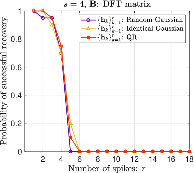
In the above phase transition tests, the coefficients are sampled from random Gaussian with normalization. In order to test whether the choice of matters, we also test another two cases for the coefficients. One is the Identical Gaussian, where are the same across (sampled from random Gaussian with normalization). The other one is QR where are obtained from the Q matrix in the QR decomposition of an random Gaussian matrix. Tests are conducted for fixed and , and the plots of successful recovery probability against the number of spikes are presented in Figure 3. It can be clearly seen that no significant differences over different types of are observed from the plots. Therefore, the numerical results validate that our main result can hold without any conditions of .

In order to examine the effect of the separation condition more carefully, we further conduct tests for fixed , , and vary the number of samples . In the tests, we impose that there are at least two spikes with separation equal to and , respectively. For each problem instance, we repeat 50 Monte Carlo trails and report the probability of successful recovery out of those trials. The numerical results are presented in Figure 4. It is evident that Vectorized Hankel Lift presents a better performance when the minimum separation is . When the spikes are well separated (i.e., the minimum separation is ), the atomic norm minimization method performs better. In addition, the results confirm that Vectorized Hankel Lift is overall not affected by the separation condition.


We also plot the locations of the point sources and the unknown point spread function samples computed from for a random instance corresponding to and . We apply the MUSIC variant introduced in Section 2.2 (i.e., the spatial smoothing MUSIC) to localize the . Figure 5(a) shows the pseudospectrum on a set of points on with equal distance . As can be seen from this figure, the function peaks at the locations of true frequencies. After the are identified, the coefficients are computed by solving a least squares problem and are estimated as . Figure 5(b) includes the plots of the estimates of against the true values which clearly show that can be recovered.


3 Proof Architecture of Main Result
3.1 Preliminaries
We first apply the bounded difference inequality to show that for the column vectors with independent entries, the condition (2.7) in Assumption 2.1 holds with high probability given (2.5) and (2.6).
Lemma 3.1.
Proof.
Next, we present a lemma about the basic properties of the linear operator .
Lemma 3.2.
Proof.
The properties in (3.3) follows directly from the definition of . For the left inequality, we have
The right one can be proved as follows
The proof is now complete. ∎
The following lemma suggests that the smallest singular value of can be lower bounded by the smallest singular value of .
Lemma 3.3.
Proof.
Let be the th column of . Since , it can be easily seen that
Recall that a selection matrix is the unique matrix such that
and it has the remarkable property that [57, Corollary 2]. Thus we have
which completes the proof. ∎
A straightforward application of Lemma 3.3 yields the following result, which can be regarded as a variant of [7, Lemma 1].
Lemma 3.4.
Suppose obeys the incoherence condition (2.8) with parameter . Let be the singular value decomposition of , where and . If we rewrite as
where the th block is for , then
| (3.4) |
Proof.
The following corollary is a direct consequence of Lemma 3.4 and will be frequently used in the sequel.
Corollary 3.5.
Suppose obeys the incoherence condition (2.8) with parameter . Then,
| (3.5) |
The matrix Bernstein inequality, stated below, will be used frequently in our analysis.
3.2 Deterministic optimality condition
As is typical in the analysis of low rank matrix recovery, in order to show that is the unique optimal solution to the convex program (2.4), we need to construct a dual certificate which satisfies a set of sufficient conditions. These conditions can be viewed as a variant of the KKT condition for the optimality of . Recall that the singular value decomposition (SVD) of is . The tangent space of the nuclear norm at can be defined as
The projections onto the tangent space can be defined as
| (3.7) |
and the corresponding projector onto the orthogonal complement of is given by .
Theorem 3.7.
Suppose and
| (3.8) |
If there exists a dual certificate such that
| (3.9) | ||||
| (3.10) | ||||
| (3.11) |
then is the unique solution to (2.4).
Proof.
The structure of the proof is overall similar to those in [15, 16, 14]. Consider any feasible solution , where the perturbation satisfies
| (3.12) | ||||
| (3.13) |
The first condition (3.12) implies that is in the null space of , while the second condition (3.13) guarantees that has the vectorized Hankel structure. Note that for any matrix , there exists an matrix such that
In the meantime, we have . Thus,
| (3.14) |
The condition (3.11) directly implies that there exists a vector such that
Therefore, combining (3.11) and (3.13), we obtain
Moreover, the second term of (3.14) can be upper bounded as follows:
where the last step is due to (3.9) and (3.10). Consequently,
where the fourth line is due to Lemma 6.1 in Section 6. It follows that unless .
Note that requires , which in turn requires . In this case, we have
which implies that . Thus is the unique minimizer. ∎
3.3 Constructing the dual certificate
It is intuitively clear that we may construct a dual certificate obeying the conditions (3.9), (3.10) and (3.11) by solving the following constrained least squares problem:
Here only the conditions (3.9) and (3.11) are taken into account because once is small, the projection of onto can be simultaneously small.
Applying the projected gradient method to solve the above optimization problem, we obtain the following update rule:
However, due to the statistical dependence among the iterations, the convergence analysis of the vanilla gradient iteration is difficult. Therefore, the golfing scheme [28] proposes to break the statistical independence by dividing all the linear measurements into a few disjoint partitions and use a fresh partition in each iteration.
Assume we divide the linear measurements in (1.8) into partitions, denoted , and let . Define
| (3.15) |
and
| (3.16) |
Then the golfing scheme for the construction of satisfying the conditions in Theorem 3.7 can be formally expressed as
| (3.17) | ||||
Evidently the property of relies on the partitions . In order to construct the desirable , we require to satisfy a set of conditions list in the following lemma, in which we have
| (3.18) |
The proof of this lemma will be presented in Section 4.
Lemma 3.8.
Let and set . If , then there exists a partition such that the following properties hold :
| (3.19) | ||||
| (3.20) | ||||
| (3.21) | ||||
| (3.22) | ||||
| (3.23) |
Here is fixed. Recalling the definition of the operator in (3.16) , the expectation is taken with respect to .
3.4 Validating the dual certificate and completing the proof
In this section we show that the dual certificate constructed from the iteration (3.17) satisfies the conditions in Theorem 3.7. The result follows from several lemmas that will be proved in Section 5. In these lemmas, is a partition of satisfying the conditions in Lemma 3.8, and are the associated linear operators defined in (3.15). Note that we assume (3.4) holds in the remainder of this paper, which follows from Assumption 2.2 and Lemma 3.4.
Lemma 3.9.
Assume . Under the condition (III.18) of Lemma 3.8, the event
| (3.24) |
occurs with probability at least for a universal constant .
The following corollary is the special case of Lemma 3.9 when and .
Corollary 3.10.
Assume . The event
| (3.25) |
occurs with probability at least for a universal constant .
Lemma 3.11.
Under the condition (III.19) of Lemma 3.8, for any and fixed , the event
| (3.26) |
occurs with probability at least for a universal constant .
Lemma 3.12.
Under the condition (III.20) of Lemma 3.8, for any and fixed , the event
| (3.27) |
occurs with probability at least for a universal constant .
Lemma 3.13.
Under the condition (III.21) of Lemma 3.8, for any and fixed , the event
| (3.28) |
occurs with probability at least for a numerical constant .
Lemma 3.14.
Recalling that and satisfy (3.4), we have
| (3.29) |
Equipped with these lemmas, we are in position to validate the conditions in Theorem 3.7. Note that holds due to (3.2) in Lemma 3.2, and (3.8) is proved in Corollary 3.10. As for (3.11), it follows immediately from the construction of . Thus, it remains to validate (3.9) and (3.10).
Validating (3.9)
Validating (3.10)
First recall that . According to (3.17), we have
Then it follows that
| (3.31) |
where the second line follows from the fact that .
For any , Lemma 3.11 implies that
| (3.32) |
Recalling from the equality (3.30), we have
Applying Lemma 3.12 and Lemma 3.13 yields that
| (3.33) |
and
| (3.34) |
After substituting (3.33) and (3.34) into (3.32), we have
where step holds provided .
Finally, noting that , the application of Lemma 3.14 gives
when , where the first inequality follows from (3.31).
Thus we have shown that the dual certificate constructed from the iteration (3.17) satisfies the conditions in Theorem 3.7 with probability at least provided that . Corollary 3.10 implies (3.8) holds with probability at least if . Taking an upper bound on the number of measurements completes the proof of Theorem 2.1.
4 Proof of Lemma 3.8
In this section, we will use probabilistic argument to show that the events (3.19) - (3.23) occur with high probability if we construct in a random manner and thus conclude that there at least exists a partition satisfying (3.19) - (3.23).
Let be independent random variables, each of which takes value in uniformly at random. For any , we construct as follows:
Clearly, form a partition of . For any fixed , we also have
Therefore can be viewed as the sum of Bernoulli random variables, i.e.,
| (4.1) |
where are i.i.d. Bernoulli random variables with parameter . The application of the Hoeffding inequality yields that holds with probability at least for a universal constant . Then we can take the uniform bound to obtain
where the last inequality is due to .
Our next goal is to show that the events (3.20) - (3.23) occur with high probability. We will first apply the matrix Bernstein inequality (3.6) to obtain the desired upper bounds for fixed , and then take the uniform bound analysis to complete the proof.
4.1 Proof of (3.20)
For any , by the definition of in (3.16), we have
where the third line follows from the isotropy property (2.5) of .
As a result, one has the following equality
where is the Bernoulli random variable defined in (4.1) and is the operator defined as
for any . It is easy to verify that is self-adjoint and positive semi-definite.
In order to apply the matrix Bernstein inequality (3.6) to bound , one needs to bound and .
For the upper bound of , a simple calculation yields that
| (4.2) |
where the third line follows from Corollary 6.5.
To bound , we have
where the second line is due to the positive semi-definite property of , the third line follows from (4.2), and the last line follows from the fact that , and is the projection operator.
The application of the matrix Bernstein inequality implies that
holds with probability at least for a universal constant , where the second and third lines are due to . Finally, we take the uniform bound to obtain that
where the last inequality follows from the fact that .
4.2 Proof of (3.21)
Following the definition of in (3.16) and the isotropy property of in (2.5), we have
where is defined in (4.1) and are independent random matrices with zero mean.
Firstly, can be bounded as follows:
where the second line is due to (2.3), the third line follows from the fact that , and the last line directly follows from the definition of in (3.18).
Secondly, we have
Since can be bounded by the same quantity, the application of the matrix Bernstein inequality (3.6) implies that
holds with probability at least for a numerical constant .
By the uniform bound we conclude that the event (3.21) occurs with probability at least .
4.3 Proof of (3.22)
By the definition of in (3.18) and the isotropy property of in (2.5), it follows that
If we construct a new vector as
then it can be easily seen that
For the upper bound of , a direct calculation yields that
where the third line follows from Lemma 6.9 and the last line is due to the definition of in (3.18).
In addition,
where the third inequality is due to Lemma 6.9, and the same bound can be obtained for .
Therefore, by the matrix Bernstein inequality (3.6), we can show that
holds with probability at least for a universal constant . Taking the uniform bound completes the proof.
4.4 Proof of (3.23)
The definition of in (3.18) allows us to express as
Define to be the -dimensional vector
Then one can easily see that
For any fixed , can be bounded as follows:
| (4.3) |
where the fourth line follows from Lemma 6.6 and the last line is due to the definition of in (3.18).
Moreover, we have
where the third inequality follows from (4.3). The same bound can be obtained for as well.
The matrix Bernstein inequality (3.6) taken collectively with the uniform bound yields that
holds with probability at least for a universal constant .
Finally, we take the uniform bound over all again to complete the proof.
5 Proofs of Lemmas 3.9 to 3.14
This section presents the proofs of Lemmas 3.9 to 3.14, which have been used to verify (3.9) and (3.10).
5.1 Proof of Lemma 3.9
Note that
According to (3.20) in Lemma 3.8, the first term is upper bounded by . We will bound the second term via the matrix Bernstein inequality (3.6).
For any , by the definition of in (3.16) , we have
If we define , then it follows that
where it is obvious that are independent and positive semi-definite random matrices. Hence,
Firstly, can be bounded as follows:
where the second line is due to the Jensen inequality. By the definition of , we have . Then applying (6.6) in Corollary 6.3 implies that
Secondly,
Here the last line follows from a direct calculation:
where in the last inequality we have utilized (3.20) in the following way,
Since we can obtain the same bound for , applying the matrix Bernstein inequality (3.6) implies that with probability at least ,
where the fourth line and the last line hold when .
Finally, combining the two terms together completes the proof.
5.2 Proof of Lemma 3.11
Notice that
| (5.1) |
where the second line follows from (3.21). In order to prove (3.26), it suffices to bound the last term.
Recalling the definition of in (3.16) and using the isotropy property of in (2.5), we can rewrite the last term as
where . It can be easily seen that are independent random matrices with zero mean.
The upper bound of can be established as follows:
where the second line follows from (2.3), the third line is due to , and the last line follows from the definition of in (3.18).
5.3 Proof of Lemma 3.12
Notice that
| (5.3) |
where the second line follows from (3.22). We will adopt the matrix Bernstein inequality (3.6) to bound the second term.
Recalling the definition of in (3.16) and letting , we have
where the second equality is due to the isotropy property of in (2.5). Furthermore, denoting by the vector
the second term can be expressed as
| (5.4) |
Clearly, are independent random vectors with zero mean.
A direct calculation yields that
where the fourth line follows from Lemma 6.9 and the last line is due to the definition of in (3.18).
Additionally, we have
where the third line is due to Lemma 6.9 and the fourth line follows from
| (5.5) |
The same upper bound can be obtained for .
5.4 Proof of Lemma 3.13
By the triangle inequality, we have
| (5.6) |
where the second line is due to (3.23). In the following proof, we will upper bound the second term by the matrix Bernstein inequality (3.6) and the uniform bound argument.
If we define and , the second term can be rewritten as
| (5.7) |
where the first equation follows from (3.16) and the isotropy property of in (2.5).
For any fixed , can be bounded as follows:
| (5.8) | ||||
where the fourth line follows from Lemma 6.6 and the last line is due to the incoherence property of in (2.6) and the definition of in (3.18).
5.5 Proof of Lemma 3.14
6 Auxiliary Results
In this section, we present some necessary results which have been used in the previous proofs. The following lemma is used in the proof of Theorem 3.7.
Lemma 6.1.
Suppose and . For any which obeys
we have
Proof.
Combining these two terms together completes the proof. ∎
Lemma 6.2.
Recall that and obey (III.4). For any fixed , there holds
| (6.1) | ||||
| (6.2) | ||||
| (6.3) |
Proof.
After replacing with in Lemma 6.2, we obtain the following corollary based on the incoherence property (2.6) of , where is the th column of .
Corollary 6.3.
Under the condition (3.4), there holds
| (6.4) | ||||
| (6.5) | ||||
| (6.6) |
Lemma 6.4.
Under the condition (3.4), for any fixed matrix ,
| (6.7) |
Proof.
By combining Lemmas 6.2 and 6.4, the following corollary can be established, which is used in the proof of (3.20).
Corollary 6.5.
For any fixed matrix , under the condition (3.4), there holds
Lemma 6.6.
For any two fixed vectors ,
holds for any .
Proof.
It suffices to bound each of the three terms separately. For the first term, we have
The second term can be bounded in a similar way. For the last term, we have
where the last step is due to (3.5).
Combining the three bounds together completes the proof. ∎
The following lemma is established in [15] and the proof will be omitted here.
Lemma 6.7.
Suppose a matrix satisfies
| (6.8) |
We have
| (6.9) |
We will apply this lemma to upper bound for . Note that can be written as
where is the th block of .
Corollary 6.8.
For any matrix satisfying
| (6.10) |
we have
| (6.11) |
Proof.
Define the matrix
The definition of implies that the th column of is given by
It follows that
where the last line follows from the definition of in (1.18).
The following lemma can be established based on Corollary 6.8. It has been used in the proofs of (3.22) and (3.27).
Lemma 6.9.
For any fixed ,
Proof.
Recalling the definition of in (3.7), we have
It suffices to bound the three terms separately. For the first term, recall that can be rewritten as
where is the -th block. Since
where the third line follows from (3.4), then the application of Corollary 6.8 yields that
The same bound can be obtained for .
7 Conclusion
A convex approach called Vectorized Hankel Lift is proposed for blind super-resolution. It is based on the observation that the corresponding vectorized Hankel matrix is low rank if the Fourier samples of the unknown PSFs lie in a low dimensional subspace. Theoretical guarantee has been established for Vectorized Hankel Lift, showing that exact resolution can be achieved provided the number of samples is nearly optimal. We leave the robust analysis of the method to the future work. In particular, we would like to see whether the technique that bridges convex and nonconvex programs in [17] may yield an optimal error bound for the blind supoer-resolution problem.
For low rank matrix recovery and spectrally sparse signal recovery, many simple yet efficient nonconvex iterative algorithms have been developed and analysed based on inherent low rank structures of the problems [59, 58, 5, 7, 6]. Thus, it is also interesting to develop nonconvex optimization methods for blind super-resolution based on the low rank structure of the vectorized Hankel matrix. In fact, preliminary numerical results suggest that a variant of the gradient method in [6] is also able to reconstruct the target matrix arsing in the blind super-resolution problem from a few number of the spectrum samples. A detailed discussion towards this line of research will be reported separately.
For the single snapshot MUSIC and the MMV MUSIC, the super-resolution effect has been studied in [41, 34, 36]. Since the spatial smoothing MUSIC is designed to improve the performance of the MMV MUSIC, it is also interesting to investigate the super-resolution effect of this variant. The equivalence between it and MUSIC through Vectorized Hankle Lift (i.e., Lemma 2.2) may provide a new perspective to approach this problem.
Acknowledgments
KW would like to thank Wenjing Liao for fruitful discussions on the subspace methods for line spectrum estimation, and would like to thank Zai Yang for pointing out that the MUSIC variant arising naturally from the vectorized Hankel lift framework is indeed equivalent to the spatial smoothing technique proposed to improve the performance of the MMV MUSIC.
References
- [1] Ali Ahmed, Benjamin Recht, and Justin Romberg. Blind deconvolution using convex programming. IEEE Transactions on Information Theory, 60(3):1711–1732, 2013.
- [2] Tamir Bendory, Shai Dekel, and Arie Feuer. Robust recovery of stream of pulses using convex optimization. Journal of mathematical analysis and applications, 442(2):511–536, 2016.
- [3] Christian R Berger, Bruno Demissie, Jörg Heckenbach, Peter Willett, and Shengli Zhou. Signal processing for passive radar using OFDM waveforms. IEEE Journal of Selected Topics in Signal Processing, 4(1):226–238, 2010.
- [4] Brett Bernstein and Carlos Fernandez-Granda. Deconvolution of point sources: A sampling theorem and robustness guarantees. Communications on Pure and Applied Mathematics, 72(6):1152–1230, 2019.
- [5] Jian-Feng Cai, Suhui Liu, and Weiyu Xu. A fast algorithm for reconstruction of spectrally sparse signals in super-resolution. In Wavelets and Sparsity XVI, volume 9597, page 95970A. International Society for Optics and Photonics, 2015.
- [6] Jian-Feng Cai, Tianming Wang, and Ke Wei. Spectral compressed sensing via projected gradient descent. SIAM Journal on Optimization, 28(3):2625–2653, 2018.
- [7] Jian-Feng Cai, Tianming Wang, and Ke Wei. Fast and provable algorithms for spectrally sparse signal reconstruction via low-rank Hankel matrix completion. Applied and Computational Harmonic Analysis, 46(1):94–121, 2019.
- [8] Emmanuel J Candès and Carlos Fernandez-Granda. Super-resolution from noisy data. Journal of Fourier Analysis and Applications, 19(6):1229–1254, 2013.
- [9] Emmanuel J Candès and Carlos Fernandez-Granda. Towards a mathematical theory of super-resolution. Communications on pure and applied Mathematics, 67(6):906–956, 2014.
- [10] Emmanuel J Candes and Yaniv Plan. A probabilistic and RIPless theory of compressed sensing. IEEE Transactions on Information Theory, 57(11):7235–7254, 2011.
- [11] Emmanuel J Candès, Justin Romberg, and Terence Tao. Robust uncertainty principles: Exact signal reconstruction from highly incomplete frequency information. IEEE Transactions on Information Theory, 52(2):489–509, 2006.
- [12] Emmanuel J Candes, Thomas Strohmer, and Vladislav Voroninski. Phaselift: Exact and stable signal recovery from magnitude measurements via convex programming. Communications on Pure and Applied Mathematics, 66(8):1241–1274, 2013.
- [13] Venkat Chandrasekaran, Benjamin Recht, Pablo A Parrilo, and Alan S Willsky. The convex geometry of linear inverse problems. Foundations of Computational Mathematics, 12(6):805–849, 2012.
- [14] Jinchi Chen, Weiguo Gao, and Ke Wei. Exact matrix completion based on low rank Hankel structure in the Fourier domain. arXiv preprint arXiv:1910.02576, 2019.
- [15] Y. Chen and Y. Chi. Robust spectral compressed sensing via structured matrix completion. IEEE Transactions on Information Theory, 60(10):6576–6601, Oct 2014.
- [16] Yudong Chen. Incoherence-optimal matrix completion. IEEE Transactions on Information Theory, 61(5):2909–2923, 2015.
- [17] Yuxin Chen, Yuejie Chi, Jianqing Fan, Cong Ma, and Yuling Yan. Noisy matrix completion: Understanding statistical guarantees for convex relaxation via nonconvex optimization. SIAM journal on optimization, 30(4):3098–3121, 2020.
- [18] Yuejie Chi. Guaranteed blind sparse spikes deconvolution via lifting and convex optimization. IEEE Journal of Selected Topics in Signal Processing, 10(4):782–794, 2016.
- [19] Sunav Choudhary and Urbashi Mitra. Identifiability scaling laws in bilinear inverse problems. arXiv preprint arXiv:1402.2637, 2014.
- [20] Quentin Denoyelle, Vincent Duval, and Gabriel Peyré. Support recovery for sparse super-resolution of positive measures. Journal of Fourier Analysis and Applications, 23(5):1153–1194, 2017.
- [21] Vincent Duval. A characterization of the non-degenerate source condition in super-resolution. Information and Inference: A Journal of the IMA, 9(1):235–269, 2020.
- [22] Vincent Duval and Gabriel Peyré. Exact support recovery for sparse spikes deconvolution. Foundations of Computational Mathematics, 15(5):1315–1355, 2015.
- [23] Armin Eftekhari, Jared Tanner, Andrew Thompson, Bogdan Toader, and Hemant Tyagi. Sparse non-negative super-resolution—simplified and stabilised. Applied and Computational Harmonic Analysis, 2019.
- [24] James Everett Evans, DF Sun, and JR Johnson. Application of advanced signal processing techniques to angle of arrival estimation in atc navigation and surveillance systems. Technical report, Massachusetts Inst of Tech Lexington Lincoln Lab, 1982.
- [25] JE Evans. High resolution angular spectrum estimation technique for terrain scattering analysis and angle of arrival estimation. In 1st IEEE ASSP Workshop Spectral Estimat., McMaster Univ., Hamilton, Ont., Canada, 1981, pages 134–139, 1981.
- [26] Albert C Fannjiang. Compressive inverse scattering: I. High-frequency SIMO/MISO and MIMO measurements. Inverse Problems, 26(3):035008, 2010.
- [27] Michael Grant and Stephen Boyd. CVX: Matlab software for disciplined convex programming, version 2.1. http://cvxr.com/cvx, March 2014.
- [28] David Gross. Recovering low-rank matrices from few coefficients in any basis. IEEE Transactions on Information Theory, 57(3):1548–1566, 2011.
- [29] Yingbo Hua and Tapan K Sarkar. Matrix pencil method for estimating parameters of exponentially damped/undamped sinusoids in noise. IEEE Transactions on Acoustics, Speech, and Signal Processing, 38(5):814–824, 1990.
- [30] Albert Edward Ingham. Some trigonometrical inequalities with applications to the theory of series. Mathematische Zeitschrift, 41(1):367–379, 1936.
- [31] Hamid Krim and Mats Viberg. Two decades of array signal processing research: the parametric approach. IEEE signal processing magazine, 13(4):67–94, 1996.
- [32] Shuang Li, Hassan Mansour, and Michael B Wakin. Recovery analysis of damped spectrally sparse signals and its relation to MUSIC. arXiv preprint arXiv:1806.03511, 2018.
- [33] Shuang Li, Michael B Wakin, and Gongguo Tang. Atomic norm denoising for complex exponentials with unknown waveform modulations. IEEE Transactions on Information Theory, 66(6):3893–3913, 2019.
- [34] Weilin Li and Wenjing Liao. Conditioning of restricted Fourier matrices and super-resolution of MUSIC. In 2019 13th International conference on Sampling Theory and Applications (SampTA), pages 1–4. IEEE, 2019.
- [35] Weilin Li, Wenjing Liao, and Albert Fannjiang. Super-resolution limit of the ESPRIT algorithm. IEEE Transactions on Information Theory, 2020.
- [36] Weilin Li, Zengying Zhu, Weiguo Gao, and Wenjing Liao. Stability and super-resolution of music and esprit for multi-snapshot spectral estimation. arXiv preprint arXiv:2105.14304, 2021.
- [37] Xiaodong Li, Shuyang Ling, Thomas Strohmer, and Ke Wei. Rapid, robust, and reliable blind deconvolution via nonconvex optimization. Applied and Computational Harmonic Analysis, 47(3):893–934, 2019.
- [38] Yanjun Li, Kiryung Lee, and Yoram Bresler. Identifiability in blind deconvolution with subspace or sparsity constraints. IEEE Transactions on information Theory, 62(7):4266–4275, 2016.
- [39] Yuanxin Li and Yuejie Chi. Off-the-grid line spectrum denoising and estimation with multiple measurement vectors. IEEE Transactions on Signal Processing, 64(5):1257–1269, 2015.
- [40] Wenjing Liao. MUSIC for multidimensional spectral estimation: Stability and super-resolution. IEEE transactions on signal processing, 63(23):6395–6406, 2015.
- [41] Wenjing Liao and Albert Fannjiang. MUSIC for single-snapshot spectral estimation: Stability and super-resolution. Applied and Computational Harmonic Analysis, 40(1):33–67, 2016.
- [42] Shuyang Ling and Thomas Strohmer. Blind deconvolution meets blind demixing: Algorithms and performance bounds. IEEE Transactions on Information Theory, 63(7):4497–4520, 2017.
- [43] Xiliang Luo and Georgios B Giannakis. Low-complexity blind synchronization and demodulation for (ultra-) wideband multi-user ad hoc access. IEEE Transactions on Wireless communications, 5(7):1930–1941, 2006.
- [44] Ankur Moitra. Super-resolution, extremal functions and the condition number of Vandermonde matrices. In Proceedings of the forty-seventh annual ACM symposium on Theory of computing, pages 821–830, 2015.
- [45] GRB PRONY. Essai experimentable et analytique. J. Ecole Polytechnique (Paris), pages 24–76, 1795.
- [46] Xiaobo Qu, Maxim Mayzel, Jian-Feng Cai, Zhong Chen, and Vladislav Orekhov. Accelerated NMR spectroscopy with low-rank reconstruction. Angewandte Chemie International Edition, 54(3):852–854, 2015.
- [47] Sean Quirin, Sri Rama Prasanna Pavani, and Rafael Piestun. Optimal 3D single-molecule localization for superresolution microscopy with aberrations and engineered point spread functions. Proceedings of the National Academy of Sciences, 109(3):675–679, 2012.
- [48] Richard Roy and Thomas Kailath. ESPRIT-estimation of signal parameters via rotational invariance techniques. IEEE Transactions on acoustics, speech, and signal processing, 37(7):984–995, 1989.
- [49] Geoffrey Schiebinger, Elina Robeva, and Benjamin Recht. Superresolution without separation. Information and Inference: A Journal of the IMA, 7(1):1–30, 2018.
- [50] Ralph Schmidt. Multiple emitter location and signal parameter estimation. IEEE transactions on antennas and propagation, 34(3):276–280, 1986.
- [51] Ralph Otto Schmidt. A signal subspace approach to multiple emitter location and spectral estimation. dissertation, Stanford Univ., 1981.
- [52] Petre Stoica, Randolph L Moses, et al. Spectral analysis of signals. Pearson Prentice Hall Upper Saddle River, NJ, 2005.
- [53] Gongguo Tang, Badri Narayan Bhaskar, Parikshit Shah, and Benjamin Recht. Compressed sensing off the grid. IEEE transactions on Information Theory, 59(11):7465–7490, 2013.
- [54] Kim-Chuan Toh, Michael J. Todd, and Reha H. Tutuncu. SDPT3—a Matlab software package for semidefinite-quadratic-linear programming, version 3.0. Web page http://www. math. nus. edu. sg/mattohkc/sdpt3. html, 2001.
- [55] Joel A Tropp. User-friendly tail bounds for sums of random matrices. Foundations of computational mathematics, 12(4):389–434, 2012.
- [56] Jeffrey D Vaaler. Some extremal functions in fourier analysis. Bulletin of the American Mathematical Society, 12(2):183–216, 1985.
- [57] George Visick. A quantitative version of the observation that the Hadamard product is a principal submatrix of the Kronecker product. Linear Algebra and Its Applications, 304(1-3):45–68, 2000.
- [58] Ke Wei, Jian-Feng Cai, Tony F Chan, and Shingyu Leung. Guarantees of Riemannian optimization for low rank matrix completion. arXiv preprint arXiv:1603.06610, 2016.
- [59] Ke Wei, Jian-Feng Cai, Tony F Chan, and Shingyu Leung. Guarantees of Riemannian optimization for low rank matrix recovery. SIAM Journal on Matrix Analysis and Applications, 37(3):1198–1222, 2016.
- [60] Dehui Yang, Gongguo Tang, and Michael B Wakin. Super-resolution of complex exponentials from modulations with unknown waveforms. IEEE Transactions on Information Theory, 62(10):5809–5830, 2016.
- [61] Zai Yang, Jian Li, Petre Stoica, and Lihua Xie. Sparse methods for direction-of-arrival estimation. In Rama Chellappa and Sergios Theodoridis, editors, Academic Press Library in Signal Processing, Volume 7, pages 509–581. Elsevier, 2018.
- [62] Zai Yang, Petre Stoica, and Jinhui Tang. Source resolvability of spatial-smoothing-based subspace methods: A hadamard product perspective. IEEE Transactions on Signal Processing, 67(10):2543–2553, 2019.
- [63] Zai Yang and Lihua Xie. Exact joint sparse frequency recovery via optimization methods. IEEE Transactions on Signal Processing, 64(19):5145–5157, 2016.
- [64] Jong Chul Ye, Jong Min Kim, Kyong Hwan Jin, and Kiryung Lee. Compressive sampling using annihilating filter-based low-rank interpolation. IEEE Transactions on Information Theory, 63(2):777–801, 2016.
- [65] Shuai Zhang, Yingshuai Hao, Meng Wang, and Joe H Chow. Multichannel Hankel matrix completion through nonconvex optimization. IEEE Journal of Selected Topics in Signal Processing, 12(4):617–632, 2018.
- [66] Xian-Da Zhang. Matrix analysis and applications. Cambridge University Press, 2017.
- [67] Le Zheng and Xiaodong Wang. Super-resolution delay-Doppler estimation for OFDM passive radar. IEEE Transactions on Signal Processing, 65(9):2197–2210, 2017.