A brief introduction to observational entropy
Abstract
In the past several years, observational entropy has been developed as both a (time-dependent) quantum generalization of Boltzmann entropy, and as a rather general framework to encompass classical and quantum equilibrium and non-equilibrium coarse-grained entropy. In this paper we review the construction, interpretation, most important properties, and some applications of this framework. The treatment is self-contained and relatively pedagogical, aimed at a broad class of researchers.
Keywords:
entropy, quantum coarse-graining, entanglement entropy, thermodynamicsI Introduction
If you ask a working physicist “what is energy?” you are likely to get a reply close to “a conserved quantity associated with the time-translation invariance of the laws of physics.” But if you ask what the — arguably equally fundamental — concept of entropy means, you are likely to receive a bizarrely diverse set of answers. It is a thermodynamic quantity related to heat transfer and temperature. It quantifies the genericity of the set of macroscopic properties that a system has. It is a measure of the information in a system. It is a measure of the uncertainty in a system. It measures the quantum correlations between one part of a system and another. It is a quantity that increases in a closed system, per the second law of thermodynamics, underlying the arrow of time. It is one fourth of the area of an event horizon, in Planck units. And so on, each with a fairly distinct mathematical definition. These notions are certainly related, and some of the relations are fairly clear; but some are quite obscure or ambiguous, both conceptually and mathematically.11 1 For example how does a system in a pure state have both zero von Neumann entropy and nonzero thermodynamic entropy? Does black hole entropy correspond to entanglement, or coarse-graining? If information is preserved in a closed system, and entropy is information, how does entropy increase? etc.
Over the past several years the authors and others have developed the framework of observational entropy Šafránek et al. 2019a; Šafránek et al. 2019b; Šafránek et al. 2019c; Strasberg 2019; Faiez et al. 2020; Strasberg and Winter 2020; Schindler et al. 2020; Riera-Campeny et al. 2020. Starting as a quantum version of Boltzmann entropy,22 2 A generalization of Boltzmann entropy to quantum systems was first proposed by von Neumann citing personal discussion with Eugene Wigner von Neumann 2010. He did this after expressing dissatisfaction with the von Neumann entropy as a proper measure of thermodynamic entropy, since it is “computed from the perspective of an observer who can carry out all measurements that are possible in principle, i.e., regardless of whether they are macroscopic (for example, there every pure state has entropy 0, only mixtures have entropies greater than 0!).” Since then the concept, also called “coarse-grained” entropy has appeared in literature both in quantum von Neumann 1955; Wehrl 1978; Gemmer and Steinigeweg 2014; Almheiri et al. 2020 and classical Wehrl 1978; Latora and Baranger 1999; Nauenberg 2004; Kozlov and Treshchev 2007; Piftankin and Treschev 2008; Županović and Kuić 2018 systems, but has been studied systematically only very recently. observational entropy has evolved into a way to mathematically and conceptually unify many of these disparate concepts. Given a system’s state space, a probability density over this space, and one or more coarse-grainings of the space into distinct measurement outcomes, an observer could obtain knowledge of the system by performing the measurement. Observational entropy corresponds to the uncertainty in, i.e. lack of, this knowledge.
This framework is general enough to include both classical and quantum systems (and even more general ones), and also to correspond to many other entropies as special cases. If, for example, the coarse-graining is really a “fine-graining” into individual states, observational entropy can become Gibbs or von Neumann entropy. If the measurements can access only part of a multipartite system, observational entropy can be used to define a generalization of entanglement entropy. If the coarse-graining is in energy, observational entropy corresponds to equilibrium thermodynamic entropy, and with further localized coarse graining in position also provides a definition of non-equilibrium thermodynamic entropy. By including a bath that is coarse-grained over, the framework can also be applied to open systems.
Coarse-graining is, of course, a very widely used concept, and while relatively novel when considered in full, the framework uses much of the same coarse-graining formalism that is sometimes precisely and sometimes loosely defined and used in the other fields of physics including the consistent histories quantum theory Gell-Mann and Hartle 1993; Dowker and Kent 1996; Griffiths 2019, Kolmogorov-Sinai entropy Farmer 1982; Latora and Baranger 1999; Frigg 2004; Jost 2006, topological entropy Farmer 1982; Jost 2006, entropy of an observable/entropy of partition Daniel 1984; Jost 2006; Anzà and Vedral 2017; Lent 2019; Goldstein et al. 2019, Black holes Engelhardt and Wall 2019; Almheiri et al. 2020, and coarse-grained free energies (with applications in fluid dynamics Español et al. 1997; Gao et al. 2017; Batchelor and Batchelor 1967, chemical engineering Smith 1950; Guggenheim 1956; Callen 1998, statistical mechanics of fields and renormalization group Fisher 1998; Kardar 2007a; Kardar 2007b; Ma 2018, and field theory in the guise of renormalization Wilson 1971).
The aim of this paper is to provide a concise but fairly complete treatment of the observational entropy framework and its physical motivations, along with some of the main results of the current state-of-the-art. We will start with the quantum version in Sec. II with a single coarse-graining, then generalize to multiple coarse-grainings and classical physics in the next two sections. In Sec. V we define local coarse-grainings and connect with entanglement, and in Sec.VI apply the framework to concrete example systems and explicitly construct coarse-grainings yielding equilibrium and non-equilibrium thermodynamic entropy. In the concluding Sec.VII, we summarize and point out some open questions and directions forward.
II Construction
Let us assume that the Hilbert space can be decomposed into a direct sum of orthogonal subspaces , where each subspace corresponds to a macrostate specifying a single macroscopic property of the system (such as energy or number of particles).33 3 Some authors Gell-Mann and Hartle 1993 simply use the term “property” synonymously with “macrostate,” which is a useful conceptualization. Defining as the projector onto a subspace , the set forms a set of Hermitian () orthogonal () projectors that form a partition of unity (), termed a coarse-graining. Since a macroscopic property determined by a measuring apparatus is described by an observable, a natural way to specify a coarse-graining is via the spectral decomposition of an observable operator (each assumed to be distinct), with associated coarse-graining .
The probability that a quantum state will be found in a given macrostate can be calculated as . Equivalently, we can say that this is the probability that a system described by a quantum state will be found to have value of a macroscopic property, when performing a coarse-grained measurement on it, in the basis given by the coarse-graining.
Now, following Boltzmann’s original conception, if we assume that an observer cannot distinguish between different microstates within the same macrostate , we may associate the same probability to every microstate (given by a pure quantum state) in the macrostate, where is the number of orthogonal pure states that fit into the macrostate; we call volume of the macrostate. With this assignment, the statistical entropy that the observer associates with the system can be taken be the Shannon entropy of probabilities the :
| (1) |
This, after inserting , reduces to
| (2) |
which defines observational entropy with a single coarse-graining.44 4 For a single coarse-graining, we can also define the coarse-grained density matrix , and define . This type of definition is common in literature Wehrl 1978; Almheiri et al. 2020. However, for multiple coarse-grainings that do not commute, writing observational entropy like this is not possible.
We can view this definition as a contribution of two separate terms,
| (3) |
the first being the Shannon entropy of an observable,55 5 Entropy of an observable is sometimes also called entropy of partition Daniel 1984; Jost 2006; Anzà and Vedral 2017; Lent 2019. describing uncertainty in obtaining a specific (macro-) measurement outcome, and the second being the mean Boltzmann entropy describing expected uncertainty regarding the (micro-)state of the system after the measurement. This entropy can be therefore interpreted as the uncertainty associated with the system if the observer were to make the measurement, without actually doing so. In other words, it can be viewed as the average uncertainty inferred about the initial (pre-measurement) state by making the measurement. If the measurement were performed, the entropy associated with the system after obtaining a measurement result would be the Boltzmann entropy , while the average information about this post-measurement state would be the mean value of Boltzmann entropy .
Unlike in classical systems, in quantum systems microstates can span multiple macrostates. When associating entropy to such a state, averaging over Boltzmann entropies is therefore necessary – the only alternative being to say that the state is in a superposition of states with distinct Boltzmann entropies Goldstein et al. 2019. It is important to note, however, that both parts and are important since either of those would suffer of some pathological behavior if it was just by itself. For example, if there are measurement outcomes, the Shannon entropy is bounded by . Then, if coarse-graining is defined by a complete set of observables, then each element has dimension 1 (corresponding to rank-1 projectors), and mean Boltzmann entropy is always zero, independent of the state. In either case, and by themselves are more informative of the measurement rather than of the state of the system. It is only the sum of the two that can be interpreted as an entropy of associated with the system.
With this in mind, Observational entropy can be seen as a quantum generalization of both the Shannon and Boltzmann entropies of a measurement, with each representing a particular limit.
III multiple coarse-grainings
Naturally, one can ask what entropy to attribute to a system if an observer performs not just one, but two or more measurements. This calls for a generalization of observational entropy to multiple coarse-grainings. Since in quantum physics two measurements do not necessarily commute, in general they cannot be combined into a single unifying coarse-graining (called a joint coarse-graining). Joint coarse-graining exists only for commuting coarse-grainings, which means there is no obviously unique way of generalizing definition (2).
As shown in Šafránek et al. 2019b, however, a viable and natural option that leads to the desired properties explicated below is
| (4) |
where multi-index denotes a set of macroscopic properties, is the probability of these properties being measured (in the given order), and denotes a joint Hilbert space volume of all systems that have properties measured in this order. We call the volume of the multi-macrostate .66 6 Even more general definition would involve generalized measurements (POVMs) which are defined by a trace-preserving () set of Kraus operators , which defines and . Properties (5) and (6) still hold Šafránek 2020.
Importantly, , and all depend on the order of coarse-grainings. This illustrates that a different order of measurements uncovers different amounts of information about the measured properties.
Observational entropy satisfies the following properties:
| (5) | |||
| (6) |
The first property shows that observer’s uncertainty about the system (measured by observational entropy) is at least the uncertainty inherent to the system (measured by the von Neumann entropy), and lower than the maximal possible uncertainty allowed by the size of the system. Observational entropy coincides with the von Neumann entropy if the sequence of measurement results in measuring the density matrix itself, which is the most informative measurement (specifically, ). Conversely, the uncertainty is maximal, , if probabilities are proportional to the size of each macrostate, , which signifies uniform distribution over entire Hilbert space, at least within the observer’s resolution. The second property shows that every additional measurement can only decrease observer’s uncertainty.77 7 One can think about equations (5) and (6) in combination, and ask whether performing more measurements will always lead to the minimal uncertainty given by the von Neumann entropy. Closer analysis reveals that this is not always possible: performing a measurement that does not commute with the density matrix might irreversibly destroy some information. And when the state of the system is finally projected onto a pure state, the observational entropy is set—no additional coarse-graining will decrease it further. This also shows that initial measurements are more important than those performed later, because the later ones can uncover only information which has not been destroyed by those preceding them Šafránek et al. 2019b.
For finite-dimensional systems, observational entropy is related to the Kullback-Leibler divergence (relative entropy) as
| (7) |
which shows that observational entropy measures how much the outcome probabilities differ from those produced by a state that is uniform over the Hilbert space.88 8 Note that . Relative entropy may be viewed as the knowledge obtained about the state by making a series of measurements.
Details, proofs, and several other properties can be found in Šafránek et al. 2019b.
IV classical Observational entropy
A simpler—classical—version of observational entropy can be defined on any set endowed with a probability distribution .99 9 The triple closely resembles the construction of probability space, where is the sample space and is the probability function, except that while consists of disjoint events , it does not satisfy the defining properties of event space because in general . A coarse-graining is a complete set () of disjoint () subsets—macrostates—of .
The definition of observational entropy (2) is unchanged,
| (8) |
but in the classical case the probabilities and volumes are defined differently. For a measurable set , and where we assume and respectively. In case of a countable set , this definition reduces to , and is the cardinality (the number of elements) of .
This definition can be easily generalized to multiple coarse-grainings Šafránek et al. 2019c. It follows that equivalent properties to Eqs. (5) and (6) hold, where the von Neumann entropy is exchanged with the Shannon-Gibbs entropy , and . There is, however, one crucial difference: classical coarse-grainings always commute, therefore classical observational entropy does not depend on the order of coarse-grainings.
An example of classical observational entropy that was closely studied Šafránek et al. 2019c is that defined on phase-space, where represents the phase-space, is the phase-space density, is a point in phase-space, and the measure is normalized by a physically-motivated factor ( being Planck’s constant), ensuring that each quantum microstate, which is taking up a phase-space volume of , has volume .
V Local coarse-grainings
In many situations, an one might want to consider only local measurements, in which a measuring device can only access part of a system, such as the number of particles or energy in a subsystem. This might be by choice, or -- as in the case of an event horizon -- by necessity.1010 10 In addition, in literature of coarse-grained free energies Español et al. 1997; Gao et al. 2017; Batchelor and Batchelor 1967; Smith 1950; Guggenheim 1956; Callen 1998; Fisher 1998; Kardar 2007a; Kardar 2007b; Ma 2018; Wilson 1971, one wants to find a free energy functional that depends on local variables (such as energy, particle density, magnetization…) and either study its dynamics, or critical behavior using methods of renormalization group. The current framework allows for rigorously defining these functionals, which seem to be equivalently described by Observational entropy with local coarse-grainings, for both classical and fully quantum systems.
Consider a multipartite quantum system partitioned into local subsystems , whose Hilbert space is the tensor product . One can define a subclass of coarse-grainings, the local (or product) coarse-grainings. These are defined by
| (9) |
where is a coarse-graining of , and so on for the other subsystems. These coarse-grainings correspond to local operators that only operate on one subsystem at a time.
Applying the definition (2) in such a coarse-graining yields the entropy1111 11 A local coarse-graining is equivalent to a sequence of coarse-grainings: defining trivial coarse-graining which represents a situation where no measurement is performed, the definition can be written in terms of sequence of local measurements performed on different subsystems, as , where , , .
| (10) |
where are the probabilities to find the system in each macrostate, and are the volumes of each macrostate.
This expression includes contributions from both the observation entropies of the subsystems, and also correlations between subsystems: simple algebraic manipulation shows that
| (11) |
where labels the subsystems, with the reduced density in each one, and
| (12) |
is the total correlation of the joint measurement. The and so on are marginal probabilities, and .
As an illustration, consider a bipartite system where the total energy is conserved. Measuring energy of the first subsystem and obtaining implies that the energy of the second subsystem must be (assuming negligible interaction Hamiltonian). Taking just as the total entropy of the system (as done in Polkovnikov 2011 for example) would overshoot the actual entropy, ignoring any relationship between them. The uncertainty arising from ignoring the other subsystem when measuring one of them would be accounted for twice, which is why must be subtracted.
Because the total correlation is zero for independent systems, Eq. (11) implies that the observational entropy with local coarse-grainings is additive:
| (13) |
Considering only local coarse-grainings, the lower bound on the observational entropy may be higher than the von Neumann entropy (Eq. (5)). Defining this entropy gap between the best possible local and the best possible global coarse-graining as
| (14) |
and studying its properties shows that this is a natural generalization of entanglement entropy to mixed and multipartite states. It reduces to the standard definition for pure bipartite states, and can be interpreted both as a measure of non-classical correlations Schindler et al. 2020. Then, directly from the definition we obtain a very compelling bound,
| (15) |
This illustrates that any observer who can make only local measurements observers at least as much uncertainty as the inherent uncertainty in the joint state (the von Neumann entropy) plus an additional contribution (the quantum correlation entropy—“quarrelation entropy” for short) due to their inability to make a nonlocal joint measurement.
VI Physical applications
Because observational entropy is a quantum generalization of Boltzmann entropy, in typical situations, and especially in isolated systems, this entropy will increase with only rare downward fluctuations.1212 12 Observational entropy is therefore quite unlike the von Neumann entropy, which remains constant in an isolated system. See Ref. Faiez et al. 2020 for a detailed study of fluctuations in one type of observational entropy. This is because the state of the system naturally evolves into the largest macrostate and/or spreads over several or many macrostates (see Fig. 1). However, it is not clear which, if any, coarse-grainings have direct relevance to thermodynamics, which relates entropy to extensive and intensive variables such as energy, volume, particle number and temperature. Reviewing the results of von Neumann 2010; Šafránek et al. 2019a; Šafránek et al. 2019b; Šafránek et al. 2019c, in this section we demonstrate two coarse-grainings under which observational entropy could be considered as a definition of both equilibrium and non-equilibrium thermodynamic entropy.
The standard definition of equilibrium ‘‘microcanonical’’ entropy1313 13 Also known as the surface entropy, or the Boltzmann entropy, although in our framework, since we consider general coarse-grainings, this would be called the Boltzmann entropy with energy coarse-graining. See for an alternative definition of microcanonical entropy—the volume entropy—and references therein. defines a value that depends solely on the externally measured parameters of energy, particle number, and volume. For a fixed number of particles occupying the spatial volume , this value is given by the energy density of states as
| (16) |
where is width of an energy shell (and experimentally is given by the resolution of the measuring apparatus measuring energy E), and is the number of states within the energy shell. Given the current framework, this equilibrium entropy can be generalized to systems with variable energy and variable number of particles as
| (17) |
where is the coarse-graining in the global particle number, and in the global energy.1414 14 The particle coarse-graining is defined as , where is a projector onto subspace of particles, and energy coarse-graining as , where is a projector onto subspace of wave functions within an energy shell . Depending on the density matrix, this formula gives microcanonical, canonical, and grand-canonical entropy, obtained when inserted with a density matrix representing each ensemble, but it can be applied to any density matrix. The microcanonical entropy is obtained, for example, when inserted with a common eigenstate of both energy and particle operator ,1515 15 As well as when inserted with a microcanonical state . The volume microcanonical entropy is obtained by inserting , the canonical by , and grandcanonical by .
| (18) |
For an isolated system that conserves the total number of particles, the distributions in both and stay constant,1616 16 The spatial volume is assumed to be fixed implicitly here, but in general it might not be, for example when considering a work-extraction protocol using a piston. and value of equilibrium entropy (17) remains constant in time as expected.1717 17 Eq. (17) can be generalized to any number of conserved observables, see Eq. (23) Note that while the general definition of observational entropy depends on the choice of a coarse-graining, the coarse-graining in the notion of thermodynamic entropy introduced here depends primarily on the Hamiltonian and other conserved quantities, and therefore is given primarily by the system and not by the observer.
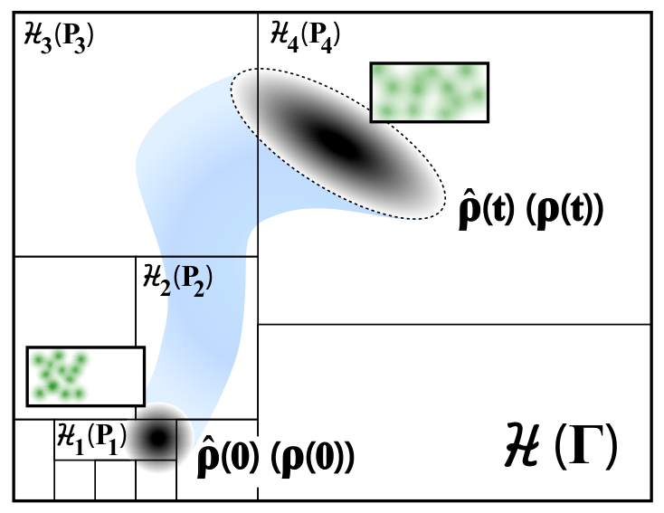


In contrast to equilibrium entropy, non-equilibrium thermodynamic entropy should not depend on the globally measured parameters of the system, but on the parameters measured locally, which brings in dependence on the non-equilibrium features of the state of the system. Additionally, it should correspond to the equilibrium value when the system is in equilibrium (see Fig. 2). Assuming that an experimentalist can measure energies and particle numbers locally, the non-equilibrium thermodynamic entropy is defined as1818 18 Here we assume multipartite system . Each is a space of all quantum states that can occur within a spatial region of volume , and and correspond to a particle and energy measurement of this spatial region. Šafránek et al. 2019b; Šafránek et al. 2019c
| (19) |
(See Fig. 3.) Per Eq. (13), this entropy is additive on independent systems. For the special case of common eigenstates of local particle and energy operators, this entropy gives the sum of local microcanonical entropies:
| (20) |
In the long-time limit, assuming weakly interacting (so that interaction energy between subsystems is negligible) particle conserving (so that is constant) non-integrable (so it thermalizes well, because there are not infinitely many conserved quantities) Hamiltonian, non-equilibrium entropy converges to the equilibrium value,
| (21) |
This convergence holds up to some finite size and finite particle number effects (see the Appendix and Refs. Šafránek et al. 2019b; Šafránek et al. 2019c for details).
The limit acts as its approximate upper bound1919 19 Proven to be an approximate upper bound in weakly interacting systems Šafránek et al. 2019b., which together with Eq. (15) gives2020 20 Additional exact bounds are given by Eqs. (5), (6). When local Hamiltonians and local particle operators commute, , Eq. (6) provides two bounds: one connected to observational entropy with just local particle numbers, and one with local energies.
| (22) |
| Entropy | Type | Definition | Relationship | Details |
|---|---|---|---|---|
| Boltzmann entropy | C/T | special case: for , | ||
| Coarse-grained entropy | C | single coarse-graining: | Eq. (2) | |
| Observational entropy | C | Eq. (4) | ||
| Entropy of an observable/entropy | C | equal to when all | Eq. (3) | |
| of partition | ||||
| Shannon entropy | I | Eq. (1) | ||
| Relative entropy | I | Eq. (7) | ||
| Gibbs/Differential entropy | T/I | Eq. (8) | ||
| Von Neumann entropy | I | , | Eq. (5) | |
| Entanglement entropy | I | Eq. (14) | ||
| Equilibrium thermodynamic entropy | T | Eq. (17) | ||
| Microcanonical, canonical, | T | Eq. (17) | ||
| grandcanonical entropy | for example | Eq. (18) | ||
| Non-equilibrium thermodynamic | T | , | Eq. (19) | |
| entropy | ||||
| Quantum correlation entropy/ | I | Eq. (14) | ||
| relative entropy of quantum discord/ | ||||
| zero-way quantum deficit |
The non-equilibrium thermodynamic entropy therefore describes the dynamical process of thermalization: starting as the sum of local entropies of independent subsystems, and after these subsystems start to interact, it grows to the global equilibrium entropy as the system thermalizes. It also has a very intuitive and compelling operational interpretation: At some intermediate time (when the system has only partially equilibrated) its value can be interpreted as the equilibrium thermodynamic entropy the system would attain in the long-time limit if (hypothetically) starting from time the subsystems were not allowed to exchange either energy or particles Šafránek et al. 2019c.
In non-equilibrium thermodynamic entropy, the choice of coarse-graining depends partially on the observer. It is the observer who chooses the partitioning into smaller subsystems, and then the coarse-graining is given by Hamiltonians of the subsystems themselves. The observer’s choice, however, would be naturally informed: it makes more sense to separate a joint system of a melting ice cube in a cup of water into a subsystem of ice and a subsystem of water. While other partitions are equally valid,2121 21 For example the first half of ice and the first half of water would together form the first subsystem, while the rest would form the second subsystem. they might not properly describe the process of a melting ice: the initial value of entropy could be quite large (close to the limit imposed by the equilibrium entropy), thus growing very little before achieving its maximum.
Finally, let us move into complete generality. In Eq. (17), the particle and energy coarse-graining has been chosen because it is standard for systems to conserve particle numbers, and this definition corresponds to the standard notions of equilibrium entropy. In general, there can be any number of conserved quantities (observables) in the system (typically one of them being energy). Having these conserved quantities, we define equilibrium entropy as
| (23) |
By definition, this expression stays constant in time. The non-equilibrium entropy can be then defined using local versions of these observables, as
| (24) |
It is expected that in weakly interacting isolated systems, the non-equlibirum entropy will grow to the equilibrium entropy as the system thermalizes. Interpretation follows the same pattern: non-equilibrium entropy is the value of entropy the isolated system would achieve in the long-time limit, if the subsystems were not allowed to exchange any of the values of the observables. For example, observable cannot flow from subsystem to subsystem , meaning that the mean values (and the probability distributions) of and remain constant.
There are several other coarse-grainings and corresponding observational entropies that could be considered, each with a different intepretation. For those, please see the Appendix, which also contains a few technical details and references.
VII Summary and Discussion
As discussed in the introduction, there are many types of entropy in physics; some entropies arise from information theoretic concepts, some from a type of coarse-graining, and some from a thermodynamic perspective.
Each of these entropies have a different purpose. Generally, an entropy can be considered a measure of missing information regarding the particular state of a system; different entropies measure different sources of such uncertainty. Given a closed system, lack of knowledge of the state of a system, the inability to distinguish different states of a system, and a restriction to measuring a subsystem of the system lead to, respectively, Gibbs/von Neumann, Boltzmann, and (in quantum systems) entanglement entropies. In turn, these relate in some sense to the thermodynamic entropy that is maximized in equilibrium, relates work/energy to temperature, and tends to rise in closed systems.
Observational entropy is primarily a coarse-graining based entropy which generalizes Boltzmann entropy to quantum systems. It depends on a density function or operator , a (vector of) coarse-graining(s) , and (potentially) a partitioning of the system into local subsystems. It is interpreted as the amount of information an observer would infer about the initial state of the system, if he or she were to perform a measurement in a basis given by the coarse-graining.
As summarized in this paper, the different senses of entropy outlined above can be both conceptually and mathematically unified in the framework of observational entropy. In particular, observational entropy transforms into other definitions of entropy given a special choice of coarse-graining or when minimizing over different types of coarse-grainings. This formalism allows for inclusion of multiple and even non-commuting coarse-grainings, and can be further generalized to POVMs and likely to other frameworks for describing acquisition of knowledge.
Some key results in quantum systems are:
- •
With a “fine” graining into individual states in an appropriate basis, yields the von Neumann entropy.
- •
For general coarse-grainings, is a form of Boltzmann entropy that is bounded below by the von Neumann entropy.
- •
For local coarse-grainings, is bounded by the sum of the von Neumann and the “quantum correlation entropy,” which generalizes entanglement entropy.
- •
The equilibrium thermodynamic entropy is given by coarse-grainings in global energy and global particle number (or by coarse-graining in other globally conserved quantities), and it generalizes other equilibrium entropies (such as microcanonical, canonical, and grand-canonical entropy).
- •
Non-equilibrium thermodynamic entropy is given by coarse-graining in local energy and local particle numbers, is additive on independent systems, and equal to the equilibrium entropy when the system is in equilibrium.
- •
Suitably applied to open systems, reduces to the standard formalism under the assumption of an infinite thermal bath.
See Table 1 for more relations between observational entropy and other quantities.
Various forms of the second law of thermodynamics emerge in observational entropy as they do in the more special special cases. Boltzmann entropy tends to rise (while occasionally fluctuating down) due to wandering of a system into higher-entropy macrostates; entanglement entropy tends to rise due to the forging of entanglement between two interacting subsystems; von Neumann entropy is forbidden from decreasing (or increasing) via information preservation in unitary dynamics; the total thermodynamic entropy tends to increase due to heat flowing from a warmer to a colder body. All of these effects are reflected in the dynamics of observational entropy.
Given the generality of this framework, we expect it will have many applications where its well-defined conceptual and mathematical underpinnings could bring clarity – for example in efficient discussion of the Gibbs paradox, in fluctuation theorems for both isolated and open quantum systems, in studying differences between thermalization of classical and quantum systems, in generalization of renormalization group methods to many-body systems in which quantum effects are important, and in systems with strong or long-range interactions (including gravity.)
Most broadly, it may be particularly useful in contexts in which the second thermodynamic law is used as a fundamental constraint on a total entropy that is a sum of different versions of entropy. This includes for example Maxwell’s demon and Szilard’s engine (and information engines in general, where Shannon and thermodynamic entropy are combined), the “generalized second laws” (where horizon and statistical entropy are combined), and in cosmology (where all manner of entropies are summed and assumed to increase). We hope that the observational entropy framework, which can accommodate many types, can be used to give more crisp and explicit mathematical and conceptual meaning to such arguments.
Acknowledgements.
This research was supported by the Foundational Questions Institute (FQXi.org), of which AA is Associate Director, and by the Faggin Presidential Chair Fund. DŠ acknowledges additional funding by the Institute for Basic Science in Korea (IBS-R024-Y2 and IBS-R024-D1).References
- Šafránek et al. (2019a) Dominik Šafránek, J. M. Deutsch, and Anthony Aguirre, “Quantum coarse-grained entropy and thermodynamics,” Phys. Rev. A 99, 010101 (2019a), arXiv:1707.09722 [quant-ph] .
- Šafránek et al. (2019b) Dominik Šafránek, J. M. Deutsch, and Anthony Aguirre, “Quantum coarse-grained entropy and thermalization in closed systems,” Phys. Rev. A 99, 012103 (2019b), arXiv:1803.00665 [quant-ph] .
- Šafránek et al. (2019c) Dominik Šafránek, Anthony Aguirre, and J. M. Deutsch, “Classical dynamical coarse-grained entropy and comparison with the quantum version,” eprint (2019c), arXiv:1905.03841 [cond-mat.stat-mech] .
- Strasberg (2019) Philipp Strasberg, “Entropy production as change in observational entropy,” eprint (2019), arXiv:1906.09933 [cond-mat.stat-mech] .
- Faiez et al. (2020) Dana Faiez, Dominik Šafránek, J. M. Deutsch, and Anthony Aguirre, “Typical and extreme entropies of long-lived isolated quantum systems,” Phys. Rev. A 101, 052101 (2020), arXiv:1908.07083 [quant-ph] .
- Strasberg and Winter (2020) Philipp Strasberg and Andreas Winter, “Heat, Work and Entropy Production in Open Quantum Systems: A Microscopic Approach Based on Observational Entropy,” eprint (2020), arXiv:2002.08817 [quant-ph] .
- Schindler et al. (2020) Joseph Schindler, Dominik Šafránek, and Anthony Aguirre, “Entanglement entropy from coarse-graining in pure and mixed multipartite systems,” arXiv e-prints , arXiv:2005.05408 (2020), arXiv:2005.05408 [quant-ph] .
- Riera-Campeny et al. (2020) Andreu Riera-Campeny, Anna Sanpera, and Philipp Strasberg, “Quantum systems correlated with a finite bath: nonequilibrium dynamics and thermodynamics,” arXiv e-prints , arXiv:2008.02184 (2020), arXiv:2008.02184 [quant-ph] .
- von Neumann (2010) John von Neumann, “Proof of the ergodic theorem and the h-theorem in quantum mechanics,” The European Physical Journal H 35, 201–237 (2010), https://arxiv.org/abs/1003.2133 .
- von Neumann (1955) John von Neumann, “Mathematical foundations of quantum mechanics,” (Princeton university press, 1955) pp. 410–416.
- Wehrl (1978) Alfred Wehrl, “General properties of entropy,” Rev. Mod. Phys. 50, 221–260 (1978).
- Gemmer and Steinigeweg (2014) Jochen Gemmer and Robin Steinigeweg, “Entropy increase in K-step Markovian and consistent dynamics of closed quantum systems,” Phys. Rev. E 89, 042113 (2014).
- Almheiri et al. (2020) Ahmed Almheiri, Thomas Hartman, Juan Maldacena, Edgar Shaghoulian, and Amirhossein Tajdini, “The entropy of Hawking radiation,” arXiv e-prints , arXiv:2006.06872 (2020), arXiv:2006.06872 [hep-th] .
- Latora and Baranger (1999) Vito Latora and Michel Baranger, “Kolmogorov-Sinai Entropy Rate versus Physical Entropy,” Phys. Rev. Lett. 82, 520–523 (1999), arXiv:chao-dyn/9806006 [nlin.CD] .
- Nauenberg (2004) Michael Nauenberg, “The evolution of radiation toward thermal equilibrium: A soluble model that illustrates the foundations of statistical mechanics,” American Journal of Physics 72, 313–323 (2004), arXiv:cond-mat/0305219 [cond-mat.stat-mech] .
- Kozlov and Treshchev (2007) V. V. Kozlov and D. V. Treshchev, “Fine-grained and coarse-grained entropy in problems of statistical mechanics,” Theoretical and Mathematical Physics 151, 539–555 (2007).
- Piftankin and Treschev (2008) G. Piftankin and D. Treschev, “Gibbs entropy and dynamics,” Chaos: An Interdisciplinary Journal of Nonlinear Science 18, 023116 (2008), https://doi.org/10.1063/1.2907731 .
- Županović and Kuić (2018) Paško Županović and Domagoj Kuić, “Relation between Boltzmann and Gibbs entropy and example with multinomial distribution,” Journal of Physics Communications 2, 045002 (2018), arXiv:1804.06818 [cond-mat.stat-mech] .
- Gell-Mann and Hartle (1993) Murray Gell-Mann and James B. Hartle, “Classical equations for quantum systems,” Phys. Rev. D 47, 3345–3382 (1993).
- Dowker and Kent (1996) Fay Dowker and Adrian Kent, “On the consistent histories approach to quantum mechanics,” Journal of Statistical Physics 82, 1575–1646 (1996), arXiv:gr-qc/9412067 [gr-qc] .
- Griffiths (2019) Robert B. Griffiths, “The consistent histories approach to quantum mechanics,” in The Stanford Encyclopedia of Philosophy, edited by Edward N. Zalta (Metaphysics Research Lab, Stanford University, 2019) summer 2019 ed.
- Farmer (1982) J. Doyne Farmer, “Information dimension and the probabilistic structure of chaos,” Zeitschrift für Naturforschung A 37, 1304 – 1326 (1982).
- Frigg (2004) Roman Frigg, “In what sense is the kolmogorov-sinai entropy a measure for chaotic behaviour?—bridging the gap between dynamical systems theory and communication theory,” The British journal for the philosophy of science 55, 411–434 (2004).
- Jost (2006) Jürgen Jost, Dynamical systems: examples of complex behaviour (Springer Science & Business Media, 2006).
- Daniel (1984) W Daniel, “The entropy of observables on quantum logic,” Reports on mathematical physics 19, 325–334 (1984).
- Anzà and Vedral (2017) F. Anzà and V. Vedral, “Information-theoretic equilibrium and observable thermalization,” Scientific Reports 7, 44066 (2017).
- Lent (2019) Craig S. Lent, “Quantum operator entropies under unitary evolution,” Phys. Rev. E 100, 012101 (2019), arXiv:1901.08956 [quant-ph] .
- Goldstein et al. (2019) Sheldon Goldstein, Joel L. Lebowitz, Roderich Tumulka, and Nino Zanghi, “Gibbs and Boltzmann Entropy in Classical and Quantum Mechanics,” eprint (2019), arXiv:1903.11870 [cond-mat.stat-mech] .
- Engelhardt and Wall (2019) Netta Engelhardt and Aron C. Wall, “Coarse graining holographic black holes,” Journal of High Energy Physics 2019, 160 (2019), arXiv:1806.01281 [hep-th] .
- Español et al. (1997) Pep Español, Mar Serrano, and Ignacio Zuñiga, “Coarse-graining of a fluid and its relation with dissipative particle dynamics and smoothed particle dynamic,” Int. J. Mod. Phys. C 08, 899–908 (1997), https://doi.org/10.1142/S0129183197000771 .
- Gao et al. (2017) Tong Gao, Meredith D. Betterton, An-Sheng Jhang, and Michael J. Shelley, “Analytical structure, dynamics, and coarse graining of a kinetic model of an active fluid,” Physical Review Fluids 2, 093302 (2017), arXiv:1703.00969 [cond-mat.soft] .
- Batchelor and Batchelor (1967) Cx K Batchelor and GK Batchelor, An introduction to fluid dynamics (Cambridge university press, 1967).
- Smith (1950) Joseph Mauk Smith, Introduction to chemical engineering thermodynamics (ACS Publications, 1950).
- Guggenheim (1956) E A Guggenheim, Statistical Thermodynamics; a Version of Statistical Mechanics for Students of Physics and Chemistry (The University press, 1956).
- Callen (1998) Herbert B Callen, Thermodynamics and an Introduction to Thermostatistics (AAPT, 1998).
- Fisher (1998) Michael E. Fisher, “Renormalization group theory: Its basis and formulation in statistical physics,” Rev. Mod. Phys. 70, 653–681 (1998).
- Kardar (2007a) Mehran Kardar, Statistical physics of particles (Cambridge University Press, 2007).
- Kardar (2007b) Mehran Kardar, Statistical physics of fields (Cambridge University Press, 2007).
- Ma (2018) Shang-Keng Ma, Modern theory of critical phenomena (Routledge, 2018).
- Wilson (1971) Kenneth G. Wilson, “Renormalization group and critical phenomena. i. renormalization group and the kadanoff scaling picture,” Phys. Rev. B 4, 3174–3183 (1971).
- Šafránek (2020) Dominik Šafránek, “Observational entropy with generalized measurements,” eprint (2020), arXiv:2007.07246 [quant-ph] .
- Polkovnikov (2011) Anatoli Polkovnikov, “Microscopic diagonal entropy and its connection to basic thermodynamic relations,” Annals of Physics 326, 486–499 (2011), arXiv:0806.2862 [cond-mat.stat-mech] .
- von Neumann (2010) J. von Neumann, “Proof of the ergodic theorem and the H-theorem in quantum mechanics. Translation of: Beweis des Ergodensatzes und des H-Theorems in der neuen Mechanik,” Eur. Phys. J. H 35, 201–237 (2010), arXiv:1003.2133 [physics.hist-ph] .
Appendix A Physically relevant coarse-grainings
In this appendix we collect and/or introduce, and discuss, a number of physically relevant coarse-grainings, generally with some relevance to thermodynamics, some of which have been studied in detail before von Neumann 2010; Šafránek et al. 2019a; Šafránek et al. 2019b; Šafránek et al. 2019c; Strasberg 2019; Strasberg and Winter 2020.
In terms of generic properties, any observational entropy generated by an observable (which is typically the case of (1) below) that is conserved in the system (i.e., commutes with the Hamiltonian) will be constant during the time evolution Šafránek et al. 2019b. Moreover, any entropy that consists solely of local coarse-grainings (which is the case of (2) below) will be additive on independent systems as per Eq. (13), and bounded as per (15). All convergence in the long-time limit discussed below in points (2) and (3) assumes particle conserving non-integrable2222 22 Although simulations Šafránek et al. 2019b show that integrable case also converges, just not that well. Hamiltonian with short range interactions, so that particles tend to thermalize well and the interaction energy between the subsystems is negligible. The convergence holds up to some corrections due to finite particle number and finite size-effect effects. These limits are approximate upper bounds for the non-equilibrium entropies, which is why we say “grows to.” The exact upper bounds follow from Eq. (6). For simplicity we also consider non-degenerate Hamiltonian (both globally and locally), which means that each energy has a unique associated particle number, so instead of common eigenstate of the particle operator and the Hamiltonian we can write simply . The two observational entropies discussed in the main body of this paper are (1c) and (2c).
(1a) Global particle number coarse-graining
Defining , where is a projector onto subspace of particles,
| (25) |
measures the uncertainty about the particle number in the system.
(1b) Global energy coarse-graining2323
23
This has been originally defined by von Neumann in von Neumann 2010, where he attributed this definition to Eugene Wigner. It was used extensively in both classical Šafránek et al. 2019c and quantum case Šafránek et al. 2019a; Šafránek et al. 2019b, usually as the value to which other entropies and (in case of fixed total number of particles) converge.
Defining , where is a projector onto subspace of wave functions within an energy shell (and is the coarse-grained Hamiltonian),
| (26) |
measures the equilibrium thermodynamic entropy of a system with a fixed number number of particles.
Details: is the resolution in energy of the measuring apparatus. If restricted to a Hilbert space with a fixed number of particles, for small but non-zero this entropy gives microcanonical entropy for both energy eigenstates and a microcanonical state, and it (approximately) gives Gibbs entropy for the Gibbs state . The case of cannot be applied to Hilbert space which includes variable number of particles, because the energy subspace would include wave-functions with any particle numbers, and would be typically infinite in size. For it does not have this problem (since energy eigenstate uniquely determines the particle number in common particle-conserving Hamiltonians), but it gives zero for energy eigenstates.
(1c) Global particle number with global energy coarse-graining
| (27) |
measures the equilibrium thermodynamic entropy.
Details: Macrostates now distinguish both energy and the number of particles, which means it can be used for systems with a variable number of particles. For common particle-conserving Hamiltonians, the case of reduces to . It gives microcanonical entropy, for a global energy eigenstate. is the spatial volume of the system.
(2a) Local particle number coarse-graining2424
24
Denoted in Šafránek et al. 2019b where its time evolution is illustrated in Fig. 2.
| (28) |
where are energies of the subsystems, and measures how uniformly are particles distributed over the subsystems.
Details: It grows to (1a) in the long-time limit: when particles spread uniformly throughout the system, they fill uniformly every particle shell.
(2b) Local energy coarse-graining2525
25
The case of has been studied in detail in Šafránek et al. 2019b under the name of “Factorized Observational entropy” or FOE for short, and denoted .
| (29) |
where are energies in the subsystems, how uniformly is energy distributed over the subsystems.
Details: For local energy eigenstates . Despite from what it may seem from (1b), for , does not describe thermodynamic entropy in each subsystem, because in a non-equilibrium system, number of particles in each subsystem typically varies, even though the total number of particles may be conserved. Macrostate contains all states with energy , even though these states might have different particle numbers. In case of Hamiltonians which conserve particles locally, each local eigenstate uniquely determines its particle number, which implies that the case of is identical to (2c), having all of its dynamical properties. However, for , , which is undesirable for a physically meaningful thermodynamic entropy. It grows to (1b) in the long-time limit.
(2c) Local particle number with local energy coarse-graining2626
26
This entropy has been studied closely in the classical case Šafránek et al. 2019c where it has been denoted , and where also the quantum equivalent is mentioned for the first time. Since in quantum case, this definition behaves the same (in its time evolution in particular) as (2b) for , apart from giving non-zero value for local energy eigenstates, we refer reader to Šafránek et al. 2019b for its detailed properties.
| (30) |
measures non-equilibrium thermodynamic entropy of the system.
Details: At some intermediate time (when the system has only partially equilibrated) its value can be interpreted as the equilibrium thermodynamic entropy the system would attain in the long-time limit if (hypothetically) starting from time the subsystems were not allowed to exchange either energy or particles Šafránek et al. 2019c. For , it gives , the sum of local microcanonical entropies, for a local energy eigenstate. denote the local spatial volumes. It grows to (1c) in the long-time limit.
(3a) Local particle number then global energy coarse-graining2727
27
This entropy has been studied in detail both in classical Šafránek et al. 2019c and quantum case Šafránek et al. 2019b where it was denoted .
| (31) |
is a different type of non-equilibrium thermodynamic entropy of the system.
Details: Is not additive. At some intermediate time , its value can be interpreted as the equilibrium thermodynamic entropy the system would attain in the long-time limit if (hypothetically) starting from time the subsystems were allowed to exchange energy but not particles Šafránek et al. 2019c. It is upper bounded by (2a), and it grows to (1c).
(3b) Global energy then local particle number coarse-graining2828
28
Time evolution of this entropy has been studied in the quantum case in Appendix H of Šafránek et al. 2019b, where it was denoted , but it was realized only later in Šafránek et al. 2019c that it has a meaningful interpretation. Classically, and are identical.
| (32) |
is similar in behavior to (3a), but differs when quantum effects become significant, such as at low energies and when subsystems are small so that effects of non-commutation between and intensify.
Details: It is upper bounded by (1b), and it grows to (1c). For , it is identical to (1b) and (1c).
(4) Combination of arbitrary local and local energy coarse-graining.2929
29
This entropy has been studied in detail by Strasberg and Winter in Strasberg 2019; Strasberg and Winter 2020.
| (33) |
is the total entropy of a small well-controlled subsystem plus large bath(s), with applications in open system non-equilibrium thermodynamics.
Details: Change in this entropy defines entropy production which, unlike the formulation based on von Neumann entropy, does not depend explicitly on the temperature(s) of the bath(s). Moreover, with this it is possible to define work as the part of the “useful” internal energy that can be recovered from the system, while heat is the part of internal energy that is irreversibly lost.