A Striped Electron Fluid on (111) KTaO3
Abstract
A recent study has revealed that the low carrier density electron gas (2DEG) induced at the interface of EuO and (111) KTaO3 exhibits a broken symmetry phase with a strong in-plane anisotropy of the resistivity. We present a minimal tight binding model of this (111) 2DEG, including the large spin-orbit coupling from the Ta ions, which reveals a hexagonal Fermi surface with a highly enhanced 2 electronic susceptibility. We argue that repulsive electronic interactions, together with a ferromagnetic EuO substrate, favor a magnetic stripe instability leading to a partially gapped Fermi surface. Such a stripe state, or its vestigial nematicity, could explain the observed transport anisotropy. We propose a theory for the low energy states, which captures the key results from our tight-binding study, and further reveals the intertwined dipolar and octupolar modulations underlying this magnetic stripe order. We conclude by speculating on the relation of this stripe order to the superconductivity seen in this material.
The superconducting 2DEG at the surface of SrTiO3 has been the subject of much investigation since its observation back in 2007 Reyren et al. 2007. A few years later, its analog, KTaO3 (KTO), was found to exhibit superconductivity (SC) at mK in an (001) 2DEG created using ionic liquid gating Ueno et al. 2011. A recent experiment discovered that for (111) oriented KTO, is dramatically enhanced, by a factor of 40, with SC occurring up to K at carrier densities /cm2 Liu et al. 2020. Even more remarkably, at low carrier densities where SC occurs with K, it descends from an apparent nematic phase with a significant in-plane resistance anisotropy of Liu et al. 2020. This anisotropy onsets abruptly at a higher temperature K, suggesting a phase transition into an ordered state. At zero magnetic field, the anisotropy is only observed if KTO is in contact with EuO (for KTO on LaAlO3, an in-plane magnetic field is required for its observation Liu et al. 2020). As EuO is ferromagnetic, magnetism is likely to play an important role in this phenomenon. The presence of charge, spin, and superconducting correlations as a function of carrier concentration for (111) KTO is reminiscent of a number of other materials such as cuprates Ando et al. 2002; Hinkov et al. 2008, iron pnictides and chalcogenides Paglione and Greene 2010, doped Bi2Se3 Matano et al. 2016; Yonezawa et al. 2017; Hecker and Schmalian 2018, and twisted bilayer graphene near a magic angle Cao et al. 2020. Furthermore, since the conduction band of KTO arises from spin-orbit coupled (SOC) states Mattheiss 1972; Bruno et al. 2019, the broken symmetry nematic is expected to also display intertwined multipolar orders as conjectured for Cd2Re2O7 Fu 2015; Harter et al. 2017; Di Matteo and Norman 2017; Hayami et al. 2019.

KTO is a band insulator with a large gap eV Jellison et al. 2006. Experiments have realized both a (001) 2DEG Nakamura and Kimura 2009; King et al. 2012; Santander-Syro et al. 2012; Zhang et al. 2019; Liu et al. 2020 and a (111) 2DEG Bareille et al. 2014; Bruno et al. 2019; Liu et al. 2020 at the free surface of KTO, due to oxygen vacancies induced by cleaving or by irradiating the surface, as well as at KTO interfaces with oxides such as LaAlO3 and EuO. Fig. 6 shows the crystal structure of (111) KTO, consisting of alternating layers of Ta and KO3, with each Ta layer forming a triangular lattice. This structure is highly polar given the nature of the Ta ions. Angle resolved photoemission spectroscopy (ARPES) of the 2DEG revealed six-fold symmetric Fermi surfaces (FSs) Bareille et al. 2014; Bruno et al. 2019. The observed bands were found to be captured by a (111) bilayer model Bareille et al. 2014, consisting of orbitals from two Ta layers forming a buckled honeycomb plane, a setting proposed for realizing topological phases by Xiao et al. Xiao et al. 2011.
We find that a minimal two-parameter honeycomb tight-binding model provides a good description of the ARPES observations; details can be found in sup and Refs. Xiao et al. 2011; Khalsa et al. 2013; Bruno et al. 2019; Liu et al. 2020. The dominant scale is the Ta-O-Ta hopping, eV, which is proportional to where is the hopping between the Ta and O orbitals, and is the Ta-O charge transfer energy. Since each Ta orbital hops to only two of the three nearest neighbors on the honeycomb lattice, the resulting bands exhibit 1D character. The FS of each orbital forms a spin-degenerate pair of parallel lines, with the FS of different orbitals rotated with respect to each other by 120 degrees sup. The inclusion of SOC, eV, which is the next largest energy scale, dramatically alters the electronic structure. SOC hybridizes the different 1D dispersions, and splits the manifold at the -point into a lower quartet and an upper doublet, separated by eV. The net result is that the parallel FS lines break up and reconstruct into closed FSs. Motivated by Ref. Bruno et al. 2019, we supplement this minimal model with a small trigonal distortion term so the quartet at splits into two Kramers doublets separated by meV. Our model provides a reasonable description of the recent ARPES data Bruno et al. 2019; sup, at a density /cm2, which reveals a larger outer star-shaped FS along with an inner hexagonal FS, both centered at 1su.
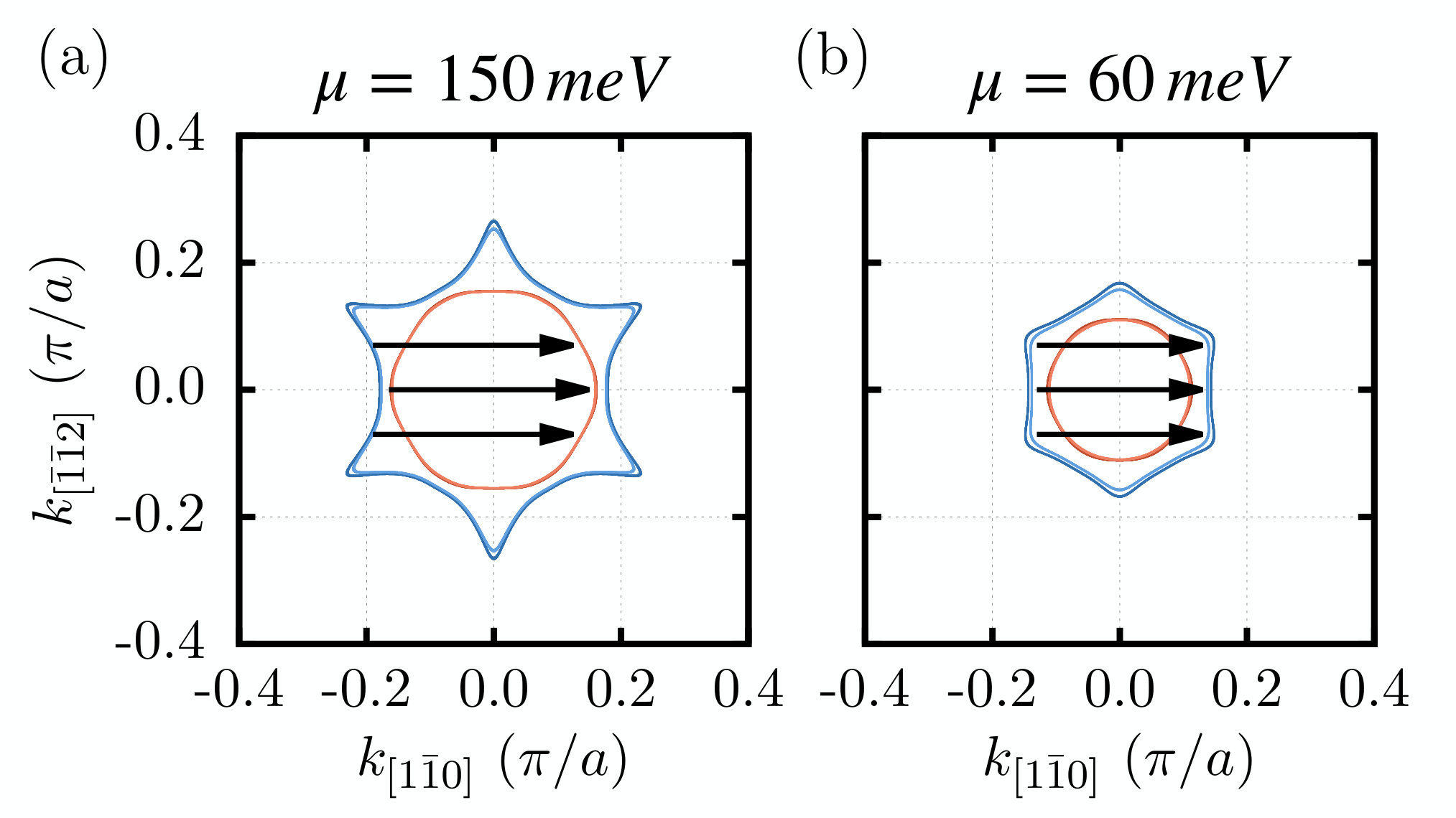
The recent experiments which observe nematic transport correspond to lower densities /cm2. To explore this regime, we start from our well-motivated model above, and lower the chemical potential to achieve this density. The resulting FS, shown in Fig. 6, reveals an inner circular FS, and an outer hexagonal FS which has flat faces nested along the - directions. We examine below the consequences of this nesting for stripe order and transport anisotropy. The FSs shown in Fig. 6 are spin-degenerate; we later incorporate weak Rashba spin splitting Bareille et al. 2014; Bruno et al. 2019 induced by the broken inversion symmetry at the interface.
The susceptibility for such a hexagonal FS is expected to resemble the 1D Lindhard function which diverges logarithmically in at the nesting wavevector. Interestingly, the nesting direction is along - (i.e., the (1,-1,0) direction) which corresponds precisely to the observed high resistivity direction in the nematic phase Liu et al. 2020. In a stripe model for the nematic phase, one would indeed anticipate that the resistivity is maximal along the stripe wavevector, . To investigate this further, we calculate the Lindhard susceptibility, , for the bilayer model:
| (1) |
where and are band indices, are Fermi functions, are the band energies, and is a small broadening (set to 0.1 meV or smaller). Although the bilayer model has six spin-degenerate pairs of bands (three orbitals, two layers), only the lowest two are relevant at low energy and we confine our discussion to them. To begin with, we will be agnostic concerning spin versus charge, and therefore not include matrix elements until later. The resulting , decomposed in terms of and , is shown in Fig. 2a. As expected, the outer hexagon gives rise to a susceptibility maximum along - due to nesting of each of the two parallel sides of the hexagon (as indicated in Fig. 6c). This is evident from the cusp-like behavior of the intraband , indicating quasi-1D behavior. Fig. 2b shows that this cusp becomes better defined upon lowering , as expected.
To proceed further, we need to consider matrix elements. In the experiments, the nematic phase at zero magnetic field is found at the KTO-EuO interface, but not at the KTO-LaAlO3 interface. This indicates that magnetism is playing a key role. This can be understood from the fact that the Eu electrons exhibit ferromagnetic order with a large moment. These electrons overlap with the Eu orbitals which in turn overlap with the Ta electrons (the Ta to oxide layer spacing in (111) KTO is only 1.15 Å, whereas Å, Å, and Å Desclaux 1973). Calculations for (001) EuO-KTO find induced moments of 0.2 on the first TaO2 layer Zhang et al. 2018. This motivates including spin matrix elements in the numerator of Eq. 1:
| (2) |
where , are spin- operators (=), and are the band eigenvectors. Because of strong SOC, the susceptibility is anisotropic even without the feedback from the energy gap due to density wave formation. The results are shown in Fig. 2c. The cusp along - is associated with the component of . As is orthogonal to (1,-1,0), this implies a transverse spin density wave, which is typical for a magnetic stripe model 2su.
The mean field transition temperature is determined by the divergence of the full interacting susceptibility. This is given by the condition , where is the interaction function. Based on the above considerations, we expect would be induced by the combined effect of the amorphous ferromagnetic EuO substrate and local Ta correlations, rendering it a weak function of . Thus, the ordering vector would be determined by the cusp in . The value of would need to be sizable (on the scale of eV) in order to induce the transition, with the low value of due to the logarithmic (BCS-like) rise in the cusp of with decreasing as can be seen in Fig. 2b. In this scenario, the disappearance of nematicity in higher carrier density samples could be due to the reduction of from screening, or due to enhanced disorder scattering as reflected by the lower mobility of such samples Liu et al. 2020.

We next consider the question of transport anisotropy in this stripe state. In Fig. 9, we show the outer FS as reconstructed by a spin-density wave within a simple calculation Norman et al. 2007 involving a secular matrix where one couples the states and with , with from the lowest band (band ) and a stripe potential, . Here, we take , and to have a typical mean-field value of 2 where K from Ref. Liu et al. 2020. We find that the original FS is wiped out along the nesting direction, leading to a reconstructed open FS which is expected to exhibit a strong resistive anisotropy.
We briefly comment on the energetic competition between a single- state versus a triple- state. In the presence of SOC, for a fixed spin direction, only one of the three equivalent - directions would have a cusp, but not the other two (as in Fig. 2c), leading to transport nematicity. Based on the above FS reconstruction, one might expect that a triple- state would gap out the entire outer FS (i.e., all hexagonal faces), and thus would be energetically preferred over the single- one. Such a state would not have an in-plane transport anisotropy. However, such non-coplanar spin crystals typically arise for a non-zero perpendicular magnetization whereas the EuO magnetization is expected to be in the plane of the interface. In this case, SOC could favor the single- state, with the moment direction locked to the stripe wavevector. This provides further support of a magnetic stripe rather than a charge stripe order. A complete treatment of this problem would require calculating the cubic and quartic terms in a Landau free-energy expansion McMillan 1975; Melikyan and Norman 2014, but this time including the spin matrix elements. This is an involved task, which we defer to future work.
We next consider the effect of the Rashba spin splitting. In a single-layer model, the Rashba term for the (111) case is given in Ref. Boudjada et al. 2018. As the Ta-Ta hopping in-plane is weak, we instead consider the Rashba term given by the Ta-O-Ta path connecting the layers, which is a (111) generalization of the (001) case considered by Khalsa et al. Khalsa et al. 2013. Here, the largest term is due to inversion breaking on one of the Ta-O segments followed by a hop along the other. The functional form is given in sup. Both this form and the one of Ref. Boudjada et al. 2018, which are off-diagonal in the orbital index, give similar results, with a relatively isotropic Rashba splitting around the FS (Fig. 8a). The effect of this is minor for without matrix elements given the small value of the Rashba splitting (of order a few meV). However, once we include their effect, the largest contribution comes from the interband component associated with the Rashba-split outer FS (Fig. 8b), which can be understood from the Rashba-induced FS spin texture.
While our tight-binding model study captures the salient observations for the (111) KTO 2DEG, it is nevertheless useful to construct a continuum theory for the low energy states near the -point Luttinger 1956; Venderbos et al. 2018. This allows us to clearly expose the multipolar character of the magnetic stripe order. We begin with a minimal 3D Luttinger model sup, , with eV, which reasonably captures the bulk band dispersion up to a momentum cutoff which we fix as (momenta are in units of the inverse cubic lattice constant ). Here, refer to spin- angular momentum operators (with ), and denotes the identity matrix. To describe the 2DEG, we project to 2D so that
| (3) |
with being momenta respectively along the and directions. To describe the hexagonal FS, we include the symmetry-allowed sixth-order terms,
| (4) | |||||
where and . We set eV; although naively appear to be large energy scales, note that for relevant densities. Finally, we incorporate two weaker terms: a trigonal distortion , and a Rashba coupling from inversion breaking,
| (5) |
where , , and we fix meV. Our model for the (111) 2DEG, , reasonably reproduces the tight-binding FSs from low to moderate densities sup.
The susceptibility matrix for this model involves the full set of multipole operators constructed from the quartet. In addition to dipole operators , this includes five quadrupoles (triplet: , doublet: ) and seven octupoles (singlet: , triplets: and ); see sup for the table of operators. We find that the susceptibility restricted to only the dipole operators reproduces the behavior shown in Fig. 4b sup. Fig. 5a shows the largest eigenvalue of the full matrix susceptibility, for both intraband and interband cases, for momentum along the nesting - direction. The strongest response still occurs for the interband between the two spin-split FSs. The key difference is that the intraband also show strongly enhanced, but nevertheless subdominant, peaks. Fig. 5b plots the magnitude of the eigenvector components of for the different multipoles at the peak momentum, showing that the symmetry breaking corresponds to intertwined magnetic dipolar and octupolar orders. As a consequence, the 2DEG stripe should exhibit modulated loop currents from octupolar order Paramekanti et al. 2020; Voleti et al. 2020.
We conclude with a discussion of the implications of our work. Given the involvement of EuO, and the fact that a magnetic stripe model gives a more natural explanation for a single- state than a charge-only model, we conclude that the ‘nematic’ phase seen by Liu et al. Liu et al. 2020 below K is a magnetic stripe. Experiments such as linear optical dichroism, Raman scattering, and resonant x-ray diffraction could shed further light on the nature of this broken symmetry state at the interface. The vestigial nematicity associated with the stripe order is expected to have relatively longer range correlations Nie et al. 2017; Fernandes et al. 2019, so it is likely to be pinned by the device geometry. The magnetic stripe state should also strongly impact the SC order. The gapped FS shown in Fig. 3 will reduce the number of states available for pairing, resulting in a lower in samples which exhibit nematicity. In addition, it will cause the SC itself to be anisotropic. Furthermore, for a spin-density wave state, the pairing in a paramagnetic basis can be written as a linear combination of a spin singlet at (here, refers to the center of mass momentum of the pair), and one component of a spin triplet at the magnetic wavevector, Fenton 1984. As such, the superconducting state will also exhibit spatial modulation, similar to a pair density wave state Agterberg et al. 2020, as suggested by Liu et al. Liu et al. 2020. A full treatment of the pairing problem would involve explicitly considering the Rashba splitting, given that its value exceeds both and . Finally, the increase of with carrier density could be due to the suppression of the magnetic stripe phase. This competition is commonly observed in density wave materials such as CuxTiSe2 Morosan et al. 2006.
The authors thank Anand Bhattacharya, Changjiang Liu and Ivar Martin for discussions. This work was supported by the Materials Sciences and Engineering Division, Basic Energy Sciences, Office of Science, U. S. Dept. of Energy. AP acknowledges funding from NSERC of Canada.
References
- Reyren et al. (2007) N. Reyren, S. Thiel, A. D. Caviglia, L. F. Kourkoutis, G. Hammerl, C. Richter, C. W. Schneider, T. Kopp, A.-S. Rüetschi, D. Jaccard, M. Gabay, D. A. Muller, J.-M. Triscone, and J. Mannhart, Science 317, 1196 (2007).
- Ueno et al. (2011) K. Ueno, S. Nakamura, H. Shimotani, H. Yuan, N. Kimura, T. Nojima, H. Aoki, Y. Iwasa, and M. Kawasaki, Nature Nanotechnology 6, 408 (2011).
- Liu et al. (2020) C. Liu, X. Yan, D. Jin, Y. Ma, H.-W. Hsiao, Y. Lin, T. M. Bretz-Sullivan, X. Zhou, J. Pearson, B. Fisher, et al., arXiv preprint arXiv:2004.07416 (2020).
- Ando et al. (2002) Y. Ando, K. Segawa, S. Komiya, and A. N. Lavrov, Phys. Rev. Lett. 88, 137005 (2002).
- Hinkov et al. (2008) V. Hinkov, D. Haug, B. Fauqué, P. Bourges, Y. Sidis, A. Ivanov, C. Bernhard, C. T. Lin, and B. Keimer, Science 319, 597 (2008).
- Paglione and Greene (2010) J. Paglione and R. L. Greene, Nature Physics 6, 645 (2010).
- Matano et al. (2016) K. Matano, M. Kriener, K. Segawa, Y. Ando, and G.-q. Zheng, Nature Physics 12, 852 (2016).
- Yonezawa et al. (2017) S. Yonezawa, K. Tajiri, S. Nakata, Y. Nagai, Z. Wang, K. Segawa, Y. Ando, and Y. Maeno, Nature Physics 13, 123 (2017).
- Hecker and Schmalian (2018) M. Hecker and J. Schmalian, npj Quantum Materials 3, 1 (2018).
- Cao et al. (2020) Y. Cao, D. Rodan-Legrain, J. M. Park, F. N. Yuan, K. Watanabe, T. Taniguchi, R. M. Fernandes, L. Fu, and P. Jarillo-Herrero, arXiv preprint arXiv:2004.04148 (2020).
- Mattheiss (1972) L. F. Mattheiss, Phys. Rev. B 6, 4718 (1972).
- Bruno et al. (2019) F. Y. Bruno, S. McKeown Walker, S. Riccò, A. de la Torre, Z. Wang, A. Tamai, T. K. Kim, M. Hoesch, M. S. Bahramy, and F. Baumberger, Advanced Electronic Materials 5, 1800860 (2019).
- Fu (2015) L. Fu, Phys. Rev. Lett. 115, 026401 (2015).
- Harter et al. (2017) J. W. Harter, Z. Y. Zhao, J.-Q. Yan, D. G. Mandrus, and D. Hsieh, Science 356, 295 (2017).
- Di Matteo and Norman (2017) S. Di Matteo and M. R. Norman, Phys. Rev. B 96, 115156 (2017).
- Hayami et al. (2019) S. Hayami, Y. Yanagi, H. Kusunose, and Y. Motome, Phys. Rev. Lett. 122, 147602 (2019).
- Jellison et al. (2006) G. E. Jellison, I. Paulauskas, L. A. Boatner, and D. J. Singh, Phys. Rev. B 74, 155130 (2006).
- Nakamura and Kimura (2009) H. Nakamura and T. Kimura, Phys. Rev. B 80, 121308 (2009).
- King et al. (2012) P. D. C. King, R. H. He, T. Eknapakul, P. Buaphet, S.-K. Mo, Y. Kaneko, S. Harashima, Y. Hikita, M. S. Bahramy, C. Bell, Z. Hussain, Y. Tokura, Z.-X. Shen, H. Y. Hwang, F. Baumberger, and W. Meevasana, Phys. Rev. Lett. 108, 117602 (2012).
- Santander-Syro et al. (2012) A. F. Santander-Syro, C. Bareille, F. Fortuna, O. Copie, M. Gabay, F. Bertran, A. Taleb-Ibrahimi, P. Le Fèvre, G. Herranz, N. Reyren, M. Bibes, A. Barthélémy, P. Lecoeur, J. Guevara, and M. J. Rozenberg, Phys. Rev. B 86, 121107 (2012).
- Zhang et al. (2019) H. Zhang, X. Yan, X. Zhang, S. Wang, C. Xiong, H. Zhang, S. Qi, J. Zhang, F. Han, N. Wu, B. Liu, Y. Chen, B. Shen, and J. Sun, ACS Nano, ACS Nano 13, 609 (2019).
- Bareille et al. (2014) C. Bareille, F. Fortuna, T. Rödel, F. Bertran, M. Gabay, O. H. Cubelos, A. Taleb-Ibrahimi, P. Le Fevre, M. Bibes, A. Barthélémy, et al., Scientific Reports 4, 3586 (2014).
- Xiao et al. (2011) D. Xiao, W. Zhu, Y. Ran, N. Nagaosa, and S. Okamoto, Nature Communications 2, 1 (2011).
- (24) See the Supplemental Material for details of the (i) bilayer tight-binding model, (ii) symmetry analysis leading to model and its Fermi surfaces, table of multipolar operators, and additional susceptibility plots.
- Khalsa et al. (2013) G. Khalsa, B. Lee, and A. H. MacDonald, Phys. Rev. B 88, 041302 (2013).
- (26) These two bands refer to the lowest subset of bands in quantum well language. There is weak evidence from ARPES for higher level sub-bands, but as these are over meV higher in energy, they play no role in regards to the low energy physics discussed here.
- Desclaux (1973) J. Desclaux, Atomic data and nuclear data tables 12, 311 (1973).
- Zhang et al. (2018) H. Zhang, Y. Yun, X. Zhang, H. Zhang, Y. Ma, X. Yan, F. Wang, G. Li, R. Li, T. Khan, Y. Chen, W. Liu, F. Hu, B. Liu, B. Shen, W. Han, and J. Sun, Phys. Rev. Lett. 121, 116803 (2018).
- (29) The Zeeman splittings of were not included in the calculations. Also note that in Figs. 2c and 4b, we plot the diagonal elements of the 3 by 3 spin matrix. We find this diagonal approximation is a good one for the maximum (i.e., ) eigenvalue. Moreover, in Fig. 2c, an implicit sum has been done over the Kramers degeneracy. That is 11 stands for 11+12+21+22, etc.
- Norman et al. (2007) M. R. Norman, A. Kanigel, M. Randeria, U. Chatterjee, and J. C. Campuzano, Phys. Rev. B 76, 174501 (2007).
- McMillan (1975) W. L. McMillan, Phys. Rev. B 12, 1187 (1975).
- Melikyan and Norman (2014) A. Melikyan and M. R. Norman, Phys. Rev. B 89, 024507 (2014).
- Boudjada et al. (2018) N. Boudjada, G. Wachtel, and A. Paramekanti, Phys. Rev. Lett. 120, 086802 (2018).
- Luttinger (1956) J. M. Luttinger, Phys. Rev. 102, 1030 (1956).
- Venderbos et al. (2018) J. W. F. Venderbos, L. Savary, J. Ruhman, P. A. Lee, and L. Fu, Phys. Rev. X 8, 011029 (2018).
- Paramekanti et al. (2020) A. Paramekanti, D. D. Maharaj, and B. D. Gaulin, Phys. Rev. B 101, 054439 (2020).
- Voleti et al. (2020) S. Voleti, D. D. Maharaj, B. D. Gaulin, G. Luke, and A. Paramekanti, Phys. Rev. B 101, 155118 (2020).
- Nie et al. (2017) L. Nie, A. V. Maharaj, E. Fradkin, and S. A. Kivelson, Phys. Rev. B 96, 085142 (2017).
- Fernandes et al. (2019) R. M. Fernandes, P. P. Orth, and J. Schmalian, Annual Review of Condensed Matter Physics 10, 133 (2019), https://doi.org/10.1146/annurev-conmatphys-031218-013200 .
- Fenton (1984) E. W. Fenton, Progress of Theoretical Physics Supplement 80, 94 (1984).
- Agterberg et al. (2020) D. F. Agterberg, J. S. Davis, S. D. Edkins, E. Fradkin, D. J. Van Harlingen, S. A. Kivelson, P. A. Lee, L. Radzihovsky, J. M. Tranquada, and Y. Wang, Annual Review of Condensed Matter Physics 11, 231 (2020).
- Morosan et al. (2006) E. Morosan, H. W. Zandbergen, B. S. Dennis, J. W. G. Bos, Y. Onose, T. Klimczuk, A. P. Ramirez, N. P. Ong, and R. J. Cava, Nature Physics 2, 544 (2006).
- Shiina et al. (1998) R. Shiina, O. Sakai, H. Shiba, and P. Thalmeier, Journal of the Physical Society of Japan 67, 941 (1998), https://doi.org/10.1143/JPSJ.67.941 .
- Chen et al. (2010) G. Chen, R. Pereira, and L. Balents, Phys. Rev. B 82, 174440 (2010).
Appendix A Tight-binding model
The bilayer model for KTaO3 (KTO) oriented along the (111) direction consists of three orbitals and two layers Xiao et al. 2011. Including the spin-orbit coupling, , the secular matrix is of order 12. We use the basis , , , , , , , , , , , , where indices label the layers. For purposes here, we only consider the largest hopping term, , which is diagonal in the orbital index, but off-diagonal in the layer index. The secular matrix has the following form:
| (6) |
where we define:
| (7) |
Here, and refer to orthogonal momenta in the hexagonal surface Brillouin zone (BZ), with being the projection of the bulk lattice constant, , onto the (111) plane (i.e., with Å). The in-plane (111) lattice constant is , which sets the scale for the surface BZ. We chose eV which, in the absence of other terms, fixes the total bandwidth of the model to (the value of being set by the bulk KTO bandwidth). The SOC term for orbitals has a value of 265 meV, leading to a bare quartet-singlet splitting of 397.5 meV at (i.e., when is turned off). This value has been chosen to match the large spin-orbit splitting reported from ab initio calculations of KTO Bruno et al. 2019. In addition, a small on-site trigonal distortion ( meV) is included that is off-diagonal in the orbital index. With the other terms turned off, this leads to a 15 meV splitting at . We have found that the other (smaller) hoppings, as well as the potential difference between the two layers, which were considered in Ref. Xiao et al. 2011, play only a minor role and are not included here.
The -only model generates a Fermi surface consisting of three pairs of parallel lines along each the - direction (Fig. 6a), which are perfectly nested along -. Once spin-orbit coupling is included, the band structure changes and the flat band in the -only model becomes dispersive as seen in Fig. 6b. With this model, we have performed calculations at two densities (set by the chemical potential), a higher one to match the ARPES results Bruno et al. 2019, and a lower one to match that of Liu et al. Liu et al. 2020. These two densities give rise to different Fermi surfaces (Figs. 6c and 6d). For the higher density, the outer pocket has a star-like shape and the inner pocket has a hexagonal shape. In this case, the maximum in the susceptibility does not come along - (due to nesting of the outer star surface), but rather along - due to nesting between the outer and inner surfaces. However, in the lower density case, the outer surface becomes hexagonal, and the maximum in the susceptibility is due to nesting along - for the outer surface, as shown in the main text.
Appendix B Rashba Term
The Rashba term can be derived by generalizing the work of Khalsa et al. Khalsa et al. 2013 to the (111) case. As (111) is parallel to , more terms enter than in their (001) case. As an example, the to hopping along the Ta-O-Ta cubic direction is of the form where the first matrix element is , with the overlap integral between Ta and O orbitals, and the second one is the inversion breaking term due to the electric field along the direction, . This results in the following matrix elements, , to be added to the secular matrix:
| (8) |
where diagonality in the spin index is implicit. (Note that this corresponds to an orbital inversion symmetry breaking and is thus spin-diagonal.) The spin-splitting arises from the combination of this inversion breaking term and the atomic SOC. We have found that a value of of 2 meV is needed to reproduce the suggested Rashba splitting along - of Bruno et al. Bruno et al. 2019. This value leads to an almost uniform splitting of around 0.005 for the outer surface of the lower density case of Liu et al. Liu et al. 2020.
Appendix C j=3/2 effective model and multipoles
For a cubic crystal, the symmetry-allowed continuum 4-band Luttinger model for the 3D bulk dispersion near the -point is given, to , by
| (9) |
Here, refer to spin- angular momentum operators (with ), is the identity matrix, and we measure momenta in units of where Å is the cubic lattice constant. For KTaO3, we find that a single parameter model, with and eV, captures the band dispersion near the point. We impose a momentum cutoff .
To describe the 2DEG, we take this dispersion and project it to 2D, expressing it in terms of orthogonal momentum components in the plane of the 2DEG, namely and which are respectively along the and directions, so , , and . The projected 2D Hamiltonian is
| (10) |
Going beyond these terms which descend from the bulk dispersion, we need to incorporate additional symmetry allowed terms in order to describe the 2DEG dispersion. We begin by considering mirror symmetry , time reversal , three-fold rotation , and inversion , and then incorporate Rashba terms from breaking . For convenience, we define . Under lattice symmetry operations, the momenta and transform as:
If inversion and time-reversal are unbroken, cubic terms in the momenta are ruled out, and the next important terms which we find capture the hexagonal shape of the 2DEG dispersion are sixth order terms in momenta,
| (20) | |||||
where . Finally, we incorporate two weaker terms: an effective trigonal distortion , and a Rashba coupling from inversion breaking, via
| (21) |
where and . We set eV, and fix the weaker terms to be meV in order to match the tight-binding results for the spin splitting of the FSs and the splitting of the quartet at the -point. This Hamiltonian may be viewed as a simple continuum model for the KTaO3 (111) 2DEG for low to moderate dopings. The Fermi surfaces from this Hamiltonian are shown in Fig. 7, and are in reasonable agreement with the FSs from the tight-binding model discussed in the main text.
The multipole moments within the quartet are given in the table below. We have normalized these multipole operators such that . This normalization is chosen such that the dipole operator matrices are simply the usual matrices. Different normalization schemes, as in Refs. Shiina et al. 1998; Chen et al. 2010, would lead to quantitative changes in the susceptibility results in the main text, but the key conclusions, that the dominant eigenvalue of stems from interband (12+21) nesting, and that it involves dipoles and octupoles, remains robust.
| Multipole | Symmetry | Operator |
|---|---|---|
| Dipole | ||
| Quadrupole | ||
| Octupole | ||
In order to compare these results with the results from the tight-binding model calculations, we also plot in Fig. 8 the susceptibility eigenvalues for intraband and interband orders when we truncate the susceptibility matrix to just the dipole operators, where we find qualitative agreement with the results from Fig. 4 of the main text.
Fig. 9a-f shows the real and imaginary components of the eigenvectors corresponding to the peaks in shown in the main text where we diagonalize the full susceptibility matrix.