Two-stage building energy consumption clustering based on temporal and peak demand patterns

Milad Afzalan Farrokh Jazizadeh and Hoda Eldardiry

Abstract

Analyzing smart meter data to understand energy consumption patterns helps utilities and energy providers perform customized demand response operations. Existing energy consumption segmentation techniques use assumptions that could result in reduced quality of clusters in representing their members. We address this limitation by introducing a two-stage clustering method that more accurately captures load shape temporal patterns and peak demands. In the first stage, load shapes are clustered by allowing a large number of clusters to accurately capture variations in energy use patterns and cluster centroids are extracted by accounting for shape misalignments. In the second stage, clusters of similar centroid and power magnitude range are merged by using Dynamic Time Warping. We used three datasets consisting of $\mathchar 12824$ 250 households ( $\mathchar 12824$ 15000 profiles) to demonstrate the performance improvement, compared to baseline methods, and discuss the impact on energy management.

Index Terms:

Clustering methods, energy segmentation, demand response, smart meters, energy management.

I Introduction

Demand response (DR) mechanisms help electricity providers maintain distribution reliability, reduce generation cost and environmental concerns, and increase utilization of renewables. Residential sector accounts for $\mathchar 12824$ 40% of electricity consumption in the U.S. [1], making it a proper candidate for DR engagement [2]. It is challenging to efficiently implement DR due to the highly varied energy load shapes across buildings. It is therefore important to learn and predict consumer behavior. Advanced metering infrastructure (AMI) and smart meters have been adopted to provide fine-grained (hourly or sub-hourly) energy data for advanced analytics to enhance the efficiency of power network operations. Electricity load shapes segmentation from smart meters, through clustering techniques, could inform decision-makers about different patterns of energy use towards improving resource allocation in power systems [3, 4]. With the wide adoption of smart meters nationwide [5], and the availability of hourly and sub-hourly data, segmentation methods have been used to find similar patterns of electricity consumption behavior of customers. This task can be applied in different capacities to improve power system operation including DR programs implementation [6], load forecasting [7], tariff determination [8], and renewable integration [9, 10]. The primary objective of the customer segmentation task is to transform a large library of load shapes (i.e., all profiles in the database) into representative daily energy use routines, which altogether define the typical behaviors of the entire customer base.

A review of the literature shows that different efforts have mainly adopted clustering techniques and considered their output self-evident from an application standpoint, without further verification of how the resultant clusters properly reflect the actual energy behaviors. Specifically, averages of all profiles, associated with each cluster, have been treated as representations of a distinct energy use behavior, although the average representation may not properly represent the actual shapes of profiles in a cluster. This assumption could result in two problems: 1) the accuracy of the segmentation will be low and customers will be assigned to the clusters that do not reflect their energy behavior realistically, and 2) some of the representative energy use behaviors, which have considerable frequency in the database, might not be reflected in any of the clusters. As a result, certain characteristics that are important to the utilities and decision-makers in the process of load balancing and planning, including the distribution of relative peak demands in the load shapes and the magnitude of peaks, may not be reflected in the segmentation results.

Given these shortcomings, we introduced a segmentation approach that accounts for compatibility of consumption patterns across load shapes while capturing both temporal shapes and peak demands of usage profiles. We have proposed a two-stage clustering of daily electricity load shapes by initially overpopulating the set of clusters for preserving accuracy and further merging similar clusters by accounting for cluster shape alignment. Evaluation is done on real-world smart meter data using various metrics based on measuring error in clustering and correlation analysis. The key contributions of this work include (1) a proposed household electricity load shape segmentation for fine-grained representation of load profile patterns and peak demands, and (2) introducing quantified evaluation of segmentation quality, which improves on most prior efforts in power systems that considered the segmentation performance self-evident without investigating related assessment metrics.

The rest of the paper is organized as follows: section II presents the related work, section III defines the problem, section IV discusses the proposed approach, section V presents the results, and sections VI and VII conclude the paper.

II Related Work

The concept of load shapes segmentation has received increasing attention with the proliferation of smart meters. Initial efforts [11, 12] have leveraged clustering techniques for classifying customers based on their load shape patterns. Different algorithms, including K-means [6], Self-Organizing Map (SOM) [13], hierarchical clustering [14], and Expectation-Maximization (EM) [15] have been investigated for the task of customer segmentation across tens to hundreds of households [6, 16]. Several recent efforts in household electricity segmentation have focused on addressing specific applications. In a class of studies, the use of big data, and the efficiency of clustering at the city-scale have been investigated [17, 18]. Therefore, due to the increasing size of datasets, the applicability of dimensionality reduction techniques such as Principal Component Analysis (PCA) and Symbolic Aggregate Approximation (SAX) [4], in addition to feature extraction from the attributes of interests from load shapes (such as peak distributions or key timeframes) have been investigated [19, 9]. Furthermore, to mitigate the impact of noisy and unequal time-series with incomplete information in the real-world scenarios, the model-based approach, which accounts for the phase shift and time lag has been proposed [20]. In some recent attempts, investigation of segmentation on disaggregated (i.e., individual load level) data, including Air Conditioning (AC) has been carried out for DR applications [21, 22].

As a core assumption in household electricity segmentation and its potential applications, the clustering output (both in terms of cluster quality and the number of clusters) has been assumed to reasonably represent the energy behavior patterns of the entire customer base. Such an assumption has been deemed either as self-evident without further investigation [23], investigated through common cluster validation indices (CVI) [24, 4, 14], or justified through empirical inspection [17]. The application of common CVIs has been deemed to be viable for quality assessment of the clustering outcome at the first sight. Examples of typical CVIs include Bayesian Information Criterion (BIC) [25], Silhouette index [26], and Davies–Bouldin index (DBI) [27]. However, as outlined in [17], such generic statistical indicators for model selection will not necessarily work for the electricity segmentation task. In other words, proper metrics that indeed measure the compatibility of individual load shapes with their representative clusters with respect to their associated profiles have been mainly ignored in the evaluation processes [10].

As the trend in the literature shows, the household electricity segmentation efforts have mainly overlooked the importance of recovering nuances of load shapes with distinct temporal patterns. Therefore, in this work, we focused on the fine-grained load shape cluster representation with distinct temporal patterns and peak demand magnitude through two-stage segmentation.

III Preliminaries and Motivation

Due to the highly varied patterns of energy consumption across different households on a daily basis, the task of segmentation can become challenging. In this section, the problem statement is presented through a quantitative case-study. We first demonstrated how common cluster validation indices (CVIs) for segmentation can lead to coarse-level representation of load shapes. We further highlighted the importance of recovering distinct load shapes from the clustering process.

III-A Dataset description

In this study, we used the data from the Pecan Street Project [41], which is an ongoing campaign in energy-efficiency initiative through equipping residential buildings with metering devices. Here, we used a subset of a dataset that was collected from residential buildings in Austin, TX and Boulder, CO during July and August 2015. Table I presents the characteristics of the datasets. The resolution of data was one sample per 15-minute. Therefore, each daily profile contains 96 data points. The duration of data collection for each dataset was 60 days. Three datasets were considered to impose adequate variations in the energy consumption styles. However, since the households were primarily located in Austin, TX, we divided the households in that geographical locations into two datasets.

TABLE I: Characteristics of the dataset

Dataset	Location	Number of households	# of daily profiles
Dataset 1	Austin, TX	129	7535
Dataset 2	Austin, TX	100	5676
Dataset 3	Boulder, CO	31	1790

Figure 1 shows the distribution of total daily energy consumption for all observations in different datasets. The median energy consumption for dataset 1, dataset 2, and dataset 3 is 44 kWh, 42kWh, and 17kWh, respectively.

Fig. 1: Distribution of energy consumption among all profiles.

III-B Problem statement description

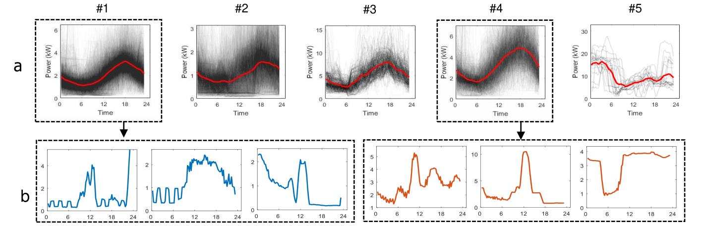
To demonstrate the problem in a generic form, a common clustering outcome on daily profiles has been presented. Figure 2 shows the clustering results of $\mathchar 12824$ 8000 daily load shapes clustered into 5 groups using K-means algorithm, which is commonly applied in the literature for the datasets of similar size and nature. In Figure 2(a), each subplot shows the temporal shape of each cluster, and the vertical axis is the power magnitude (in kW). The red line is the centroid of each cluster, which is obtained by averaging all daily profiles (in the order of hundreds or thousands) associated with the cluster. In Figure 2b, several examples of daily profiles associated with cluster 1 and 4 are shown. In the literature, the segmentation results were typically presented similar to what shown in Figure 2a, without further investigation of cluster quality. Therefore, the validity of clustering results were assumed as self-evident, and no further investigations were carried out to show how representative each cluster is with respect to its associated members. However, as shown in Figure 2b, examples of load shapes for #1 are retrieved that do not resemble the shape of its centroid. Similarly, a number of load shapes in cluster #4 are presented (Figure 2b) that do not resemble their cluster centroid (Figure 2a). Considering that these examples of load shapes in Figure 2(b) have considerable density in the entire dataset, it is important to have their own clusters to represent distinct energy behaviors. While one solution is to increase the number of clusters to allow for better representation of load shapes, this could come at the cost of obtaining a large number of clusters with high similarity, that contradicts the objective of segmentation. Based on this discussion, it could be seen that variations in temporal patterns of load shapes and their peak demands make the segmentation task challenging. Specifically, this problem becomes more important as the scope of segmentation gets larger both with higher number of households and historical days. Therefore, it is important to perform efficient segmentation on such datasets to allow for the trade-off between representing typical energy consumption patterns and maintaining interpretable number of clusters.

Refer to caption — Fig. 2: Segmentation of $\mathchar 12824$ 8000 load shapes using K-means: a) five clusters representing the entire dataset, b) examples of individual daily profiles for clusters 1 and 4 that are misclassified.

III-C Investigation of typical CVIs

Segmentation is commonly done using a small number of clusters. This is intuitive to ensure the ease of interpretation as a primary criterion for segmentation. To justify the number of clusters, cluster validation indices (CVIs) are commonly used. Here, to show the challenge of using typical CVIs and show the complexity in clustering patterns, we used several well-known CVIs, namely, the Davies-Bouldin Index (DBI) [27], Silhouette (SIL) [26], Calinski Harabasz (CH) [28], and Within Cluster Sum of Squared (WCSS) error [29]. CVIs definitions are provided in Table II.

TABLE II: CVI description.

CVI	Definition	Selection criterion	Ref
Davies Bouldin Index (DBI)	${{\mathchar 28721\over\mathchar 29003}}\mathchar 4944\displaylimits_{\mathchar 29033}\mathchar 29037\mathchar 29025\mathchar 29048_{\mathchar 29034\mathchar 24891\mathchar 29034\mathrel{{{{\mathchar 566\mathchar 61}}}}\mathchar 29033}\{{{{{\mathchar 28721\over\mathchar 12907\mathchar 28995_{\mathchar 29033}\mathchar 12907}}\mathchar 4944\displaylimits_{\mathchar 29048\mathchar 12850\mathchar 28995_{\mathchar 29033}}\mathchar 29028\delimiter 67273472\mathchar 29048\mathchar 24891\mathchar 28950_{\mathchar 29033}\delimiter 84054785\mathchar 8235{{\mathchar 28721\over\mathchar 12907\mathchar 28995_{\mathchar 29034}\mathchar 12907}}\mathchar 4944\displaylimits_{\mathchar 29048\mathchar 12850\mathchar 28995_{\mathchar 29034}}\mathchar 29028\delimiter 67273472\mathchar 29048\mathchar 24891\mathchar 28950_{\mathchar 29034}\delimiter 84054785\over\mathchar 29028\delimiter 67273472\mathchar 28950_{\mathchar 29033}\mathchar 24891\mathchar 28950_{\mathchar 29034}\delimiter 84054785}}\}$	Minimum	[27]
Silhouette (SIL)	${{\mathchar 28721\over\mathchar 29003}}\mathchar 4944\displaylimits_{\mathchar 29033}\{{{\mathchar 28721\over\mathchar 12907\mathchar 28995_{\mathchar 29033}\mathchar 12907}}\mathchar 4944\displaylimits_{\mathchar 29048\mathchar 12850\mathchar 28995_{\mathchar 29033}}{{\mathchar 29026\delimiter 67273472\mathchar 29033\delimiter 84054785\mathchar 8704\mathchar 29025\delimiter 67273472\mathchar 29033\delimiter 84054785\over\mathchar 29037\mathchar 29025\mathchar 29048\delimiter 67273472\mathchar 29026\delimiter 67273472\mathchar 29033\delimiter 84054785\mathchar 24891\mathchar 29025\delimiter 67273472\mathchar 29033\delimiter 84054785\delimiter 84054785}}\}$	Maximum	[26]
Calinski-Harabasz Index (CHI)	${{\mathchar 4944\displaylimits_{\mathchar 29033}\mathchar 12907\mathchar 28995_{\mathchar 29033}\mathchar 12907\mathchar 8707\mathchar 29028^{\mathchar 28722}\delimiter 67273472\mathchar 28950_{\mathchar 29033}\mathchar 24891\mathchar 28950_{\mathchar 29034}\delimiter 84054785\delimiter 68408078\delimiter 67273472\mathchar 29003\mathchar 8704\mathchar 28721\delimiter 84054785\over\mathchar 4944\displaylimits_{\mathchar 29033}\mathchar 4944\displaylimits_{\mathchar 29048\mathchar 12850\mathchar 28995_{\mathchar 29033}}\mathchar 29028^{\mathchar 28722}\delimiter 67273472\mathchar 29048\mathchar 24891\mathchar 28950_{\mathchar 29034}\delimiter 84054785\delimiter 68408078\delimiter 67273472\mathchar 29006\mathchar 8704\mathchar 29003\delimiter 84054785}}$	Maximum	[28]
Within Cluster Sum of Squared (WCSS)	$\mathchar 4944\displaylimits_{\mathchar 29033}\mathchar 4944\displaylimits_{\mathchar 29048\mathchar 12850\mathchar 28995_{\mathchar 29033}}\mathchar 12907\mathchar 29048\mathchar 8704\mathchar 28950_{\mathchar 29033}\mathchar 12907^{\mathchar 28722}$	Elbow	[29]

Notation: $\mathchar 29003$ : number of clusters; $\mathchar 28995_{\mathchar 29033}$ : Cluster $\mathchar 29033$ ; $\mathchar 12907\mathchar 28995_{\mathchar 29033}\mathchar 12907$ : Number of load shapes in $\mathchar 28995_{\mathchar 29033}$ ; $\mathchar 28950_{\mathchar 29033}$ : centroid of $\mathchar 28995_{\mathchar 29033}$ ; $\mathchar 29006$ : total number of load shapes; $\mathchar 29025\delimiter 67273472\mathchar 29048\delimiter 84054785\mathchar 12349{{\mathchar 28721\over\mathchar 12907\mathchar 28995_{\mathchar 29033}\mathchar 12907\mathchar 8704\mathchar 28721}}\mathchar 4944\displaylimits_{\mathchar 29034\mathchar 12850\mathchar 28995_{\mathchar 29033}\mathchar 24891\mathchar 29033\mathrel{{{{\mathchar 566\mathchar 61}}}}\mathchar 29034}\mathchar 29028\delimiter 67273472\mathchar 29033\mathchar 24891\mathchar 29034\delimiter 84054785$ , $\mathchar 29026\delimiter 67273472\mathchar 29048\delimiter 84054785\mathchar 12349\mathchar 29037\mathchar 29033\mathchar 29038_{\mathchar 29035\mathrel{{{{\mathchar 566\mathchar 61}}}}\mathchar 29033}{{\mathchar 28721\over\mathchar 12907\mathchar 28995_{\mathchar 29033}\mathchar 12907}}\mathchar 4944\displaylimits_{\mathchar 29034\mathchar 12850\mathchar 28995_{\mathchar 29035}}\mathchar 29028\delimiter 67273472\mathchar 29033\mathchar 24891\mathchar 29034\delimiter 84054785\mathchar 314$

We measured the CVIs for four common clustering methods (Self-Organizing Map (SOM), K-means, Fuzzy c-means,and hierarchical clustering). To choose the number of clusters ( $\mathchar 29003$ ), CVI is measured over a range of $\mathchar 29003$ values, and a selection criterion (Table II) is used on CVI values. We compared the range of $\mathchar 29003$ =5,10,15,20,…,120 to have a reasonable estimation of low to high number of clusters. We used 1 cluster increments in the commonly used range 5 to 10 (i.e., 5,6,7,8,9,10), and for more than 10, we used 5 cluster increments till $\mathchar 29003$ (end)=120 (i.e., 10,15,20,…,120). For each value of $\mathchar 29003$ , we cluster and measure CVIs. Figure 4 presents the CVIs for Dataset 1, with one subplot representing one CVI. The trend of increase/decrease for all 4 CVIs (each subplot) is almost consistent across datasets. Therefore, we presented the interpretation for Dataset 1 below, and the findings were consistent with other datasets as well. DBI metric uses a min-rule for selecting the proper $\mathchar 29003$ . As the results show, for all methods, a low value of $\mathchar 29003$ =5 leads to low DBI values. It must be noted that DBI values for fuzzy c-means showed to be very high. Therefore, we did not present its values in the first subplot to avoid masking the trend of changes for other methods. SIL metric uses a max-rule for selecting the $\mathchar 29003$ . Similar to the previous case, the lowest value of $\mathchar 29003$ =5 is estimated. CHI metric uses a max-rule for selecting the $\mathchar 29003$ . We select $\mathchar 29003$ =5 for this metric. However, for WCSS, that follows the elbow criterion for selecting the $\mathchar 29003$ , $\mathchar 29003$ =30 is a reasonable value for hierarchical, SOM, and K-means.

When it comes to algorithms, for DBI and SIL metrics, K-means shows a marginal improvement over SOM and hierarchical clustering. For CH metric, SOM and K-means show an equally better performance. For the WCSS metric, hierarchical clustering has the lowest values and seems to have a better performance. Therefore, there is no consistency in selecting a superior approach by considering combinations of CVIs and clustering algorithms. Nonetheless, to visually evaluate the performance of common algorithms based on optimum CVIs, an assessment of the clustering results is presented in the next section. Table III shows optimum $\mathchar 29003$ values, inferred based on CVIs for each dataset investigated in the next section.

Fig. 3: CVI for different clustering algorithms.

TABLE III: K values for different datasets and algorithms inferred by using the optimum CVIs.

Algorithm	K (Dataset 1)	K (Dataset 2)	K (Dataset 3)
K-means	5	8	6
HC, SOM	30	25	25

III-D Comparison of clustering results

Form cases in Table III, Figure 4 presents the clusters for dataset 1 as an example demonstration. Each subplot is one cluster, and the red curve is the cluster centroid, averaged over all profiles. The frequency value above each subplot shows the occurrence rate of the cluster within the entire dataset. In Figure 4(a), with $\mathchar 29003$ =5, four out of five clusters have peak demand around 18:00, but with different peak magnitudes. Cluster 5 seems to be an outlier, due to its considerable high peak usage in addition to its very low frequency (less than 1% of the data). In Figure 4(b) and Figure 4(c), with a higher population of clusters, more distinct energy patterns were revealed, while their presence has been masked by selecting a lower number in Figure 4(a). Examples include clusters 4, 11, and 17 in Figure 4(b), and clusters 8, 19, and 21 in Figure 4(c). Furthermore, a comparison between hierarchical clustering and SOM with equal number of clusters (Figure 4(b) and Figure 4(c)) show that hierarchical clustering emphasizes on identifying clusters with very low frequency (4 clusters with frequency of less than 0.5%) while SOM forms clusters with higher frequency. As shown in Figure 4, although CVI selects $\mathchar 29003$ =5, using such a low value will result in a very coarse-level representation of load shape groups. Specifically, the cluster centroids, which altogether are supposed to encompass the energy use behavior of the community, might not reflect the temporal shape/peak demands of their associated members.

Given the variations in the nature of CVIs, using different metrics results in selecting different $\mathchar 29003$ values for different algorithms. Generic CVIs might not work well for this domain-specific problem because several groups of energy patterns with distinct loads may not be recovered without selecting a large number of clusters, while their shapes/magnitude characteristics could be of interest to energy planners/utilities. Therefore, the next section introduces an approach to tackle this problem.

IV Two-stage clustering on household electricity load shapes

As discussed in Section III-D, optimizing the number of clusters on CVIs could result in an unreasonably low number of clusters. On the other hand, selecting a high number of clusters could improve the representation of various load shapes. However, it could affect the interpretation of the outcome due to presence of multiple correlated clusters. To account for this trade-off, a two-stage clustering approach is introduced that initially overpopulates clusters to improve the accuracy of load shape representations and further merge the closely related ones to improve the interpretability. The general framework is shown in Figure 5. The objective is to reduce the initial cluster library with fine-grained representation without losing the essential information in load shape patterns/peak demands. In the first stage, a large number of clusters is generated, which are then transformed with a time-series averaging technique to represent cluster centroids. In the second stage, pairwise distances of clusters are calculated with a distance measure that accounts for shape alignment between cluster centroids to merge the similar ones. Each component is described next.

Fig. 5: Two-stage clustering framework. Benchmark clustering is an arbitrary clustering technique (e.g., k-means). Acronyms: DBA (Dynamic Time Warping Barycenter Averaging); CIDTW (Complexity-Invariant Dynamic Time Warping).

IV-A First stage: Initial cluster representation

IV-A1 Overpopulation of clusters

To provide a diverse set of load shapes that captures a wide selection of the possible profiles, a representative of the true distribution of the profiles in the entire dataset is needed. In the first stage, an initial value of $\mathchar 29003^{{}^{\mathchar 560}}$ for the number of clusters is considered ( $\mathchar 29003^{{}^{\mathchar 560}}\mathchar 12606\mathchar 29003$ ). The selection of $\mathchar 29003^{{}^{\mathchar 560}}$ can be performed by measuring the WCSS error, such that increasing $\mathchar 29003^{{}^{\mathchar 560}}$ do not cause a considerable change in the SSE. To this end, the elbow curves for WCSS (described in section III-C) is used for the selection of $\mathchar 29003^{{}^{\mathchar 560}}$ . Using any clustering technique, $\mathchar 29003^{{}^{\mathchar 560}}$ groups are populated.

IV-A2 Cluster representation

Since each cluster may include thousands of observations, a proper representation for each cluster, that resembles the content for each group is required. The most intuitive way for cluster representation is the Euclidean averaging (simple averaging of each sample across all observations). However, Euclidean averaging may result in a centroid which is dissimilar to any of its associated time-series in a given cluster [30]. To this end, we employed the Dynamic Time Warping Barycenter Averaging (DBA) technique [31]. DBA is a time-series averaging technique that preserves the nuances of variations in individual profiles. In contrast to conventional time-series averaging which may result in centroids that differ from original time-series, DBA uses an expectation maximization approach by refining the medoid of each group through finding the best set of alignments within each group through iterations. In each iteration [31]:
1) DTW distance between each profile ( $\mathchar 29048\mathchar 12850\mathchar 28995_{\mathchar 29033}$ ) and the temporary average centroid ( $\mathchar 28950_{\mathchar 29033}^{{}^{\mathchar 560}}$ ) is measured. This process is updated in each iteration to find the association of each sample ( $\mathchar 29044\mathchar 12850{\mathchar 28721\mathchar 24891\mathchar 28722\mathchar 24891\mathchar 314\mathchar 314\mathchar 314\mathchar 24891\mathchar 29012}$ ) of the centroid ( $\mathchar 28950_{\mathchar 29033}$ ) with respect to samples ( $\mathchar 29044\mathchar 12850{\mathchar 28721\mathchar 24891\mathchar 28722\mathchar 24891\mathchar 314\mathchar 314\mathchar 314\mathchar 24891\mathchar 29012}$ ) of individual profiles associated with cluster $\mathchar 29033$ . 2) Updating each sample of the centroid as the barycenter of samples associated with it from the previous step. The barycenter function is defined as:

\mathchar 29026\mathchar 29025\mathchar 29042\mathchar 29049\mathchar 29027\mathchar 29029\mathchar 29038\mathchar 29044\mathchar 29029\mathchar 29042\delimiter 67273472\mathchar 28952_{\mathchar 28721}\mathchar 24891\mathchar 28952_{\mathchar 28722}\mathchar 24891…\mathchar 24891\mathchar 28952_{\mathchar 29037}\delimiter 84054785\mathchar 12349\delimiter 67273472\mathchar 28952_{\mathchar 28721}\mathchar 8235\mathchar 28952_{\mathchar 28722}\mathchar 8235…\mathchar 8235\mathchar 28952_{\mathchar 29037}\delimiter 84054785\delimiter 68408078\mathchar 29037

(1)

Using previous iteration average centroid ( $\mathchar 28950_{\mathchar 29033}^{{}^{\mathchar 560}}$ ), the t-th sample of the current iteration average centroid ( $\mathchar 28950_{\mathchar 29033}$ ) is defined as:

\mathchar 28950_{\mathchar 29033}\delimiter 67273472\mathchar 29044\delimiter 84054785\mathchar 12349\mathchar 29026\mathchar 29025\mathchar 29042\mathchar 29049\mathchar 29027\mathchar 29029\mathchar 29038\mathchar 29044\mathchar 29029\mathchar 29042\delimiter 67273472\mathchar 29025\mathchar 29043\mathchar 29043\mathchar 29039\mathchar 29027\delimiter 67273472\mathchar 28950_{\mathchar 29033}^{{}^{\mathchar 560}}\delimiter 67273472\mathchar 29044\delimiter 84054785\delimiter 84054785\delimiter 84054785

(2)

Here, $\mathchar 29025\mathchar 29043\mathchar 29043\mathchar 29039\mathchar 29027$ function associates each sample of the $\mathchar 28950_{\mathchar 29033}$ to the samples (one or more) of the profiles based on calculating a Dynamic Time Warping (DTW) distance.

Considering $\mathchar 29003^{{}^{\mathchar 560}}$ initial clusters, DBA is applied to the content of each one to obtain the centroids $\mathchar 28950_{\mathchar 29033}$ . To show the impact of DBA versus conventional averaging, we presented a set of clusters in Figure 6. As can be seen, DBA could enhance the representation of centroids in each cluster by sharpening the peaks and valleys reflected in profiles.

IV-B Second stage: Cluster merging

In this stage, the clusters that are highly similar in shape and magnitude are merged to reduce the final library size. Given the initial cluster size of $\mathchar 29003^{{}^{\mathchar 560}}$ in the first stage, the objective is to reduce the library size to $\mathchar 29003$ . We used an iterative merging process to transform the dataset from $\mathchar 29003^{{}^{\mathchar 560}}$ to $\mathchar 29003$ clusters ( $\mathchar 29003$ could be interpreted from WCSS elbow curve). In each iteration, the matrix of similarity measure between cluster $\mathchar 29033$ and $\mathchar 29034$ is constructed and the pairs that are closest are merged ( $\mathchar 29003^{{}^{\mathchar 560}}\mathchar 12833\mathchar 29003^{{}^{\mathchar 560}}\mathchar 8704\mathchar 28721$ ). The process is continued till $\mathchar 29003^{{}^{\mathchar 560}}\mathchar 12833\mathchar 29003$ . Due to the nature of electricity demand profile datasets, it is important to employ a robust measure for merging the time-series that accounts for the inherent small time shift in similar load shapes. Figure 7 shows an example of two household load shapes that have similar energy use patterns (double demand peaks in the morning and evening) but are relatively different in the time of peak demand ( $\mathchar 12824$ 1 hour difference in peak timing). Typical similarity metrics such as Euclidean distance fail to capture similarity in such cases. We employed the Complexity-Invariant Dynamic Time Warping (CI-DTW) as the distance measure [32]. CI-DTW is a DTW-based distance measure that is invariant to the complexity of time-series (e.g., number of peak and valleys). Therefore, it avoids matching pairs of simple objects that are subjectively apart from those with more complex patterns with similar shapes [32].

Fig. 7: Load shapes with similar behaviors and temporal shift.

IV-B1 CI-DTW

CI-DTW [32] is a variation of DTW distance measure. In DTW [33], the optimal alignment of the two time-series ( $\mathchar 29008\mathchar 12349\{\mathchar 29040_{\mathchar 28721}\mathchar 24891\mathchar 29040_{\mathchar 28722}\mathchar 24891…\mathchar 24891\mathchar 29040_{\mathchar 29012}\}$ and $\mathchar 29009\mathchar 12349\{\mathchar 29041_{\mathchar 28721}\mathchar 24891\mathchar 29041_{\mathchar 28722}\mathchar 24891…\mathchar 24891\mathchar 29041_{\mathchar 29012}\}$ ) is recursively found by calculating the cost defined by:

\mathchar 28996\delimiter 67273472\mathchar 29033\mathchar 24891\mathchar 29034\delimiter 84054785\mathchar 12349\mathchar 28942\delimiter 67273472\mathchar 29040_{\mathchar 29033}\mathchar 24891\mathchar 29041_{\mathchar 29034}\delimiter 84054785\mathchar 8235\mathchar 29037\mathchar 29033\mathchar 29038\begin{cases}\mathchar 28996\delimiter 67273472\mathchar 29033\mathchar 8704\mathchar 28721\mathchar 24891\mathchar 29034\mathchar 8704\mathchar 28721\delimiter 84054785\\ \mathchar 28996\delimiter 67273472\mathchar 29033\mathchar 24891\mathchar 29034\mathchar 8704\mathchar 28721\delimiter 84054785\\ \delimiter 67273472\mathchar 28996\delimiter 67273472\mathchar 29033\mathchar 8704\mathchar 28721\mathchar 24891\mathchar 29034\delimiter 84054785\\ \end{cases}

(3)

in which $\mathchar 28942\delimiter 67273472\mathchar 29040_{\mathchar 29033}\mathchar 24891\mathchar 29041_{\mathchar 29034}\delimiter 84054785$ is the distance between the $\mathchar 29033\mathchar 8704\mathchar 29044\mathchar 29032$ sample of $\mathchar 29008$ and the $\mathchar 29034\mathchar 8704\mathchar 29044\mathchar 29032$ sample of $\mathchar 29009$ . The above equation can be calculated by dynamic programming. Upon measuring the DTW distance, CI-DTW is defined as:

\mathchar 28995\mathchar 29001\mathchar 28996\mathchar 29012\mathchar 29015\mathchar 12349\mathchar 28996\mathchar 29012\mathchar 29015\delimiter 67273472\mathchar 29008\mathchar 24891\mathchar 29009\delimiter 84054785\mathchar 8707\mathchar 28995\mathchar 28998\delimiter 67273472\mathchar 29008\mathchar 24891\mathchar 29009\delimiter 84054785

(4)

in which $\mathchar 28995\mathchar 28998\delimiter 67273472\mathchar 29008\mathchar 24891\mathchar 29009\delimiter 84054785$ is a correction factor as follows:

\mathchar 28995\mathchar 28998\delimiter 67273472\mathchar 29008\mathchar 24891\mathchar 29009\delimiter 84054785\mathchar 12349{{\mathchar 29037\mathchar 29025\mathchar 29048\delimiter 67273472\mathchar 28995\mathchar 28997\delimiter 67273472\mathchar 29008\delimiter 84054785\mathchar 24891\mathchar 28995\mathchar 28997\delimiter 67273472\mathchar 29009\delimiter 84054785\delimiter 84054785\over\mathchar 29037\mathchar 29033\mathchar 29038\delimiter 67273472\mathchar 28995\mathchar 28997\delimiter 67273472\mathchar 29008\delimiter 84054785\mathchar 24891\mathchar 28995\mathchar 28997\delimiter 67273472\mathchar 29009\delimiter 84054785\delimiter 84054785}}

(5)

and $\mathchar 28995\mathchar 28997\delimiter 67273472\mathchar 28993\delimiter 84054785$ is a complexity estimate as:

\mathchar 28995\mathchar 28997\delimiter 67273472\mathchar 28993\delimiter 84054785\mathchar 12349\sqrt{\mathchar 4944\displaylimits_{\mathchar 29033\mathchar 12349\mathchar 28721}^{\mathchar 29044\mathchar 8704\mathchar 28721}\delimiter 67273472\mathchar 29025_{\mathchar 29033}\mathchar 8704\mathchar 29025_{\mathchar 29033\mathchar 8235\mathchar 28721}\delimiter 84054785^{\mathchar 28722}}

(6)

IV-B2 Iterative merging

Using the CI-DTW distance measurement between cluster centroids, we merge the closest cluster pair ( $\mathchar 29033\mathchar 24891\mathchar 29034$ ) in each iteration, and update the content and centroid of the remaining ones. A control parameter ( $\mathchar 28956$ ) is considered as the maximum cluster density upon merging $\mathchar 29033\mathchar 24891\mathchar 29034$ such that:

\mathchar 12907\mathchar 28995_{\mathchar 29033}\mathchar 12907\mathchar 8235\mathchar 12907\mathchar 28995_{\mathchar 29034}\mathchar 12907\mathchar 12820\mathchar 28956\mathchar 8707\mathchar 29006

(7)

Where $\mathchar 12907\mathchar 28995_{\mathchar 29033}\mathchar 12907$ and $\mathchar 12907\mathchar 28995_{\mathchar 29034}\mathchar 12907$ are the # of profiles associated with clusters $\mathchar 29033$ and $\mathchar 29034$ , respectively, and $\mathchar 29006$ is the total # of profiles in the dataset. Therefore, $\mathchar 28956$ controls post-merging cluster size to avoid the formation of highly dense clusters. In the presented results, $\mathchar 28956$ =0.2 (i.e., 20% of the dataset) was considered. Figure 8 shows the pseudocode for the second stage cluster merging.

Fig. 8: Pseudocode for cluster merging.

V Results and discussion

V-A Visualization and empirical investigation

We apply the two-stage clustering approach described in section IV using SOM and K-means as the first stage baseline since they outperform fuzzy c-means and hierarchical clustering, which tend to generate outliers. To estimate the initial number of clusters ( $\mathchar 29003^{{}^{\mathchar 560}}$ ), the elbow curve for WCSS in Figure 3 was used. A set of $\mathchar 29003^{{}^{\mathchar 560}}$ ={50,70,90}, spanning the range in which the error decline between subsequent $\mathchar 29003$ s was low, was considered for overpopulation of clusters. For the second stage, the final library size of $\mathchar 29003$ ={10,20,30,40} was used to study the impact of cluster merging at different levels. Figure 9 shows the pairs of merged clusters at different iterations ( $\mathchar 29003^{{}^{\mathchar 560}}$ =90; $\mathchar 29003$ =40; $\mathchar 29003^{{}^{\mathchar 560}}\mathchar 8704\mathchar 29003$ =50). In this figure, SOM was applied for creating the initial cluster library. The value above each subplot is the iteration number. The results show that the selected clusters are subjectively close in both temporal shape patterns and peak magnitudes. Figure 10 shows the final clusters for this example after merging. Empirical evaluation shows that clusters are well-separated and distinct in their temporal shapes and power magnitude. Furthermore, they accentuate the useful features in load shapes such as peak magnitude, peak timing, peak duration, and energy consumption (area under load shape curve), which could be of interest to utilities for planning customized energy programs.

V-B Quantified investigation

Metrics. We used the weighted average correlation ( $\mathchar 29015\mathchar 28993\mathchar 28995$ ) coefficient and $\mathchar 29015\mathchar 28995\mathchar 29011\mathchar 29011$ as the two quantified metrics for comparison. Both of these values reflect the compactness of clusters. Therefore, they resemble the extent to which the cluster centroids represent their associated profiles. $\mathchar 29015\mathchar 28993\mathchar 28995$ first measures the correlation coefficient of each cluster centroid with respect to its associated profiles and uses the average value as the correlation indicator of each cluster. Thereafter, the frequency of each cluster is utilized to have the weighted average as a single correlation score. More specifically:

\mathchar 29015\mathchar 28993\mathchar 28995\mathchar 12349{{\mathchar 4944\displaylimits_{\mathchar 29033\mathchar 12349\mathchar 28721}^{\mathchar 29003}\mathchar 12907\mathchar 28995_{\mathchar 29033}\mathchar 12907\mathchar 8707\mathchar 29027\mathchar 29039\mathchar 29042\mathchar 29042_{\mathchar 29033}\over\mathchar 29006}}\mathchar 24891\mathchar 29015\mathchar 28993\mathchar 28995\mathchar 12850\delimiter 67482370\mathchar 28720\mathchar 24891\mathchar 28721\delimiter 84267779

(8)

In which $\mathchar 29015\mathchar 28993\mathchar 28995$ is the weighted average correlation and $\mathchar 29027\mathchar 29039\mathchar 29042\mathchar 29042_{\mathchar 29033}$ is the average correlation coefficient for cluster $\mathchar 29033$ as follows:

\mathchar 29027\mathchar 29039\mathchar 29042\mathchar 29042_{\mathchar 29033}\mathchar 12349{{\mathchar 4944\displaylimits_{\mathchar 29048\mathchar 12850\mathchar 28995_{\mathchar 29033}}\mathchar 29027\mathchar 29039\mathchar 29042\mathchar 29042\delimiter 67273472\mathchar 29048\mathchar 24891\mathchar 28950_{\mathchar 29033}\delimiter 84054785\over\mathchar 12907\mathchar 28995_{\mathchar 29033}\mathchar 12907}}

(9)

$\mathchar 29015\mathchar 28995\mathchar 29011\mathchar 29011$ error has also been defined in section III-C. A lower value of $\mathchar 29015\mathchar 28995\mathchar 29011\mathchar 29011$ indicates the higher compactness.

Figure 11 presents the $\mathchar 29015\mathchar 28993\mathchar 28995$ for different scenarios. Each row represents one dataset, and each column is one clustering method (SOM on left and K-means on the right). The two-stage bars show the final results after overpopulating the clusters (with $\mathchar 29003^{{}^{\mathchar 560}}$ values shown in the subplots) and then merging them up to $\mathchar 29003$ clusters (shown on the horizontal axis). The benchmark bar represents the conventional clustering by directly selecting $\mathchar 29003$ clusters. As the results show, using the two-stage approach improves the correlation in most cases. Specifically, it improves the average correlation by 8.2%, 8.9%, and 2.6% for dataset 1, dataset 2, and dataset 3, respectively.

Fig. 11: Correlation coefficient comparison to benchmark. Left subplots: SOM; right subplots: K-means. Higher is better.

Figure 12 shows the WCSS metric results. The two-stage approach results in lower error values in most cases, indicating the higher compactness of clusters. Specifically, it reduces the WCSSE average by 9.3%, 9.5%, for datasets 1 and 2, respectively. However, for dataset 3, an average of 3.4% increase was observed. A possible interpretation for the error increase is lower size of dataset 3 (Table I). Therefore, the initial $\mathchar 29003^{\mathchar 560}$ values used in Figure 3 may not be appropriate for this dataset. Other solutions [34] for selecting the appropriate cluster number might address this issue.

Fig. 12: WCSS comparison to benchmark. Left subplots: SOM; right subplots: K-means. Lower is better.

VI Discussion for customized energy programs

Based on the findings in section V, the proposed two-stage clustering could help accentuate useful load shape features such as peak magnitude, peak timing, peak duration, and energy consumption, which are important to electricity providers. To provide some context on the implication of findings, we interpreted results of Figure 10 from the application standpoint. Demand Response (DR) events are typically scheduled for the evening timeframe, in which the net demand of the network is excessively high. Based on Figure 10, clusters 4, 5, 6, 7, 11, 13, 17, 19, 22, 33 have sharp peaks during 5pm-7pm timeframe, which makes them potential candidates for DR events during those timeframes. The implementation of DR could be made by partial load shedding or load shifting. Clusters 2, 8, 21, 30, 34, and 37 have also a sharp peak at a later timeframe, which makes them potential candidates for DR for timeframes after 8pm. Especially, clusters 30, 32, 33, 34, and 37 have considerably high usage (peak demand of more than 10kW), whose peak consumption could be tied with high power appliances such as pool pump, multiple AC units, and simultaneous usage of wet appliance or electric vehicle (EV) charging.

In another category of distributed energy management applications, the increased integration of renewable resources such as solar generation is of utmost importance to move towards energy decarbonization. Clusters 9, 16, 26, and 35, whose demand patterns in the noon timeframe coincide with the solar generation, could benefit more from photovoltaic (PV) integration. Clusters 20 and 29 have almost zero demand at noon, implying they can store considerable energy if they have PV-battery systems. Alternatively, with the rise of peer-to-peer energy trading between prosumers and consumers, these PV-equipped houses clusters could offer their high amount of on-site generation to their consumer neighbors. Finally, clusters 14, 15, 26, and 27 have sharp peaks after midnight, probably due to EV charging and wet appliances operation. Since heavy usage time is during off-peak demand, their energy behavior is compatible with DR plans, assuming the typical evening/night network peak demand.

VII Conclusion

The wide availability of smart meter infrastructure and energy time-series data provides opportunities for customers’ energy behavior analytics. Clustering energy load shapes into a small number of representative patterns helps utilities in resource allocation and energy-efficiency program design. However, clustering using cluster validation indices (CVIs) may result in oversimplified load shape representations or clusters whose centroids deviate from their associated load shapes. We introduced a two-stage clustering method to preserve temporal patterns and peak magnitude of load shapes for segmentation. We first provided a comparative assessment of conventional clustering techniques and CVIs. We then showed that using common CVIs underestimates the number of clusters. The proposed approach utilized overpopulation and merging as a method to improve cluster quality, measured by correlation between cluster centroids and individual members. Empirical investigation and quantified assessment compared to the benchmark solutions were presented to demonstrate the applicability of the method. In future, we plan to 1) investigate this approach in domains other than building science, 2) develop pre-processed cluster library for classifying energy use behavior of new customers, 3) update the library with new clusters (unseen energy behavior), and 4) investigate the correlation of time-of-use of appliances with clusters of electricity load shapes obtained by the proposed approach.

References

[1] U. E. I. Administration, “Electricity explained,” https://www.eia.gov/energyexplained/electricity/use-of-electricity.php/, 2018.
[2] M. Pipattanasomporn, M. Kuzlu, S. Rahman, and Y. Teklu, “Load profiles of selected major household appliances and their demand response opportunities,” IEEE Transactions on Smart Grid, 2013.
[3] Y. Wang, Q. Chen, T. Hong, and C. Kang, “Review of smart meter data analytics: Applications, methodologies, and challenges,” IEEE Transactions on Smart Grid, 2018.
[4] A. Rajabi, M. Eskandari, M. J. Ghadi, L. Li, J. Zhang, and P. Siano, “A comparative study of clustering techniques for electrical load pattern segmentation,” Renewable and Sustainable Energy Reviews, 2020.
[5] J. Leiva, A. Palacios, and J. A. Aguado, “Smart metering trends, implications and necessities: A policy review,” Renewable and Sustainable Energy Reviews, 2016.
[6] J. Kwac, J. Flora, and R. Rajagopal, “Household energy consumption segmentation using hourly data,” IEEE Transactions on Smart Grid, 2014.
[7] F. L. Quilumba, W.-J. Lee, H. Huang, D. Y. Wang, and R. L. Szabados, “Using smart meter data to improve the accuracy of intraday load forecasting considering customer behavior similarities,” IEEE Transactions on Smart Grid, 2014.
[8] C. Feng, Y. Wang, K. Zheng, and Q. Chen, “Smart meter data-driven customizing price design for retailers,” IEEE Transactions on Smart Grid, 2019.
[9] M. Afzalan and F. Jazizadeh, “Semantic search in household energy consumption segmentation through descriptive characterization,” in ACM BuildSys, 2019.
[10] S. Xu, E. Barbour, and M. C. González, “Household segmentation by load shape and daily consumption,” in ACM SigKDD 2017, 2017.
[11] G. Chicco, R. Napoli, and F. Piglione, “Comparisons among clustering techniques for electricity customer classification,” IEEE Transactions on Power Systems, 2006.
[12] G. Chicco, R. Napoli, P. Postolache, M. Scutariu, and C. Toader, “Customer characterization options for improving the tariff offer,” IEEE Transactions on Power Systems, 2003.
[13] S. V. Verdú, M. O. Garcia, C. Senabre, A. G. Marin, and F. G. Franco, “Classification, filtering, and identification of electrical customer load patterns through the use of self-organizing maps,” IEEE Transactions on Power Systems, 2006.
[14] G. Chicco, “Overview and performance assessment of the clustering methods for electrical load pattern grouping,” Energy, 2012.
[15] G. Coke and M. Tsao, “Random effects mixture models for clustering electrical load series,” Journal of time series analysis, 2010.
[16] T. K. Wijaya, T. Ganu, D. Chakraborty, K. Aberer, and D. P. Seetharam, “Consumer segmentation and knowledge extraction from smart meter and survey data,” in SIAM SDM, 2014.
[17] S. Iyengar, S. Lee, D. Irwin, and P. Shenoy, “Analyzing energy usage on a city-scale using utility smart meters,” in ACM BuildSys, 2016.
[18] A. D. Fontanini and J. Abreu, “A data-driven birch clustering method for extracting typical load profiles for big data,” in IEEE PESGM, 2018.
[19] S. Haben, C. Singleton, and P. Grindrod, “Analysis and clustering of residential customers energy behavioral demand using smart meter data,” IEEE transactions on smart grid, 2015.
[20] O. Motlagh, A. Berry, and L. O’Neil, “Clustering of residential electricity customers using load time series,” Applied energy, 2019.
[21] A. Malik, N. Haghdadi, I. MacGill, and J. Ravishankar, “Appliance level data analysis of summer demand reduction potential from residential air conditioner control,” Applied Energy, 2019.
[22] S. Lin, F. Li, E. Tian, Y. Fu, and D. Li, “Clustering load profiles for demand response applications,” IEEE Transactions on Smart Grid, 2017.
[23] J. D. Rhodes, W. J. Cole, C. R. Upshaw, T. F. Edgar, and M. E. Webber, “Clustering analysis of residential electricity demand profiles,” Applied Energy, 2014.
[24] F. McLoughlin, A. Duffy, and M. Conlon, “A clustering approach to domestic electricity load profile characterisation using smart metering data,” Applied energy, 2015.
[25] E. Wit, E. v. d. Heuvel, and J.-W. Romeijn, “‘all models are wrong…’: an introduction to model uncertainty,” Statistica Neerlandica, 2012.
[26] P. J. Rousseeuw, “Silhouettes: a graphical aid to the interpretation and validation of cluster analysis,” Journal of computational and applied mathematics, 1987.
[27] D. L. Davies and D. W. Bouldin, “A cluster separation measure,” IEEE transactions on pattern analysis and machine intelligence, 1979.
[28] T. Caliński and J. Harabasz, “A dendrite method for cluster analysis,” Communications in Statistics-theory and Methods, 1974.
[29] R. S. Tsay, Analysis of financial time series. John wiley & sons, 2005.
[30] F. Petitjean, G. Forestier, G. I. Webb, A. E. Nicholson, Y. Chen, and E. Keogh, “Dynamic time warping averaging of time series allows faster and more accurate classification,” in ICDM, 2014.
[31] F. Petitjean, A. Ketterlin, and P. Gançarski, “A global averaging method for dynamic time warping, with applications to clustering,” Pattern Recognition, 2011.
[32] G. E. Batista, X. Wang, and E. J. Keogh, “A complexity-invariant distance measure for time series,” in 2011 SIAM CDM, 2011.
[33] H. Sakoe and S. Chiba, “Dynamic programming algorithm optimization for spoken word recognition,” IEEE transactions on acoustics, speech, and signal processing, 1978.
[34] N. Al Khafaf, M. Jalili, and P. Sokolowski, “A novel clustering index to find optimal cluster size with application to segmentation of energy consumers,” IEEE Transactions on Industrial Informatics, 2020.