跳到论文正文
W Papers独立论文阅读器 arXiv:2008.04124 论文正文 计算阅读时间 · 0%
引用这篇论文根据当前论文元数据生成,正式投稿前建议核对。


License: arXiv.org perpetual non-exclusive license
arXiv:2008.04124v2 [cs.DS] 08 Aug 2022

Expected Performance and Worst Case Scenario Analysis
of the Divide-and-Conquer Method
for the 0-1 Knapsack ProblemJournal: arXiv

Fernando A Morales Email: famoralesj@unal.edu.co    Jairo A Martínez Address: Departamento de Ciencias Matemáticas, Universidad EAFIT.
Carrera 49 # 7 Sur-50, Bloque 38, of 501, Medellín - Colombia
Abstract

In this paper we furnish quality certificates for the Divide-and-Conquer method solving the 0-1 Knapsack Problem: the worst case scenario and an estimate for the expected performance. The probabilistic setting is given and the main random variables are defined for the analysis of the expected performance. The performance is accurately approximated for one iteration of the method then, these values are used to derive analytic estimates for the performance of a general Divide-and-Conquer tree. Most of the theoretical results are verified vs numerical experiments for a wider illustration of the method.

Keywords: 
Divide-and-Conquer Method, Quality Certificates, Probabilistic Analysis, Monte Carlo simulations, method’s efficiency.
2010 MSC
90C10 , 68Q25 , 68Q87 , 05A19

1 Introduction

The 0-1 knapsack problem (0-1KP) is one of the most widely discussed problems in the combinatorial optimization literature and it is certainly the simplest prototype of a maximization problem [1]. It is defined as follows: given a set of nn items, each item jj having a weight w⁡(j)w(j) and a profit p⁡(j)p(j), the problem is to choose a subset of items such that the sum of profits is maximized, while the sum of weights does not exceed the knapsack capacity δ\delta. The simplicity of its formulation (see Problem 1) contrasts with its surprising theoretical and practical relevance: its decision version is one of Karp’s 2121 NP-complete problems [2], 0-1KP itself, or some of its well-known variants, is used in the modeling of important practical problems such as portfolio management and container optimization [3, 4]. In addition, it appears as a subproblem when applying some decomposition technique to large problems, for example, solving material cutting models using a column generation method [5, 6]. It has also played an interesting role in the development of cryptographic systems [7].

The Divide-and-Conquer method for solving the 0-1KP was recently introduced by Morales and Martínez in [8]. The method seeks to reduce the computational complexity of a large instance of the problem, by executing a recursive subdivision into smaller instances, so that the process can be visualized as the construction of a binary tree whose nodes are knapsack subproblems. As it was emphasized in the original work, the method does not compete with the existing algorithms, it complements them (observe that in Example 1, it is not specified how to solve the defined subproblems). The experimental results presented in [8], show that the method is a good middle grounds alternative, halfway between computational complexity and quality of the solution. So far, the quality performance of Divide-and-Conquer has been measured only empirically. The aim of this paper is to analyze theoretically its quality performance from two points of view: the worst-case scenario and its expected/average performance.

1.1 Literature Review

In the last three decades of the 20th century, the algorithms implemented for the resolution of 0-1KP reached a great maturity, standing out the primal and dual variants of branch and bound, [9, 10, 11], dynamic programming [12, 13], the core-type algorithms [14, 15] and hybrid procedures like the Combo algorithm [16]. Although in terms of worst case time complexity, the best bounds achieved are pseudpolynomial, the combined application of different techniques made it possible to effectively solve a large number of benchmark instances, which led to the designation of the knapsack problem as one of the “easy to solve” NP-hard problems. Consequently, the research line directed at understanding the characteristics of the most computationally challenging instances [17], was developed.

The discrepancy observed between the good performance of simple heuristics and exact methods when applied on pure random instances, and the high complexity pointed out by the worst case analysis, started to be explained theoretically through probabilistic analysis. In this respect, Kellerer et al. [1] classified the contributions depending on whether the results are: ∙\bullet structural, if they give a probabilistic statement e.g. on the optimal solution value. ∙\bullet Expected performance of algorithms, which produce an optimal solution with a certain probability. ∙\bullet Expected running time of algorithms, which always produce solutions of a certain quality.

A probabilistic model for the knapsack problem widely used in the literature is the one proposed by Lueker [18], in which it is assumed that weights and profits are uniformly selected from the interval [0,1][0,1], so that the choice of the parameters of the nn items can be understood as the random location of nn points in the unit square. The knapsack capacity should be specified as δ=β​n\delta=\beta n, where β\beta is some constant in the interval (0,1](0,1]. Several random models in literature differ from Lueker’s proposal only in the β\beta parameter, see for example [19, 20, 21].

The structural result presented by Lueker [18] consisted in estimating the expected value of the linear relaxation gap, to formally explain the empirically observed good performance of the branch and bound algorithms (B&B). The fundamental result was that integrality gap has order 𝒪⁡(log2⁡(n)/n)\mathcal{O}(\log^{2}(n)/n) which means it decreases with problem size increase. Regarding the analysis of the exact solution, we highlight two works: Frieze and Clarke [21] conducted a probabilistic analysis of 0-1KP and obtained an interesting bound for the behavior of the objective value, showing that it is asymptotically equal to 2​n/3\sqrt{2n/3} with probability going to 11 as nn tends to infinity. Mamer et al. [22] carried out a similar analysis for a very large class of joint distributions and deducted the same upper bound as Frieze and Clarke.

Since the 80’s, of the last century the probabilistic method was applied to the study of different versions of the greedy algorithm. Szkatula & Libura [23] obtained moments and distribution functions for some parameters of the greedy algorithm without ordering, obtaining recursive equations for the distribution function of the accumulated weight in any iteration. Under slightly different hypotheses than those in the standard model, Calvin and Leung [19] proved, using convergence in distribution, that the sorted greedy algorithm produces results that differ from the optimum value by order 1/n1/\sqrt{n}. Diubin et al. [20] address the analysis of the minimization version of the 0-1KP and proved that the primal and dual greedy methods for the minimization knapsack problem are also asymptotically good. They showed that despite the complementarity between the minimization and maximization problems, the result concerning the former cannot be obtained from the result addressing the latter problem. It is worth noting that most of the mathematical analyses involved in these investigations exploit the geometric interpretation of the extended greedy algorithm, in particular the critical or splitting ray.

There are also very relevant works related to the expected running time of exact and approximation algorithms. Beier and Vöcking [24] presented the first average-case analysis proving a polynomial upper bound on the expected running time of a sparse dynamic programming algorithm for the 0-1KP; originally proposed by Nemhauser and Ullman [25]. The algorithm iteratively extend non-dominated or Pareto-efficient subset, contained in the set of the first ii items. The main conclusion is that the number of Pareto-efficient knapsack fillings is polynomially bounded in the number of available items. The random input model used in this study is more general, the weights of the items are chosen by an adversary and their profits are chosen according to arbitrary continuous or discrete probability distributions with finite mean, allowing to address the effects of correlation between parameters. It is interesting to point out that when using discrete distributions, they were able to prove a trade-off, ranging from polynomial to pseudo-polynomial running time, depending on the randomness of the specified instances.

In a later work Beier and Vöcking [26] studied the average-case performance of core algorithms for the 0-1KP. They proved an upper bound of 𝒪⁡(n​ polylog​(n))\mathcal{O}(n\text{ polylog}(n)) on the expected running time of a core algorithm on instances with nn items, whose profits and weights are drawn random and independently from a uniform distribution. Unlike previous works such as Goldberg and & Marchetti-Spaccamela [27], the degree of the polynomial involved is relatively low, but the probabilistic analysis is complicated due to the dependence between random variables.

More recent research has attempted to theoretically understand, the efficiency of simple and successful heuristics such as rollout algorithms. These iterative methods use a base policy, whose performance is evaluated to obtain an improved policy, by one-step look ahead. Rollout algorithms are easy to implement and guarantee a not worse, and usually much better results than corresponding base policies. Bertazzi [28] proved minimum and worst case performance ratio when the greedy, full greedy and the extended greedy algorithms are chosen as base policies, respectively. In all cases the analysis was applied to only the first iteration, showing furthermore, that for the algorithms considered there exists an instance in which the worst-case performance ratio is obtained at the first iteration, so that the expected value deducted cannot be subsequently improved. The worst case performance ratios was improved from 00 to 1/21/2 for the greedy algorithm, and from 1/21/2 to 2/32/3 for the extended greedy algorithm. Motivated by Bertazzi’s results, Mastin & Jaillet [29] provided a complementary study of rollout algorithms for knapsack-type problems from an average-case perspective. The authors started from Lueker’s random model with profits and weights taken at random and independently generated. They analyzed the exhaustive rollout and consecutive rollout techniques, both using as base policy the unsorted greedy algorithms. The authors derived bounds for both techniques, showing that the expected performance of the rollout algorithms is strictly better than the performance obtained by only using the base policy. These results hold after only a single iteration and provide bounds for additional iterations. The authors state that it was not possible to apply the same analysis to a sorted greedy algorithm, due to the dependencies between random variables originated in the ordering step.

1.2 Contributions

First, a worst case performance ratio of 1/21/2 is derived for the Divide-and-Conquer heuristics (see Theorem 3), then a probabilistic analysis is presented for the same method. The defined random model (see Section 3.1), differs in several aspects from Lueker’s basic model [18], which is the literature’s mainstream: ∙\bullet Discrete uniform probability distributions are assumed for the parameters. ∙\bullet A very simple relation is defined between the number of items nn and the knapsack capacity δ\delta. ∙\bullet The profits are defined by means of the weights and the efficiencies, which in turn are given in terms of random variables called the increments. We point out that according to the literature review, discrete distributions were considered only in Beier and Vöcking’s work [24]. The adopted model allowed to obtain structural results for the (sorted) greedy and the eligible first item algorithm, which are difficult to approach from the usual model (see for example Bertazzi [28]). Similarly to the Mastin & Jaillet proof strategy [29], the theoretical analysis of the Divide-and-Conquer method concentrates on its first iteration. Asymptotic relationships are presented, these permit to define and evaluate numerically, the performance ratios for the entire solution process (see Theorem 13, Lemmas 20 and 21 and Corollaries 23, 26).

2 Preliminaries

In this section the general setting and preliminaries of the problem are presented. We start introducing the mathematical notation. For any natural number μ∈ℕ\mu\in\bm{\mathbbm{N}}, the symbol [μ]​=𝐝𝐞𝐟​{1,2,…,μ}[\mu]\overset{\mathbf{def}}{=}\{1,2,\ldots,\mu\} indicates the sorted set of the first μ\mu natural numbers. In the same fashion [0,6,1,3][0,6,1,3] stands for the set containing the mentioned elements in the order 0,6,1,30,6,1,3. Greek lowercase letters (δ,λ,μ,ν,…\delta,\lambda,\mu,\nu,\ldots), are used for important fixed constants. For any set EE we denote by #​E\#E its cardinal and by ℘⁡(E)\wp(E) its power set. Given an event E⊆ΩE\subseteq\Omega, we denote its indicator function by 𝟙E:Ω→{0,1}\bm{\mathbbm{1}}_{E}:\Omega\rightarrow\{0,1\}, with 𝟙E​(ω)=1\bm{\mathbbm{1}}_{E}(\omega)=1 if ω∈E\omega\in E and zero otherwise. Random variables will be represented with bold capital letters, e.g. ⁡𝐗,⁡𝐘,⁡𝐙,…\mathop{}\!\mathbf{X},\mathop{}\!\mathbf{Y},\mathop{}\!\mathbf{Z},... and its respective expectations with 𝔼⁡(⁡𝐗),𝔼⁡(⁡𝐘),𝔼⁡(⁡𝐙),…\bm{\mathbbm{E}}(\mathop{}\!\mathbf{X}),\bm{\mathbbm{E}}(\mathop{}\!\mathbf{Y}),\bm{\mathbbm{E}}(\mathop{}\!\mathbf{Z}),.... Vectors are indicated with bold letters, namely 𝐩,𝐠,…\mathbf{p},\mathbf{g},... etc. Particularly important collections of objects will be written with calligraphic characters, e.g. 𝒜,𝒟,ℰ\mathcal{A},\mathcal{D},\mathcal{E} to add emphasis. A particularly important set is 𝒮N\mathcal{S}_{N}, where 𝒮N\mathcal{S}_{N} denotes the collection of all permutations in [N][N]. For any real number x∈ℝx\in\bm{\mathbbm{R}} the floor and ceiling function are given (and denoted) by ⌊x⌋=𝐝𝐞𝐟max{k:ℓ≤x,k integer}\lfloor x\rfloor\overset{\mathbf{def}}{=}\max\{k:\ell\leq x,\,k\text{ integer}\}, ⌈x⌉=𝐝𝐞𝐟max{k:k≥x,k integer}\lceil x\rceil\overset{\mathbf{def}}{=}\max\{k:k\geq x,\,k\text{ integer}\}, respectively.

2.1 The Problem

In the current section we introduce the 0-1 Knapsack Problem and review a list of greedy algorithms, to be used in the analysis of the Divide-and-Conquer method for both ends: attain a quality certificate in the worst case scenario and compute the expected performance of the method.

Problem 1 (0-1KP).

Consider the problem

z∗​=𝐝𝐞𝐟​max​∑i= 1μp⁡(i)​x​(i),z^{*}\overset{\mathbf{def}}{=}\max\sum\limits_{i\,=\,1}^{\mu}p(i)\,x(i), (1a)
subject to
∑i= 1μw⁡(i)​x​(i)≤δ,\sum\limits_{i\,=\,1}^{\mu}w(i)\,x(i)\leq\delta, (1b)
x⁡(i)∈{0,1},\displaystyle x(i)\in\{0,1\}, for all ​i∈[μ].\displaystyle\text{for all }i\,\in\,[\mu]. (1c)

Here, δ\delta is the knapsack capacity and (x⁡(i))i=1μ\big(x(i)\big)_{i=1}^{\mu} is the list of binary valued decision variables. In addition, the weight coefficients (w⁡(i))i=1μ\big(w(i)\big)_{i=1}^{\mu}, as well as the knapsack capacity δ\delta are all positive integers. In the sequel, z∗z^{*} denotes the objective function optimal solution value. We refer to the parameters (p(i))i=1μ⊆(0,∞]μ\big(p(i)\big)_{i=1}^{\mu}\subseteq(0,\infty]^{\mu} as the profits and introduce the efficiency rate g⁡(i)​=𝐝𝐞𝐟​p⁡(i)w⁡(i)g(i)\overset{\mathbf{def}}{=}\frac{p(i)}{w(i)}. Finally, in the sequel the problem is indicated by the acronym 0-1KP and we denote by Π=⟨δ,(p⁡(i))i∈[μ],(w⁡(i))i∈[μ]⟩\Pi=\big\langle\delta,(p(i))_{i\in[\mu]},(w(i))_{i\in[\mu]}\big\rangle one of its instances.

Before we continue our analysis, the next hypothesis is adopted.

Hypothesis 1.

In the sequel we assume that the instances Π\Pi of the 0-1KP satisfy the following

  1. (i)

    The items of Problem 1 are sorted according to their efficiencies in decreasing order i.e.,

    g⁡(1)≥g⁡(2)≥…≥g⁡(μ).g(1)\geq g(2)\geq\ldots\geq g(\mu). (2)
  2. (ii)

    The weights of the items satisfy

    w⁡(i)≤δ, for all ​i∈[μ],\displaystyle w(i)\leq\delta,\text{ for all }i\in[\mu], ∑i= 1μw⁡(i)>δ.\displaystyle\sum\limits_{i\,=\,1}^{\mu}w(i)>\delta. (3)
Remark 1 (0-1KP Setting).

We make the following observations about the setting of the problem 1.

  1. (i)

    The condition (2) in Hypothesis 1 is assumed to ease the algorithm analysis later on.

  2. (ii)

    The condition (3) in Hypothesis 1 guarantees two things. First, every item is eligible to be chosen. Second, the complete set of items is not eligible. Both conditions are introduced to prevent trivial instances of Problem 1.

  3. (iii)

    Due to the condition (3), the split item and the greedy algorithm solutions of Definition 1 are well-defined.

Next, we recall a catalog of greedy algorithms for the solution of Problem 1, to be used in the probabilistic analysis of the Divide-and-Conquer method.

Definition 1 (Greedy Solutions).

Let Π=⟨δ,(p⁡(i))i=1μ,(w⁡(i))i=1μ⟩\Pi=\big\langle\delta,\big(p(i)\big)_{i=1}^{\mu},\big(w(i)\big)_{i=1}^{\mu}\big\rangle be an instance of Problem 1. Let 𝟙{J}\bm{\mathbbm{1}}_{\{J\}} be the indicator function of the singleton {J}\{J\}, with J∈ℕJ\in\bm{\mathbbm{N}}. Define the following

  1. (i)

    The split item is the index s∈[μ]s\in[\mu] satisfying

    ∑i= 1s−1w⁡(i)≤δ,\displaystyle\sum\limits_{i\,=\,1}^{s-1}w(i)\leq\delta, ∑i= 1sw⁡(i)>δ.\displaystyle\sum\limits_{i\,=\,1}^{s}w(i)>\delta. (4)
  2. (ii)

    The greedy algorithm solution to the problem 1 and its corresponding objective function values are given by

    x⁡G​(i)​=𝐝𝐞𝐟​{1,i=1,…,s−1,0,i=s,…,μ,\displaystyle x^{\mathop{}\!\mathrm{G}}(i)\overset{\mathbf{def}}{=}\begin{cases}1,&i=1,\ldots,s-1,\\ 0,&i=s,\ldots,\mu,\end{cases} z⁡G​=𝐝𝐞𝐟​∑i= 1s−1p⁡(i).\displaystyle z^{\mathop{}\!\mathrm{G}}\overset{\mathbf{def}}{=}\sum\limits_{i\,=\,1}^{s-1}p(i). (5)
  3. (iii)

    The extended-greedy algorithm solution yields the following objective function value and corresponding solution to the problem 1

    z⁡eG​=𝐝𝐞𝐟​max⁡{z⁡G,maxi∈[μ]⁡{p⁡(i):i∈[μ]}},\displaystyle z^{\mathop{}\!\mathrm{eG}}\overset{\mathbf{def}}{=}\max\big\{z^{\mathop{}\!\mathrm{G}},\max\limits_{i\,\in\,[\mu]}\{p(i):i\in[\mu]\}\big\}, x⁡eG​(i)​=𝐝𝐞𝐟​{x⁡G​(i),z⁡eG=z⁡G,𝟙{J}​(i),z⁡eG>z⁡G.\displaystyle x^{\mathop{}\!\mathrm{eG}}(i)\overset{\mathbf{def}}{=}\begin{cases}x^{\mathop{}\!\mathrm{G}}(i),&z^{\mathop{}\!\mathrm{eG}}=z^{\mathop{}\!\mathrm{G}},\\ \bm{\mathbbm{1}}_{\{J\}}(i),&z^{\mathop{}\!\mathrm{eG}}>z^{\mathop{}\!\mathrm{G}}.\end{cases} (6)

    Here, J​=𝐝𝐞𝐟​min⁡{j∈[μ]:p⁡(j)=maxℓ∈[μ]⁡p⁡(ℓ)}J\overset{\mathbf{def}}{=}\min\big\{j\in[\mu]:p(j)=\max\limits_{\ell\,\in\,[\mu]}p(\ell)\big\}.

  4. (iv)

    The eligible-First greedy algorithm solution defines the following set

    E​=𝐝𝐞𝐟​{i>s:w⁡(i)≤δ−∑i= 1s−1w⁡(i)},E\overset{\mathbf{def}}{=}\Big\{i>s:w(i)\leq\delta-\sum\limits_{i\,=\,1}^{s-1}w(i)\Big\}, (7a)
    to yield the following objective function value and corresponding solution to the problem 1
    z⁡eF​=𝐝𝐞𝐟​{z⁡G,E=∅,z⁡G+zJ,J=min⁡E,\displaystyle z^{\mathop{}\!\mathrm{eF}}\overset{\mathbf{def}}{=}\begin{cases}z^{\mathop{}\!\mathrm{G}},&E=\emptyset,\\ z^{\mathop{}\!\mathrm{G}}+z_{J},&J=\min E,\end{cases} x⁡eF​(i)​=𝐝𝐞𝐟​{x⁡G​(i),E=∅,x⁡G​(i)+𝟙{J}​(i),J=min⁡E.\displaystyle x^{\mathop{}\!\mathrm{eF}}(i)\overset{\mathbf{def}}{=}\begin{cases}x^{\mathop{}\!\mathrm{G}}(i),&E=\emptyset,\\ x^{\mathop{}\!\mathrm{G}}(i)+\bm{\mathbbm{1}}_{\{J\}}(i),&J=\min E.\end{cases} (7b)
  5. (v)

    Finally we describe the full-greedy algorithm solution for solving problem 1 with the following pseudocode

    Algorithm 1 Greedy Algorithm, returns feasible solution (x⁡(i))i=1μ\big(x(i)\big)_{i=1}^{\mu} and the associated value z⁡fG=∑i=1μp⁡(i)​x​(i)z^{\mathop{}\!\mathrm{fG}}=\sum_{i=1}^{\mu}p(i)x(i) of the objective function for Problem 1.
    1: procedure Greedy-Algorithm pseudo-code(Input: Capacity: δ\delta, Profits: (p⁡(i))i=1μ(p(i))_{i=1}^{\mu}, Weights: (w⁡(i))i=1μ(w(i))_{i=1}^{\mu}. The items’ efficiencies satisfy g⁡(1)≥g⁡(2)≥…≥g⁡(μ)g(1)\geq g(2)\geq\ldots\geq g(\mu).)
    2:   w⁡fG​=𝐝𝐞𝐟​0w^{\mathop{}\!\mathrm{fG}}\overset{\mathbf{def}}{=}0 ⊳\triangleright w⁡fGw^{\mathop{}\!\mathrm{fG}} is the total weight of the currently packed items
    3:   z⁡fG​=𝐝𝐞𝐟​0z^{\mathop{}\!\mathrm{fG}}\overset{\mathbf{def}}{=}0 ⊳\triangleright z⁡fGz^{\mathop{}\!\mathrm{fG}} is the profit of the current solution
    4:   for j=1,…,μj=1,\ldots,\mu do
    5:    if w⁡fG+w⁡(j)≤δw^{\mathop{}\!\mathrm{fG}}+w(j)\leq\delta then
    6:       x⁡(j)=1x(j)=1 ⊳\triangleright put item jj into the knapsack
    7:       w⁡fG=w⁡fG+w⁡(j)w^{\mathop{}\!\mathrm{fG}}=w^{\mathop{}\!\mathrm{fG}}+w(j)
    8:       z⁡fG=z⁡fG+p⁡(j)z^{\mathop{}\!\mathrm{fG}}=z^{\mathop{}\!\mathrm{fG}}+p(j)
    9:    else
    10:       x⁡(j)=0x(j)=0
    11:    end if
    12:   end for
    13: end procedure
Remark 2 (Greedy Algorithms).

It is direct to see that z⁡G≤min⁡{z⁡eF,z⁡eG}≤z⁡fGz^{\mathop{}\!\mathrm{G}}\leq\min\{z^{\mathop{}\!\mathrm{eF}},z^{\mathop{}\!\mathrm{eG}}\}\leq z^{\mathop{}\!\mathrm{fG}} for any instance of 0-1KP and that all the algorithms are of the same order in terms of computational cost. Therefore, only the full-greedy algorithm should be implemented in practice however, it is very hard to analyze from the probabilistic point of view. The extended-greedy algorithm furnishes a quality certificate for the worst case scenario, as it can be seen in Theorem 1 (ii), however its probabilistic performance analysis is as hard as in the previous case. On the other hand, the probabilistic analysis of the greedy algorithm is tractable (see Theorem 10) and it characterizes the linear programming relaxation of 0-1KP (see Theorem 1 (i)), which contributes to the probabilistic analysis of the latter problem (see Theorem 12). Finally, the eligible-first greedy algorithm is introduced because its probabilistic analysis is tractable at the time of furnishing better approximation estimates to the optimal solution, than the greedy algorithm, see Section 3.3.

Definition 2.

The natural linear programming relaxation of Problem 1, is given by

Problem 2 (0-1LPK).
max∑i= 1μp(i)x(i),\max\sum\limits_{i\,=\,1}^{\mu}p(i)\,x(i), (8a)
subject to
∑i= 1μw⁡(i)​x​(i)≤δ,\sum\limits_{i\,=\,1}^{\mu}w(i)\,x(i)\leq\delta, (8b)
0≤x⁡(i)≤1,\displaystyle 0\leq x(i)\leq 1, for all ​i∈[μ],\displaystyle\text{for all }i\,\in\,[\mu], (8c)

i.e., the decision variables (x⁡(i))i=1μ\big(x(i)\big)_{i=1}^{\mu} are are now real-valued.

In the sequel the acronym 0-1LPK will stand for the associated linear relaxation problem.

We close this section recalling a couple of classical results for the sake of completeness

Theorem 1.

Let Π=⟨δ,(p⁡(i))i=1μ,(w⁡(i))i=1μ⟩\Pi=\big\langle\delta,\big(p(i)\big)_{i=1}^{\mu},\big(w(i)\big)_{i=1}^{\mu}\big\rangle be an instance of Problem 1, then

  1. (i)

    The optimal solution of the problem 2 (0-1 LPK) is given by

    x⁡LP​(i)={1,i=1,…,s−1,1w⁡(s)​(δ−∑i=1s−1w⁡(i)),i=s,0,i=s+1,…,μ,x^{\mathop{}\!\mathrm{LP}}(i)=\begin{cases}1,&i=1,\ldots,s-1,\\ \frac{1}{w(s)}\big(\delta-\sum\limits_{i=1}^{s-1}w(i)\big),&i=s,\\ 0,&i=s+1,\ldots,\mu,\end{cases} (9a)
    with the corresponding objective function value
    z⁡LP=∑i= 1s−1p⁡(i)+(δ−∑j=1s−1w⁡(j))​p⁡(s)w⁡(s).z^{\mathop{}\!\mathrm{LP}}=\sum\limits_{i\,=\,1}^{s-1}p(i)+\Big(\delta-\sum\limits_{j=1}^{s-1}w(j)\Big)\frac{p(s)}{w(s)}. (9b)
  2. (ii)

    Let z∗z^{*}, z⁡eGz^{\mathop{}\!\mathrm{eG}} be respectively, the optimal and the extended greedy algorithm objective values for Problem 1. Then,

    z∗2≤z⁡eG,\frac{z^{*}}{2}\leq z^{\mathop{}\!\mathrm{eG}}, (10)

    i.e., the extended greedy algorithm has a relative performance quality certificate of 50%50\%.

Proof.
  1. (i)

    See Theorem 2.2.1 in [1].

  2. (ii)

    See Theorem 2.5.4 in [1].

∎

2.2 The Divide-and-Conquer Approach

The Divide-and-Conquer method for solving the 0-1KP was introduced in [8]. Here was presented an extensive discussion (theoretical and empirical) on the possible strategies to implement it and conclude that the best strategy is the one described by the following algorithm

Definition 3 (Divide-and-Conquer pairs and trees).

Let Π=⟨δ,(p⁡(i))i=1μ,(w⁡(i))i=1μ⟩\Pi=\big\langle\delta,\big(p(i)\big)_{i=1}^{\mu},\big(w(i)\big)_{i=1}^{\mu}\big\rangle be an instance of Problem 1

  1. (i)

    Let VV be a subset of [μ][\mu] and δV≤δ\delta_{V}\leq\delta with δV∈ℕ\delta_{V}\in\bm{\mathbbm{N}}. A subproblem of Problem 1 is an integer problem with the following structure

    max∑i∈Vp(i)x(i),\max\sum\limits_{i\,\in\,V}p(i)\,x(i),

    subject to

    ∑i∈Vw⁡(i)​x​(i)≤δV,\displaystyle\sum\limits_{i\,\in\,V}w(i)\,x(i)\leq\delta_{V},
    x⁡(i)∈{0,1},\displaystyle x(i)\in\{0,1\}, for all ​i∈V.\displaystyle\text{for all }i\,\in\,V.

    In the sequel, the subproblem will be denoted by ΠV​=𝐝𝐞𝐟​⟨δV,(x⁡(i))i∈V,(w⁡(i))i∈V⟩\Pi_{V}\overset{\mathbf{def}}{=}\big\langle\delta_{V},\big(x(i)\big)_{i\in V},\big(w(i)\big)_{i\in V}\big\rangle

  2. (ii)

    Let (V0,V1)(V_{0},V_{1}) be a set partition of [μ][\mu] and let (δ0,δ1)(\delta_{0},\delta_{1}) be an integer partition of δ\delta (i.e., δ=δ0+δ1\delta=\delta_{0}+\delta_{1}). We say a Divide-and-Conquer pair of Problem 1 is the couple of subproblems (Πb:b∈{0,1})\big(\Pi_{b}:\,b\in\{0,1\}\big), each with input data Πb=⟨δb,(p⁡(i))i∈Vb,(w⁡(i))i∈Vb⟩\Pi_{b}=\big\langle\delta_{b},\big(p(i)\big)_{i\,\in\,V_{b}},\big(w(i)\big)_{i\,\in\,V_{b}}\big\rangle. In the sequel, we refer to (Πb,b=0,1)\big(\Pi_{b},b=0,1\big) as a D&C pair and denote by zb∗z_{b}^{*} the optimal solution value of the problem Πb\Pi_{b}.

  3. (iii)

    A D&C tree (see Example 1 and Figure 2 below) for Problem 1 is defined recursively by Algorithm 2. Its input is an instance Π0=⟨δ,(p⁡(i))i∈[μ],(w⁡(i))i∈[μ]⟩\Pi_{0}=\big\langle\delta,(p(i))_{i\in[\mu]},(w(i))_{i\in[\mu]}\big\rangle of Problem 1 and a minimum size of subproblems ζ\zeta. It satisfies the following properties

    1. a.

      Every vertex of the tree is in bijective correspondence with a subproblem Π\Pi of Π0\Pi_{0}.

    2. b.

      The root of the tree is associated with Problem 1 itself.

    3. c.

      Every internal vertex Π\Pi (which is not a leave) has a left and right child, Π⁡left,Π⁡right\Pi_{\mathop{}\!\mathrm{left}},\Pi_{\mathop{}\!\mathrm{right}} respectively. Its children make a D&C pair for the subproblem Π\Pi, whose generation is given by Algorithm 2.

  4. (iv)

    Let Π=⟨δ,(p⁡(i))i∈[μ],(w⁡(i))i∈[μ]⟩\Pi=\big\langle\delta,(p(i))_{i\in[\mu]},(w(i))_{i\in[\mu]}\big\rangle be an instance of a 0-1KP and let 𝒯\mathcal{T} be a D&C tree. The method uses the search space and objective values

    𝐱𝒯​=𝐝𝐞𝐟​⋃L​ is a leave of ​𝒯𝐱L,\displaystyle\mathbf{x}_{\mathcal{T}}\overset{\mathbf{def}}{=}\bigcup\limits_{L\text{ is a leave of }\mathcal{T}}\mathbf{x}_{L}, z𝒯​=𝐝𝐞𝐟​∑L​ is a leave of ​𝒯zL.\displaystyle z_{\mathcal{T}}\overset{\mathbf{def}}{=}\sum\limits_{L\text{ is a leave of }\mathcal{T}}z_{L}. (11)

    Here, we introduce some abuse of notation, denoting by 𝐱L\mathbf{x}_{L} a feasible solution (a vector) of ΠL\Pi_{L} and using the same symbol as a set of chosen items (instead of a vector) in the union operator. In particular, the maximal possible value occurs when all the summands are at its maximum i.e., the method approximates the optimal solution by 𝐱𝒯∗​=𝐝𝐞𝐟​⋃{𝐱L∗:L​ is a leave of ​𝒯}\mathbf{x}_{\mathcal{T}}^{*}\overset{\mathbf{def}}{=}\bigcup\{\mathbf{x}_{L}^{*}:L\text{ is a leave of }\mathcal{T}\} with objective value z𝒯∗​=𝐝𝐞𝐟​∑{zL∗:L​ is a leave of ​𝒯}z_{\mathcal{T}}^{*}\overset{\mathbf{def}}{=}\sum\{z_{L}^{*}:L\text{ is a leave of }\mathcal{T}\}.

    Algorithm 2 Divide-and-Conquer tree generation branch function, returns a D&C tree 𝒯\mathcal{T} of Problem 1.
    1: function Branch( Subproblem: Π=⟨δ,(p⁡(i))i∈V,(w⁡(i))i∈V⟩\Pi=\langle\delta,(p(i))_{i\in V},(w(i))_{i\in V}\rangle, D&C Tree: 𝒯\mathcal{T}, Minimum problem size: ζ\zeta )
    2:   compute ss (split item), z⁡G=∑i=1s−1p⁡(i)z^{\mathop{}\!\mathrm{G}}=\sum_{i=1}^{s-1}p(i) (objective function value),
    3:   compute k=δ−∑i=1s−1w⁡(i)k=\delta-\sum_{i=1}^{s-1}w(i) (slack) for problem Π\Pi ⊳\triangleright Greedy Algorithm, Definition 1 (ii)
    4:   compute z⁡eGz^{\mathop{}\!\mathrm{eG}} for problem Π\Pi ⊳\triangleright Extended Greedy Algorithm, Definition 1 (iii)
    5:   if z⁡G≥z⁡eGz^{\mathop{}\!\mathrm{G}}\geq z^{\mathop{}\!\mathrm{eG}} and |V|≥2​ζ|V|\geq 2\zeta then ⊳\triangleright Branching condition
    6:    V⁡left=𝐝𝐞𝐟[i:i∈V,i is in odd relative position]V_{\mathop{}\!\mathrm{left}}\overset{\mathbf{def}}{=}\big[i:i\in V,i\text{ is in odd relative position}\big] ⊳\triangleright Computing the left child indexes
    7:    V⁡right=𝐝𝐞𝐟[i:i∈V,i is in even relative position]V_{\mathop{}\!\mathrm{right}}\overset{\mathbf{def}}{=}\big[i:i\in V,i\text{ is in even relative position}\big]⊳\triangleright Computing the right child indexes
    8:    δ⁡left​=𝐝𝐞𝐟​⌈12×k⌉+∑i=1,i​odds−1w⁡(i)\delta_{\mathop{}\!\mathrm{left}}\overset{\mathbf{def}}{=}\lceil\frac{1}{2}\times k\rceil+\sum\limits_{i=1,\,i\,\text{odd}}^{s-1}w(i) ⊳\triangleright Computing the left capacity
    9:    δ⁡right​=𝐝𝐞𝐟​⌊12×k⌋+∑i=1,i​evens−1w⁡(i)\delta_{\mathop{}\!\mathrm{right}}\overset{\mathbf{def}}{=}\lfloor\frac{1}{2}\times k\rfloor+\sum\limits_{i=1,\,i\,\text{even}}^{s-1}w(i) ⊳\triangleright Computing the right capacity
    10:    Π⁡left​=𝐝𝐞𝐟​⟨δ⁡left,(p⁡(i))i∈V⁡left,(w⁡(i))i∈V⁡left⟩\Pi_{\mathop{}\!\mathrm{left}}\overset{\mathbf{def}}{=}\big\langle\delta_{\mathop{}\!\mathrm{left}},(p(i))_{i\in V_{\mathop{}\!\mathrm{left}}},(w(i))_{i\in V_{\mathop{}\!\mathrm{left}}}\big\rangle ⊳\triangleright Defining the left child problem Π⁡left\Pi_{\mathop{}\!\mathrm{left}}
    11:    Π⁡right​=𝐝𝐞𝐟​⟨δ⁡right,(p⁡(i))i∈V⁡right,(w⁡(i))i∈V⁡right⟩\Pi_{\mathop{}\!\mathrm{right}}\overset{\mathbf{def}}{=}\big\langle\delta_{\mathop{}\!\mathrm{right}},(p(i))_{i\in V_{\mathop{}\!\mathrm{right}}},(w(i))_{i\in V_{\mathop{}\!\mathrm{right}}}\big\rangle ⊳\triangleright Defining the right child problem Π⁡right\Pi_{\mathop{}\!\mathrm{right}}
    12:    Π⁡left↪V⁡(𝒯)\Pi_{\mathop{}\!\mathrm{left}}\hookrightarrow V(\mathcal{T}), (Π,Π⁡left)↪E⁡(𝒯)(\Pi,\Pi_{\mathop{}\!\mathrm{left}})\hookrightarrow E(\mathcal{T}), Π⁡right↪V⁡(𝒯)\Pi_{\mathop{}\!\mathrm{right}}\hookrightarrow V(\mathcal{T}), (Π,Π⁡right)↪E⁡(𝒯)(\Pi,\Pi_{\mathop{}\!\mathrm{right}})\hookrightarrow E(\mathcal{T})
    13: ⊳\triangleright Pushing problems Π⁡left,Π⁡right\Pi_{\mathop{}\!\mathrm{left}},\Pi_{\mathop{}\!\mathrm{right}} as nodes and (Π,Π⁡left),(Π,Π⁡right)(\Pi,\Pi_{\mathop{}\!\mathrm{left}}),(\Pi,\Pi_{\mathop{}\!\mathrm{right}}) as arcs of the D&C tree 𝒯\mathcal{T}
    14:    Branch(Π⁡left,𝒯,ζ\Pi_{\mathop{}\!\mathrm{left}},\mathcal{T},\zeta) ⊳\triangleright Recursing for the left subtree
    15:    Branch(Π⁡right,𝒯,ζ\Pi_{\mathop{}\!\mathrm{right}},\mathcal{T},\zeta) ⊳\triangleright Recursing for the right subtree
    16:    return 𝒯\mathcal{T} ⊳\triangleright output D&C tree
    17:   else
    18:    return 𝒯\mathcal{T} ⊳\triangleright output D&C tree
    19:   end if
    20: end function
Remark 3 (Divide-and-Conquer pairs and trees).

Observe the following about the algorithm 2 defined below

  1. (i)

    The instance of Problem 1, Π0=⟨δ,(p⁡(i))i∈[μ],(w⁡(i))i∈[μ]⟩\Pi_{0}=\big\langle\delta,(p(i))_{i\in[\mu]},(w(i))_{i\in[\mu]}\big\rangle, to be solved with the Divide-and-Conquer method is assumed to satisfy Hypothesis 1.

  2. (ii)

    Before calling the Branch function for the first time, the D&C tree 𝒯\mathcal{T} must be initialized as V⁡(𝒯)​=𝐝𝐞𝐟​{Π0},E⁡(𝒯)​=𝐝𝐞𝐟​∅V(\mathcal{T})\overset{\mathbf{def}}{=}\{\Pi_{0}\},E(\mathcal{T})\overset{\mathbf{def}}{=}\emptyset.

  3. (iii)

    When defining the ordered sets V⁡leftV_{\mathop{}\!\mathrm{left}} the sentence “is in odd relative position" is used, signifying:, those indexes which occupy odd positions in the sorted set VV (the analogous holds for V⁡rightV_{\mathop{}\!\mathrm{right}}). For instance, observe the subproblem Π1\Pi_{1} in Example 1, Figure 2. Here the indexes 1,51,5 are in odd relative positions (1 and 3 respectively), while 3,73,7 are in even relative positions (2 and 4 respectively) inside the sorted set [1,3,5,7][1,3,5,7]. Hence, V⁡left=[1,5]V_{\mathop{}\!\mathrm{left}}=[1,5] and V⁡right=[3,7]V_{\mathop{}\!\mathrm{right}}=[3,7] (subsets for Π2\Pi_{2} and Π3\Pi_{3} subproblems of problem Π1\Pi_{1}).

  4. (iv)

    The definition of V⁡left,V⁡rightV_{\mathop{}\!\mathrm{left}},V_{\mathop{}\!\mathrm{right}} subdividing the list of eligible items VV for each node of the tree 𝒯\mathcal{T}, is adopted because it has been observed empirically in [8] (balanced left-right subtrees, Section 4.2) that the Divide-and-Conquer method is expected to produce better results with this branching process.

  5. (v)

    The condition for branching: (z⁡G≥z⁡eGz^{\mathop{}\!\mathrm{G}}\geq z^{\mathop{}\!\mathrm{eG}} and |V|≥2​ζ|V|\geq 2\zeta) states that a subproblem will not be further subdivided if z⁡G<z⁡eGz^{\mathop{}\!\mathrm{G}}<z^{\mathop{}\!\mathrm{eG}} or if the number of items |V|<2​ζ|V|<2\zeta. The first condition is discussed in Theorem 3 and Remark 5 below, while the second aims to ensure that no problem will be smaller that ζ\zeta. The latte condition is adopted, because it has been observed empirically in [8] that the Divide-and-Conquer method no longer produces good results beyond a problem size threshold, namely ζ\zeta.

Example 1 (Divide-and-Conquer tree).

Consider the 0-1KP instance described by the table 1, with knapsack capacity δ=7\delta=7 and number of items μ=8\mu=8.

ii 1 2 3 4 5 6 7 8
w⁡(i)w(i) 3 2 3 3 4 7 1 5
p⁡(i)p(i) 11.7 7.0 9.3 8.4 8.4 9.1 0.7 1.0
g⁡(i)g(i) 3.9 3.5 3.1 2.8 2.1 1.3 0.7 0.2
Table 1: 0-1KP problem of Example 1, knapsack capacity δ=7\delta=7, number of items μ=8\mu=8.

In this particular case

s=3,\displaystyle s=3, 𝐱⁡eG=𝐱⁡G\displaystyle\mathbf{x}^{\mathop{}\!\mathrm{eG}}=\mathbf{x}^{\mathop{}\!\mathrm{G}} =[1,1,0,0,0,0,0,0],\displaystyle=[1,1,0,0,0,0,0,0], z⁡G\displaystyle z^{\mathop{}\!\mathrm{G}} =18.7=z⁡eG,\displaystyle=18.7=z^{\mathop{}\!\mathrm{eG}},
k\displaystyle k =7−∑i= 18w⁡(i)​x⁡G​(i)=2,\displaystyle=7-\sum\limits_{i\,=\,1}^{8}w(i)x^{\mathop{}\!\mathrm{G}}(i)=2,
𝐱∗\displaystyle\mathbf{x}^{*} =[1,0,1,0,0,0,1,0],\displaystyle=[1,0,1,0,0,0,1,0], z∗\displaystyle z^{*} =21.7.\displaystyle=21.7.

Here, kk denotes the slack in the knapsack. Hence, due to Algorithm 2 it follows that

Π⁡left:\displaystyle\Pi_{\mathop{}\!\mathrm{left}}: V⁡left\displaystyle V_{\mathop{}\!\mathrm{left}} =[1,3,5,7],\displaystyle=[1,3,5,7], δ⁡left=3+1\displaystyle\delta_{\mathop{}\!\mathrm{left}}=3+1
(3​ from item 1 and 1 from the slack ​⌈k2⌉),\displaystyle(3\text{ from item 1 and 1 from the slack }\lceil\tfrac{k}{2}\rceil),
𝐱⁡left∗\displaystyle\mathbf{x}_{\mathop{}\!\mathrm{left}}^{*} =[1,0,0,1],\displaystyle=[1,0,0,1], z⁡left∗=12.4,\displaystyle z_{\mathop{}\!\mathrm{left}}^{*}=12.4,
𝐱⁡left⁡G=𝐱⁡left⁡eG\displaystyle\mathbf{x}_{\mathop{}\!\mathrm{left}}^{\mathop{}\!\mathrm{G}}=\mathbf{x}_{\mathop{}\!\mathrm{left}}^{\mathop{}\!\mathrm{eG}} =[1,0,0,0],\displaystyle=[1,0,0,0], z⁡left⁡G=z⁡left⁡eG=11.7.\displaystyle z_{\mathop{}\!\mathrm{left}}^{\mathop{}\!\mathrm{G}}=z^{\mathop{}\!\mathrm{eG}}_{\mathop{}\!\mathrm{left}}=11.7.
Π⁡right:\displaystyle\Pi_{\mathop{}\!\mathrm{right}}: V⁡right\displaystyle V_{\mathop{}\!\mathrm{right}} =[2,4,6,8],\displaystyle=[2,4,6,8], δ⁡right=2+1\displaystyle\delta_{\mathop{}\!\mathrm{right}}=2+1
(2​ from item 2 and 1 from the slack ​⌊k2⌋),\displaystyle(2\text{ from item 2 and 1 from the slack }\lfloor\tfrac{k}{2}\rfloor),
𝐱⁡right⁡eG=𝐱⁡right∗\displaystyle\mathbf{x}_{\mathop{}\!\mathrm{right}}^{\mathop{}\!\mathrm{eG}}=\mathbf{x}_{\mathop{}\!\mathrm{right}}^{*} =[0,1,0,0],\displaystyle=[0,1,0,0], z⁡right⁡eG=z⁡right∗=8.4.\displaystyle z_{\mathop{}\!\mathrm{right}}^{\mathop{}\!\mathrm{eG}}=z_{\mathop{}\!\mathrm{right}}^{*}=8.4.
𝐱⁡right⁡G\displaystyle\mathbf{x}_{\mathop{}\!\mathrm{right}}^{\mathop{}\!\mathrm{G}} =[1,0,0,0],\displaystyle=[1,0,0,0], z⁡right⁡G=7.8.\displaystyle z_{\mathop{}\!\mathrm{right}}^{\mathop{}\!\mathrm{G}}=7.8.

In this case z∗>z⁡left∗+z⁡right∗z^{*}>z^{*}_{\mathop{}\!\mathrm{left}}+z^{*}_{\mathop{}\!\mathrm{right}}. Next, given that z⁡left⁡G=z⁡left⁡eGz^{\mathop{}\!\mathrm{G}}_{\mathop{}\!\mathrm{left}}=z^{\mathop{}\!\mathrm{eG}}_{\mathop{}\!\mathrm{left}} we repeat the same procedure for Π⁡left\Pi_{\mathop{}\!\mathrm{left}}, however we do not branch on Π⁡right\Pi_{\mathop{}\!\mathrm{right}} since z⁡right⁡G<z⁡right⁡eGz^{\mathop{}\!\mathrm{G}}_{\mathop{}\!\mathrm{right}}<z^{\mathop{}\!\mathrm{eG}}_{\mathop{}\!\mathrm{right}}; this is observed in Table 2 and Figure 2.

ItemVertex V0V_{0} V1V_{1} V2V_{2} V3V_{3} V4V_{4}
1 1 1 1 0 0
2 1 0 0 0 1
3 1 1 0 1 0
4 1 0 0 0 1
5 1 1 1 0 0
6 1 0 0 0 1
7 1 1 0 1 0
8 1 0 0 0 1
Capacity δ\delta 7 3 3 0 4
Table 2: Algorithm 2, D&C tree generated for the 0-1KP instance described in Table 1.
(V0=[1,2,3,4,5,6,7,8]δ0=7)≡Π0\begin{pmatrix}V_{0}=[1,2,3,4,5,6,7,8]\\[3.0pt] \delta_{0}=7\end{pmatrix}\equiv\Pi_{0} (V1=[1,3,5,7]δ1=3)≡Π1\begin{pmatrix}V_{1}=[1,3,5,7]\\[3.0pt] \delta_{1}=3\end{pmatrix}\equiv\Pi_{1}(V2=[1,5]δ2=3)≡Π2\begin{pmatrix}V_{2}=[1,5]\\[3.0pt] \delta_{2}=3\end{pmatrix}\equiv\Pi_{2}(V3=[3,7]δ3=0)≡Π3\begin{pmatrix}V_{3}=[3,7]\\[3.0pt] \delta_{3}=0\end{pmatrix}\equiv\Pi_{3}(V4=[2,4,6,8]δ4=4)≡Π4\begin{pmatrix}V_{4}=[2,4,6,8]\\[3.0pt] \delta_{4}=4\end{pmatrix}\equiv\Pi_{4}
Figure 1: Algorithm 2 D&C tree generated for Table 2. Every vertex Πℓ\Pi_{\ell} is a subproblem of the 0-1 KP instance Π0=⟨δ0,(p⁡(i))i∈V0,(w⁡(i))i∈V0⟩\Pi_{0}=\langle\delta_{0},(p(i))_{i\in V_{0}},(w(i))_{i\in V_{0}}\rangle.
Theorem 2.

Let Π=⟨δ,(p⁡(i))i=1μ,(w⁡(i))i=1μ⟩\Pi=\big\langle\delta,\big(p(i)\big)_{i=1}^{\mu},\big(w(i)\big)_{i=1}^{\mu}\big\rangle be an instance of the 0-1KP introduced in 1. Let (Vn)n=1N(V_{n})_{n=1}^{N} be a partition of [μ][\mu] and let 𝐱~​=𝐝𝐞𝐟​(x~​(i))i=1μ\tilde{\mathbf{x}}\overset{\mathbf{def}}{=}\big(\tilde{x}(i)\big)_{i=1}^{\mu} be a fixed feasible solution to the 0-1 KP problem. Hence, if

δ=∑n= 1Nδn,\displaystyle\delta=\sum\limits_{n\,=\,1}^{N}\delta_{n}\,, ∑i∈Vnw⁡(i)​x~​(i)≤δn, for all ​n∈[N],\displaystyle\sum\limits_{i\,\in\,V_{n}}w(i)\,\tilde{x}(i)\leq\delta_{n},\text{ for all }n\in[N], (12)

then

∑i= 1μp⁡(i)​x~​(i)≤∑n= 1Nzn∗.\sum\limits_{i\,=\,1}^{\mu}p(i)\,\tilde{x}(i)\leq\sum\limits_{n\,=\,1}^{N}z^{*}_{n}. (13)

Here zn∗z^{*}_{n} is the optimal solution of the subproblem Πn=⟨δn,(p⁡(i))i∈Vn,(w⁡(i))i∈Vn⟩\Pi_{n}=\big\langle\delta_{n},\big(p(i)\big)_{i\,\in\,V_{n}},\big(w(i)\big)_{i\,\in\,V_{n}}\big\rangle for all n=1,…,Nn=1,\ldots,N. In the following we refer to 𝐱~\tilde{\mathbf{x}} as the control solution.

Proof.

It is direct to see that that (x~​(i))i∈Vn\big(\tilde{x}(i)\big)_{i\in V_{n}} is a feasible solution of Πn\Pi_{n} for all n=1,…,Nn=1,\ldots,N, due to the capacities condition (12). Hence, ∑i∈Vnp⁡(i)​x~​(i)≤zn∗\sum\limits_{i\,\in\,V_{n}}p(i)\,\tilde{x}(i)\leq z^{*}_{n} for each n=1,…,Nn=1,\ldots,N, then

∑n= 1N∑i∈Vnp⁡(i)​x~​(i)≤∑n= 1Nzn∗.\sum\limits_{n\,=\,1}^{N}\sum\limits_{i\,\in\,V_{n}}p(i)\,\tilde{x}(i)\leq\sum\limits_{n\,=\,1}^{N}\ z^{*}_{n}.

Given that (Vn)n=1N(V_{n})_{n=1}^{N} is a partition of [μ][\mu], the inequality (13) follows. ∎

Remark 4.

Notice that if an optimal solution (x∗​(i))i=1μ\big(x^{*}(i)\big)_{i=1}^{\mu} of Problem 1 satisfies the set of capacities constraint (12) then z∗≤∑n= 1Nzn∗z^{*}\leq\sum_{n\,=\,1}^{N}\ z^{*}_{n} i.e., the D&C collection of subproblems (Πn)n=1N(\Pi_{n})_{n=1}^{N} reduces the computational complexity of Problem 1 at no expense of precision, which is the ideal scenario.

Theorem 3.

Let Π\Pi be a 0-1KP instance,

  1. (i)

    Let Π⁡left,Π⁡right\Pi_{\mathop{}\!\mathrm{left}},\Pi_{\mathop{}\!\mathrm{right}} be a D&C pair for the 0-1KP instance Π\Pi. Let 𝐱⁡G,𝐱⁡left⁡G,𝐱⁡right⁡G\mathbf{x}^{\mathop{}\!\mathrm{G}},\mathbf{x}^{\mathop{}\!\mathrm{G}}_{\mathop{}\!\mathrm{left}},\mathbf{x}^{\mathop{}\!\mathrm{G}}_{\mathop{}\!\mathrm{right}} and z⁡G,z⁡left⁡G+z⁡right⁡G,z^{\mathop{}\!\mathrm{G}},z^{\mathop{}\!\mathrm{G}}_{\mathop{}\!\mathrm{left}}+z^{\mathop{}\!\mathrm{G}}_{\mathop{}\!\mathrm{right}}, be their corresponding solutions and objective function values, furnished by the greedy algorithm. Then 𝐱⁡G\mathbf{x}^{\mathop{}\!\mathrm{G}} and V⁡left,V⁡rightV_{\mathop{}\!\mathrm{left}},V_{\mathop{}\!\mathrm{right}} satisfy the hypothesis of Theorem 2. Moreover,

    z⁡G≤z⁡left⁡G+z⁡right⁡G,z^{\mathop{}\!\mathrm{G}}\leq z^{\mathop{}\!\mathrm{G}}_{\mathop{}\!\mathrm{left}}+z^{\mathop{}\!\mathrm{G}}_{\mathop{}\!\mathrm{right}}, (14)

    where z⁡left⁡G,z⁡right⁡Gz^{\mathop{}\!\mathrm{G}}_{\mathop{}\!\mathrm{left}},z^{\mathop{}\!\mathrm{G}}_{\mathop{}\!\mathrm{right}} are the greedy algorithm solutions for Π⁡left\Pi_{\mathop{}\!\mathrm{left}} and Π⁡right\Pi_{\mathop{}\!\mathrm{right}} respectively.

  2. (ii)

    Let z𝒯∗z^{*}_{\mathcal{T}} be the optimal approximation value furnished by a D&C tree 𝒯\mathcal{T} of Π\Pi, generated by Algorithm 2. Then

    12≤z𝒯∗z∗,\frac{1}{2}\leq\frac{z^{*}_{\mathcal{T}}}{z^{*}}, (15)

    where z∗z^{*} is the optimal value for the problem Π\Pi.

Proof.
  1. (i)

    It is direct to see that 𝐱⁡G\mathbf{x}^{\mathop{}\!\mathrm{G}} and V⁡left,V⁡rightV_{\mathop{}\!\mathrm{left}},V_{\mathop{}\!\mathrm{right}} satisfy the hypothesis of Theorem 2, because of how δ⁡left\delta_{\mathop{}\!\mathrm{left}} and δ⁡right\delta_{\mathop{}\!\mathrm{right}} are defined in Algorithm 2. Moreover, such definition ensures that the inequality (14) holds.

  2. (ii)

    Let 𝐱⁡eG​=𝐝𝐞𝐟​(x⁡eG​(i))i=1μ\mathbf{x}^{\mathop{}\!\mathrm{eG}}\overset{\mathbf{def}}{=}\big(x^{\mathop{}\!\mathrm{eG}}(i)\big)_{i=1}^{\mu} be the extended-algorithm solution for the problem Π\Pi; observe that if 𝐱⁡G≠𝐱⁡eG\mathbf{x}^{\mathop{}\!\mathrm{G}}\neq\mathbf{x}^{\mathop{}\!\mathrm{eG}} then 𝒯={Π0}\mathcal{T}=\{\Pi_{0}\}, due to the method’s definition (see Algorithm 2) and the result is obvious. Hence, from now on we assume that 𝐱⁡G=𝐱⁡eG\mathbf{x}^{\mathop{}\!\mathrm{G}}=\mathbf{x}^{\mathop{}\!\mathrm{eG}}.

    Consider {ΠL=⟨δL,(p⁡(i))i∈VL,(w⁡(i))i∈VL⟩:L​ is a leave of ​𝒯}\big\{\Pi_{L}=\big\langle\delta_{L},\big(p(i)\big)_{i\,\in\,V_{L}},\big(w(i)\big)_{i\,\in\,V_{L}}\big\rangle:L\text{ is a leave of }\mathcal{T}\big\}, due to the theorem 4 in [8], the collection {VL:L​ is a leave of ​𝒯}\big\{V_{L}:L\text{ is a leave of }\mathcal{T}\big\} is a partition of [μ][\mu]. Then, in order to prove the result, it suffices to show that 𝐱⁡G\mathbf{x}^{\mathop{}\!\mathrm{G}} and {VL:L​ is a leave of ​𝒯}\big\{V_{L}:L\text{ is a leave of }\mathcal{T}\big\} satisfy the hypothesis of Theorem 2. We prove this by induction on the number of Divide-and-Conquer iterations used to generate the tree. Let {Π}​=𝐝𝐞𝐟​𝒯0,𝒯1,…,𝒯n=𝒯\{\Pi\}\overset{\mathbf{def}}{=}\mathcal{T}_{0},\mathcal{T}_{1},\ldots,\mathcal{T}_{n}=\mathcal{T} be the colection of trees attained by subsequent iterations of the Divide-and-Conquer method, with 𝒯0\mathcal{T}_{0} the original problem and 𝒯n\mathcal{T}_{n} the tree of interest. For 𝒯0\mathcal{T}_{0} the result is obvious and for 𝒯1\mathcal{T}_{1} this was proved in the previous part. Denote by (Πj)j=1J(\Pi^{j})_{j=1}^{J} the leaves of 𝒯n−1\mathcal{T}_{n-1}, due to the induction hypothesis, the solution 𝐱⁡G\mathbf{x}^{\mathop{}\!\mathrm{G}} and (Vj)j=1J(V^{j})_{j=1}^{J} satisfy the hypothesis of Theorem 2. But then, due to the first part, for each problem Πj\Pi^{j}, it holds that

    δj=δ⁡leftj+δ⁡rightj,\displaystyle\delta^{j}=\delta^{j}_{\mathop{}\!\mathrm{left}}+\delta^{j}_{\mathop{}\!\mathrm{right}}\,, ∑i∈V⁡leftjw⁡(i)​x⁡G​(i)≤δ⁡leftj,\displaystyle\sum\limits_{i\,\in\,V^{j}_{\mathop{}\!\mathrm{left}}}w(i)\,x^{\mathop{}\!\mathrm{G}}(i)\leq\delta^{j}_{\mathop{}\!\mathrm{left}}, ∑i∈V⁡rightjw⁡(i)​x⁡G​(i)≤δ⁡rightj.\displaystyle\sum\limits_{i\,\in\,V^{j}_{\mathop{}\!\mathrm{right}}}w(i)\,x^{\mathop{}\!\mathrm{G}}(i)\leq\delta^{j}_{\mathop{}\!\mathrm{right}}.

    Hence,

    δ=∑j= 1Jδj=∑j= 1Jδ⁡leftj+δ⁡rightj=∑L​ leave of ​𝒯δL\delta=\sum\limits_{j\,=\,1}^{J}\delta^{j}=\sum\limits_{j\,=\,1}^{J}\delta^{j}_{\mathop{}\!\mathrm{left}}+\delta^{j}_{\mathop{}\!\mathrm{right}}=\sum\limits_{L\text{ leave of }\mathcal{T}}\delta_{L}

    and recalling that {L:L​ is a leave of ​𝒯}\{L:L\text{ is a leave of }\mathcal{T}\} is in bijective correspondence with {Π⁡sidej:j=1,…,J,side∈{left,right}}\big\{\Pi^{j}_{\mathop{}\!\mathrm{side}}:j=1,\ldots,J,\mathop{}\!\mathrm{side}\in\{\mathop{}\!\mathrm{left},\mathop{}\!\mathrm{right}\}\big\}, we conclude that 𝐱⁡G\mathbf{x}^{\mathop{}\!\mathrm{G}} and {VL:L​ is a leave of ​𝒯}\big\{V_{L}:L\text{ is a leave of }\mathcal{T}\big\} satisfy the hypothesis of Theorem 2. Hence,

    z⁡eG=z⁡G=∑i= 1μp⁡(i)​x​(i)≤∑n= 1νzn∗=z𝒯∗.z^{\mathop{}\!\mathrm{eG}}=z^{\mathop{}\!\mathrm{G}}=\sum\limits_{i\,=\,1}^{\mu}p(i)\,x(i)\leq\sum\limits_{n\,=\,1}^{\nu}z^{*}_{n}=z^{*}_{\mathcal{T}}.

    But then, z𝒯∗z∗≥z⁡Gz∗≥12\dfrac{z^{*}_{\mathcal{T}}}{z^{*}}\geq\dfrac{z^{\mathop{}\!\mathrm{G}}}{z^{*}}\geq\dfrac{1}{2}, where the last bound holds due to the inequality (10) from Theorem 1 part (ii).

∎

Remark 5.

We observe some facts in Theorem 3 above

  1. (i)

    It is possible to have a strict inequality in the expression (14). To see this, let ss be the split items for Π\Pi then, w⁡(s)>k=δ−∑i= 1s−1w⁡(i)w(s)>k=\delta-\sum_{i\,=\,1}^{s-1}w(i) which stops the algorithm. However, it is possible that w⁡(s+1)≤⌈k2⌉w(s+1)\leq\lceil\tfrac{k}{2}\rceil for ss even, or w⁡(s+1)≤⌊k2⌋w(s+1)\leq\lfloor\tfrac{k}{2}\rfloor for ss odd. In these cases we would necessarily have z⁡G<z⁡left⁡G+z⁡right⁡Gz^{\mathop{}\!\mathrm{G}}<z^{\mathop{}\!\mathrm{G}}_{\mathop{}\!\mathrm{left}}+z^{\mathop{}\!\mathrm{G}}_{\mathop{}\!\mathrm{right}}, because one more item could be packed by the greedy algorithm in the problem Π⁡side\Pi_{\mathop{}\!\mathrm{side}} (⁡side∈{⁡left,⁡right}\mathop{}\!\mathrm{side}\in\{\mathop{}\!\mathrm{left},\mathop{}\!\mathrm{right}\}), for which the item ss is not assigned.

  2. (ii)

    When 𝐱⁡G=𝐱⁡eG\mathbf{x}^{\mathop{}\!\mathrm{G}}=\mathbf{x}^{\mathop{}\!\mathrm{eG}}, this is a control solution for any D&C tree built by Algorithm 2. In order to have this global control solution, there is no need to require that zΠ⁡G=zΠ⁡eGz^{\mathop{}\!\mathrm{G}}_{\Pi}=z^{\mathop{}\!\mathrm{eG}}_{\Pi} for every node Π\Pi of 𝒯\mathcal{T} as the algorithm requires for branching. However, it has been observed empirically, that removing this requirement, heavily deteriorates the quality of the solution in a Divided-and-Conquer iteration.

  3. (iii)

    If z⁡G<z⁡eGz^{\mathop{}\!\mathrm{G}}<z^{\mathop{}\!\mathrm{eG}} a rule for assigning capacities δ⁡left,δ⁡right\delta_{\mathop{}\!\mathrm{left}},\delta_{\mathop{}\!\mathrm{right}} different from the one used by Algorithm 2 could be defined. However, given that the extended-greedy algorithm is intractable from the probabilistic point of view (as mentioned in Remark 2), this would also make intractable the probabilistic analysis of the Divide-and-Conquer method.

  4. (iv)

    In the proof of Theorem 3 we introduced a slight inconsistency with the notation adopted so far, by switching from subindex to superscript to denote a particular family of problems Πj\Pi^{j} and its associated elements δj,Vj\delta^{j},V^{j}. This was done out of necessity this one time throughout the paper.

2.3 Results from Combinatorics and Probabiilty

We devote this subsection to recall some previous background necessary to analyze the 0-1KP from the probabilistic point of view. We begin with a concept from combinatorics

Definition 4 (Compositions).

Let (a1,…,am)(a_{1},\ldots,a_{m}) be a sequence of integers satisfying ∑i= 1mai=n\sum_{i\,=\,1}^{m}a_{i}=n. If ai≥1a_{i}\geq 1 for all i=1,…,mi=1,\ldots,m, the sequence is said to be a composition of nn in mm parts. (Naturally mm should be less or equal that nn.)

Theorem 4.

Let n,mn,m be two natural numbers with m≤nm\leq n then

  1. (i)
    (nm)=(m−1m−1)+(mm−1)+…+(n−1m−1).{n\choose m}={m-1\choose m-1}+{m\choose m-1}+\ldots+{n-1\choose m-1}. (16)
  2. (ii)

    The number of compositions of nn into mm parts is (n−1m−1)\displaystyle{n-1\choose m-1}.

  3. (iii)

    The following identity holds

    (nm)=nm​(n−1m−1).{n\choose m}=\frac{n}{m}{n-1\choose m-1}. (17)
Proof.
  1. (i)

    See Theorem 4.5 in [30].

  2. (ii)

    See Corollary 5.3 in [30].

  3. (iii)

    By direct calculation. See also Theorem 2.4 in [31] for a combinatorial proof of this fact.

∎

Proposition 5.

Let 𝒜\mathcal{A} be the set of compositions of nn in mm parts. Denote by α=(a1,…,am)\alpha=(a_{1},\ldots,a_{m}), β=(b1,…,bm)\beta=(b_{1},\ldots,b_{m}), the elements of 𝒜\mathcal{A} and define the quantities

Σ⁡odd​=𝐝𝐞𝐟\displaystyle\Sigma_{\mathop{}\!\mathrm{odd}}\overset{\mathbf{def}}{=} ∑α∈𝒜∑i​⁡oddai,\displaystyle\sum\limits_{\alpha\,\in\,\mathcal{A}}\sum\limits_{i\mathop{}\!\mathrm{odd}}a_{i}, Σ⁡even​=𝐝𝐞𝐟\displaystyle\Sigma_{\mathop{}\!\mathrm{even}}\overset{\mathbf{def}}{=} ∑α∈𝒜∑i​⁡evenai.\displaystyle\sum\limits_{\alpha\,\in\,\mathcal{A}}\sum\limits_{i\mathop{}\!\mathrm{even}}a_{i}. (18)
  1. (i)

    If mm even, then Σ⁡odd≡Σ⁡even\Sigma_{\mathop{}\!\mathrm{odd}}\equiv\Sigma_{\mathop{}\!\mathrm{even}}.

  2. (ii)

    If mm odd, then Σ⁡odd≡Σ⁡even+12​n+1ℓ+1​(n2​ℓ+1)=Σ⁡even+12​n+1ℓ+1​#​𝒜\displaystyle\Sigma_{\mathop{}\!\mathrm{odd}}\equiv\Sigma_{\mathop{}\!\mathrm{even}}+\frac{1}{2}\frac{n+1}{\ell+1}{n\choose 2\ell+1}=\Sigma_{\mathop{}\!\mathrm{even}}+\frac{1}{2}\frac{n+1}{\ell+1}\#\mathcal{A}, where m=2​ℓ+1m=2\ell+1.

Proof.
  1. (i)

    Since m=2​ℓm=2\ell, consider the permutation σ∈𝒮⁡([m])\sigma\in\mathcal{S}([m]) defined by

    σ\displaystyle\sigma :[m]→[m],\displaystyle:[m]\rightarrow[m], σ⁡(i)​=𝐝𝐞𝐟​{i+1,i​ is odd,i−1,i​ is even.\displaystyle\sigma(i)\overset{\mathbf{def}}{=}\begin{cases}i+1,&i\text{ is odd},\\ i-1,&i\text{ is even}.\end{cases}

    Define the map

    B:𝒜\displaystyle B:\mathcal{A} →𝒜\displaystyle\rightarrow\mathcal{A}
    α=(a1,a2,…,a2​ℓ−1,a2​ℓ)\displaystyle\alpha=(a_{1},a_{2},\ldots,a_{2\ell-1},a_{2\ell}) ↦(a2,a1,…,a2​ℓ,a2​ℓ−1)=(aσ⁡(1),aσ⁡(2),…,aσ⁡(2​ℓ−1),aσ⁡(2​ℓ)).\displaystyle\mapsto(a_{2},a_{1},\ldots,a_{2\ell},a_{2\ell-1})=(a_{\sigma(1)},a_{\sigma(2)},\ldots,a_{\sigma(2\ell-1)},a_{\sigma(2\ell)}).

    It is direct to see that BB is a bijection, then ∑α∈𝒜∑i= 1mai=∑β=B⁡(α)α∈𝒜∑i= 1mbi\sum\limits_{\alpha\,\in\,\mathcal{A}}\sum\limits_{i\,=\,1}^{m}a_{i}=\sum\limits_{\begin{subarray}{c}\beta\,=\,B(\alpha)\\ \alpha\,\in\,\mathcal{A}\end{subarray}}\sum\limits_{i\,=\,1}^{m}b_{i}. Moreover

    Σ⁡odd=∑α∈𝒜∑i​ odd ai=∑β=B⁡(α)α∈𝒜∑i​ odd bi=∑α∈𝒜∑i​ odd aσ⁡(i)\displaystyle\Sigma_{\mathop{}\!\mathrm{odd}}=\sum\limits_{\alpha\,\in\,\mathcal{A}}\sum\limits_{i\text{ odd }}a_{i}=\sum\limits_{\begin{subarray}{c}\beta\,=\,B(\alpha)\\ \alpha\,\in\,\mathcal{A}\end{subarray}}\sum\limits_{i\text{ odd }}b_{i}=\sum\limits_{\alpha\,\in\,\mathcal{A}}\sum\limits_{i\text{ odd }}a_{\sigma(i)} =∑α∈𝒜∑i​ even ai=Σ⁡even,\displaystyle=\sum\limits_{\alpha\,\in\,\mathcal{A}}\sum\limits_{i\text{ even }}a_{i}=\Sigma_{\mathop{}\!\mathrm{even}},

    which concludes the first part.

  2. (ii)

    Since m=2​ℓ+1m=2\ell+1, consider the permutation σ∈𝒮⁡([m])\sigma\in\mathcal{S}([m]) defined by

    σ\displaystyle\sigma :[m]→[m],\displaystyle:[m]\rightarrow[m], σ⁡(i)​=𝐝𝐞𝐟​{2​ℓ+1,i=2​ℓ+1,i+1,i​ is odd, ​i≠2​ℓ+1,i−1,i​ is even.\displaystyle\sigma(i)\overset{\mathbf{def}}{=}\begin{cases}2\ell+1,&i=2\ell+1,\\ i+1,&i\text{ is odd, }i\neq 2\ell+1,\\ i-1,&i\text{ is even}.\end{cases}

    As in the previous part, define the map

    B:𝒜→\displaystyle B:\mathcal{A}\rightarrow 𝒜\displaystyle\mathcal{A}
    α=(a1,a2,…,a2​ℓ−1,a2​ℓ,a2​ℓ+1)↦\displaystyle\alpha=(a_{1},a_{2},\ldots,a_{2\ell-1},a_{2\ell},a_{2\ell+1})\mapsto (a2,a1,…,a2​ℓ,a2​ℓ−1,a2​ℓ+1)\displaystyle(a_{2},a_{1},\ldots,a_{2\ell},a_{2\ell-1},a_{2\ell+1})
    =(aσ⁡(1),aσ⁡(2),…,aσ⁡(2​ℓ−1),aσ⁡(2​ℓ),aσ⁡(2​ℓ+1)).\displaystyle=(a_{\sigma(1)},a_{\sigma(2)},\ldots,a_{\sigma(2\ell-1)},a_{\sigma(2\ell)},a_{\sigma(2\ell+1)}).

    As before, this is a bijection, however if we are to use it for computing the difference between Σ⁡left\Sigma_{\mathop{}\!\mathrm{left}} and Σ⁡right\Sigma_{\mathop{}\!\mathrm{right}} further specifications need to be done. Observe that the range of a2​ℓ+1a_{2\ell+1} is {1,…,n−2​ℓ}\{1,\ldots,n-2\ell\} and define 𝒜i={α∈𝒜:a2​ℓ+1=i}\mathcal{A}_{i}=\{\alpha\in\mathcal{A}:a_{2\ell+1}=i\}. Observe that B:𝒜i→𝒜iB:\mathcal{A}_{i}\rightarrow\mathcal{A}_{i} is also a bijection and that there is a bijection between 𝒜i\mathcal{A}_{i} and the set of compositions of n−in-i in 2​ℓ2\ell parts. In particular (due to Theorem 4 (ii)), it has (n−i2​ℓ){n-i\choose 2\ell} elements and due to the previous part, we have

    Σ⁡odd​(𝒜i)=Σ⁡even​(𝒜i)+i​(n−i2​ℓ).\Sigma_{\mathop{}\!\mathrm{odd}}(\mathcal{A}_{i})=\Sigma_{\mathop{}\!\mathrm{even}}(\mathcal{A}_{i})+i{n-i\choose 2\ell}.

    Here, Σ⁡odd​(𝒜i)\Sigma_{\mathop{}\!\mathrm{odd}}(\mathcal{A}_{i}) and Σ⁡even​(𝒜i)\Sigma_{\mathop{}\!\mathrm{even}}(\mathcal{A}_{i}) are defined by equation (18). Therefore

    Σ⁡odd=∑i= 1n−2​ℓΣ⁡odd​(𝒜i)=∑i= 1n−2​ℓΣ⁡even​(𝒜i)+∑i= 1n−2​ℓi​(n−i2​ℓ)=Σ⁡even+∑i= 1n−2​ℓi​(n−i2​ℓ).\begin{split}\Sigma_{\mathop{}\!\mathrm{odd}}=\sum\limits_{i\,=\,1}^{n-2\ell}\Sigma_{\mathop{}\!\mathrm{odd}}(\mathcal{A}_{i})&=\sum\limits_{i\,=\,1}^{n-2\ell}\Sigma_{\mathop{}\!\mathrm{even}}(\mathcal{A}_{i})+\sum\limits_{i\,=\,1}^{n-2\ell}i{n-i\choose 2\ell}=\Sigma_{\mathop{}\!\mathrm{even}}+\sum\limits_{i\,=\,1}^{n-2\ell}i{n-i\choose 2\ell}.\end{split}

    We focus on the last sum

    ∑i= 1n−2​ℓi​(n−i2​ℓ)=\displaystyle\sum\limits_{i\,=\,1}^{n-2\ell}i{n-i\choose 2\ell}= ∑j= 2​ℓn−1(n−j)​(j2​ℓ)\displaystyle\sum\limits_{j\,=\,2\ell}^{n-1}(n-j){j\choose 2\ell}
    =\displaystyle= (n+1)​∑j= 2​ℓn−1(j2​ℓ)−∑j= 2​ℓn−1(j+1)​(j2​ℓ)\displaystyle(n+1)\sum\limits_{j\,=\,2\ell}^{n-1}{j\choose 2\ell}-\sum\limits_{j\,=\,2\ell}^{n-1}(j+1){j\choose 2\ell}
    =\displaystyle= (n+1)​∑j= 2​ℓn−1(j2​ℓ)−(2​ℓ+1)​∑m= 2​ℓ+1n(m2​ℓ+1)\displaystyle(n+1)\sum\limits_{j\,=\,2\ell}^{n-1}{j\choose 2\ell}-(2\ell+1)\sum\limits_{m\,=\,2\ell+1}^{n}{m\choose 2\ell+1}
    =\displaystyle= (n+1)​(n2​ℓ+1)−(2​ℓ+1)​(n+12​ℓ+2).\displaystyle(n+1){n\choose 2\ell+1}-(2\ell+1){n+1\choose 2\ell+2}.

    In the expression above, the second equality is a convenient association of summands, the third equality uses the identity (17) to adjust the binomial coefficient, while the fourth equality applies the expression (16). Simplifying the latter and combining with the previous we have

    Σ⁡odd=Σ⁡even+12​n+1ℓ+1​(n2​ℓ+1),\Sigma_{\mathop{}\!\mathrm{odd}}=\Sigma_{\mathop{}\!\mathrm{even}}+\frac{1}{2}\frac{n+1}{\ell+1}{n\choose 2\ell+1},

    which is the desired result.

∎

Next we recall some results from basic discrete probability

Theorem 6.

Let (Ω,ℙ)(\Omega,\bm{\mathbbm{P}}) be a discrete probability space and let (Ωn)n= 1N(\Omega_{n})_{n\,=\,1}^{N} be a partition of Ω\Omega then

  1. (i)

    Let A,B⊆ΩA,B\subseteq\Omega be two events then

    ℙ⁡(A,B)\displaystyle\bm{\mathbbm{P}}(A,B) =ℙ⁡(A∩B)=ℙ⁡(A|B)​ℙ​(B),\displaystyle=\bm{\mathbbm{P}}(A\cap B)=\bm{\mathbbm{P}}(A\big|B\big)\bm{\mathbbm{P}}(B), (19a)
    ℙ⁡(A)\displaystyle\bm{\mathbbm{P}}(A) =∑n= 1Nℙ⁡(A|Ωn)​ℙ​(Ωn).\displaystyle=\sum\limits_{n\,=\,1}^{N}\bm{\mathbbm{P}}\big(A\big|\Omega_{n}\big)\bm{\mathbbm{P}}\big(\Omega_{n}\big). (19b)
  2. (ii)

    Let ⁡𝐗:Ω→ℝ\mathop{}\!\mathbf{X}:\Omega\rightarrow\bm{\mathbbm{R}} be a discrete random variable, let A⊆ΩA\subseteq\Omega be an event then

    𝔼⁡(⁡𝐗|A)\displaystyle\bm{\mathbbm{E}}\big(\mathop{}\!\mathbf{X}\big|A\big) =∑x∈⁡𝐗⁡(Ω)x​ℙ​(⁡𝐗=x|A),\displaystyle=\sum\limits_{x\,\in\,\mathop{}\!\mathbf{X}(\Omega)}x\bm{\mathbbm{P}}\big(\mathop{}\!\mathbf{X}=x\big|A\big), (20a)
    𝔼⁡(⁡𝐗​ 1A)\displaystyle\bm{\mathbbm{E}}\big(\mathop{}\!\mathbf{X}\,\bm{\mathbbm{1}}_{A}\big) =𝔼⁡(⁡𝐗|A)​ℙ​(A),\displaystyle=\bm{\mathbbm{E}}\big(\mathop{}\!\mathbf{X}\big|A\big)\bm{\mathbbm{P}}(A), (20b)
    𝔼⁡(⁡𝐗)\displaystyle\bm{\mathbbm{E}}(\mathop{}\!\mathbf{X}) =∑n= 1N𝔼⁡(⁡𝐗|Ωn)​ℙ​(Ωn).\displaystyle=\sum\limits_{n\,=\,1}^{N}\bm{\mathbbm{E}}\big(\mathop{}\!\mathbf{X}\big|\Omega_{n}\big)\bm{\mathbbm{P}}(\Omega_{n}). (20c)

    In the expression (20a), ⁡𝐗⁡(Ω)\mathop{}\!\mathbf{X}(\Omega) stands for the range of the random variable ⁡𝐗\mathop{}\!\mathbf{X}.

Proof.
  1. (i)

    For (19a) see Definition 1.3.7 in [32]. For (19b) see Theorem 1.3.9 in [32].

  2. (ii)

    For (20a) see Section 2.3.9, page 49 in [32]. For (20b) see Theorem 2.3.1 in in [32]. Finally, noticing that 𝔼⁡(⁡𝐗)=∑n= 1N𝔼⁡(⁡𝐗​ 1Ωn)\bm{\mathbbm{E}}(\mathop{}\!\mathbf{X})=\sum_{n\,=\,1}^{N}\bm{\mathbbm{E}}\big(\mathop{}\!\mathbf{X}\,\bm{\mathbbm{1}}_{\Omega_{n}}\big) and the identity (20b), the equation (20c) follows.

∎

3 Probabilistic Analysis of 0-1KP

In this section, we present the probabilistic analysis of the Divide-and-Conquer method. We begin introducing the probabilistic model.

3.1 The Probabilistic Model and the Random 0-1KP

Hypothesis 2 (The Random Model).

The random instances
⟨δ,(⁡𝐖⁡(i))i=1μ,(⁡𝐏⁡(i))i=1μ⟩\big\langle\delta,\big(\mathop{}\!\mathbf{W}(i)\big)_{i=1}^{\mu},\big(\mathop{}\!\mathbf{P}(i)\big)_{i=1}^{\mu}\big\rangle of the knapsack problem to be analyzed satisfy

  1. a.

    The capacity δ\delta and the number of items μ\mu, with μ=δ+1\mu=\delta+1, are fixed.

  2. b.

    The weights (⁡𝐖⁡(i))i=1μ\big(\mathop{}\!\mathbf{W}(i)\big)_{i=1}^{\mu} are i.i.d. random variables, uniformly distributed on the discrete set [δ]​=𝐝𝐞𝐟​{1,…,δ}[\delta]\overset{\mathbf{def}}{=}\{1,\ldots,\delta\} for all i∈[μ]i\in[\mu].

  3. c.

    The profits (⁡𝐏⁡(i))i=1μ\big(\mathop{}\!\mathbf{P}(i)\big)_{i=1}^{\mu} are defined by means of the weights and the efficiencies (⁡𝐆⁡(i))i=1μ\big(\mathop{}\!\mathbf{G}(i)\big)_{i=1}^{\mu}. To define the efficiencies we introduce a set of random variables named the increments (⁡𝐓⁡(i))i=1μ\big(\mathop{}\!\mathbf{T}(i)\big)_{i=1}^{\mu}, which are i.i.d., continuous, uniformly distributed on the interval (0,1)(0,1) for all i∈[μ]i\in[\mu]. Hence, the efficiencies ⁡𝐆⁡(i)\mathop{}\!\mathbf{G}(i) and profits ⁡𝐏⁡(i)\mathop{}\!\mathbf{P}(i) are defined by

    ⁡𝐆⁡(i)=∑t=iμ⁡𝐓⁡(t),\displaystyle\mathop{}\!\mathbf{G}(i)=\sum\limits_{t\,=\,i}^{\mu}\mathop{}\!\mathbf{T}(t), ⁡𝐏⁡(i)=⁡𝐆⁡(i)​⁡𝐖⁡(i),\displaystyle\mathop{}\!\mathbf{P}(i)=\mathop{}\!\mathbf{G}(i)\,\mathop{}\!\mathbf{W}(i), for all ​i∈[μ].\displaystyle\text{for all }i\in[\mu]. (21)
Definition 5 (The Random Model).

With the random model introduced in the hypothesis 2 above, we define the following problems

  1. (i)

    The random version of the problem 1 is given by

    max∑i= 1μ𝐏(i)x(i),\max\sum\limits_{i\,=\,1}^{\mu}\mathop{}\!\mathbf{P}(i)\,x(i), (22a)
    subject to
    ∑i= 1μ⁡𝐖⁡(i)​x​(i)≤δ,\sum\limits_{i\,=\,1}^{\mu}\mathop{}\!\mathbf{W}(i)\,x(i)\leq\delta, (22b)
    x⁡(i)∈{0,1},\displaystyle x(i)\in\{0,1\}, for all ​i∈[μ].\displaystyle\text{for all }i\,\in\,[\mu]. (22c)

    From now on we refer to it as 0-1RKP.

  2. (ii)

    The random version of problem 2 is analogous to how 0-1RKP is generated. In the sequel, we refer to it as 0-1RLPK.

Remark 6.
  1. (i)

    It is direct to see that the random instances of Problem (22) satisfy the conditions of Hypothesis 1. In particular the efficiencies (⁡𝐆⁡(i))i=1μ\big(\mathop{}\!\mathbf{G}(i)\big)_{i=1}^{\mu} verify the monotonicity condition

    ⁡𝐆⁡(1)≥⁡𝐆⁡(2)≥…≥⁡𝐆⁡(μ).\mathop{}\!\mathbf{G}(1)\geq\mathop{}\!\mathbf{G}(2)\geq\ldots\geq\mathop{}\!\mathbf{G}(\mu). (23)
  2. (ii)

    Since ⁡𝐖⁡(i)≥1\mathop{}\!\mathbf{W}(i)\geq 1 for all i=1,…,μi=1,\ldots,\mu, it follows that the number of packed items is at most δ\delta (i.e., ∑i= 1μx⁡(i)≤δ\sum_{i\,=\,1}^{\mu}x(i)\leq\delta), hence we adopt μ=δ+1\mu=\delta+1 for mathematical convenience.

  3. (iii)

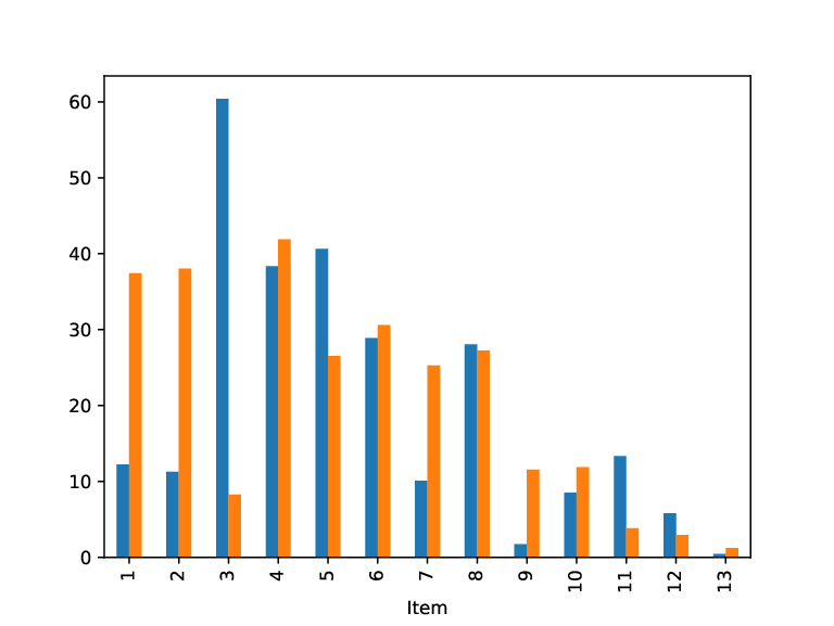
    In the figure 2 we depict two random realizations for the weights, profits and efficiencies, according to the proposed probabilistic model, Table 2 summarizes the values of the random variables for both realizations.

    Refer to caption
    (a) Weights (⁡𝐖⁡(i))i=113\big(\mathop{}\!\mathbf{W}(i)\big)_{i=1}^{13} for two random realizations.
    Refer to caption
    (b) Profits (⁡𝐏⁡(i))i=113\big(\mathop{}\!\mathbf{P}(i)\big)_{i=1}^{13} for two random realizations.
    Refer to caption
    (c) Efficiencies (⁡𝐆⁡(i))i=113\big(\mathop{}\!\mathbf{G}(i)\big)_{i=1}^{13} for two random realizations.
    Item ⁡𝐖⁡(i)\mathop{}\!\mathbf{W}(i) ⁡𝐏⁡(i)\mathop{}\!\mathbf{P}(i) ⁡𝐆⁡(i)\mathop{}\!\mathbf{G}(i)
    ii 1 2 1 2 1 2
    1 2 8 12.22 37.43 6.11 4.68
    2 2 9 11.27 38.03 5.63 4.23
    3 12 2 60.39 8.24 5.03 4.12
    4 9 11 38.35 41.9 4.26 3.81
    5 11 8 40.63 26.53 3.69 3.32
    6 8 12 28.89 30.6 3.61 2.55
    7 3 10 10.08 25.26 3.36 2.53
    8 11 11 28.07 27.23 2.55 2.48
    9 1 7 1.72 11.54 1.72 1.65
    10 6 12 8.51 11.88 1.42 0.99
    11 10 4 13.33 3.81 1.33 0.95
    12 12 5 5.81 2.93 0.48 0.59
    13 1 5 0.44 1.2 0.44 0.24
    Table 3: Numerical values for the two random realizations depicted in the graphs above.
    Figure 2: Two random realizations according to the probabilistic model introduced in Definition 5, capacity δ=12\delta=12, number of items μ=13\mu=13. Figure (a) displays the weights (⁡𝐖⁡(i))i=113(\mathop{}\!\mathbf{W}(i))_{i=1}^{13}, while figure (b) depicts the profits (⁡𝐏⁡(i))i=113(\mathop{}\!\mathbf{P}(i))_{i=1}^{13} and (c) portrays the values of the efficiencies (⁡𝐆⁡(i))i=113(\mathop{}\!\mathbf{G}(i))_{i=1}^{13}. The blue color indicates the first realization while the orange stands for the second realization. All the corresponding numerical values are summarized in the table 2.

In order to compute expected values for the Greedy Algorithm, two important random variables have to be introduced

Definition 6.

Let ⟨δ,(⁡𝐖⁡(i))i=1μ,(⁡𝐏⁡(i))i=1μ⟩\big\langle\delta,\big(\mathop{}\!\mathbf{W}(i)\big)_{i=1}^{\mu},\big(\mathop{}\!\mathbf{P}(i)\big)_{i=1}^{\mu}\big\rangle be a random instance satisfying the hypothesis 2, define

  1. (i)

    The split item random variable ⁡𝐒\mathop{}\!\mathbf{S} is the value of the index ss (introduced in Definition 1 (i)) for the random instance.

  2. (ii)

    The slack random variable is defined by

    ⁡𝐊​=𝐝𝐞𝐟​δ−∑j= 1⁡𝐒−1⁡𝐖j,\mathop{}\!\mathbf{K}\overset{\mathbf{def}}{=}\delta-\sum\limits_{j\,=\,1}^{\mathop{}\!\mathbf{S}-1}\mathop{}\!\mathbf{W}_{j}, (24)

    where ⁡𝐒\mathop{}\!\mathbf{S} is the split item random variable.

3.2 Expectations of the 0-1RKP and 0-1RLPK related variables

In this section we compute the expectations of the most important random variables related to the probabilistic model introduced in Section 3.1. We begin presenting a result which turns out to be the cornerstone of our whole construction.

Lemma 7 (Cornerstone Lemma).

Let ⁡𝐒\mathop{}\!\mathbf{S} and ⁡𝐊\mathop{}\!\mathbf{K} be the split item and the slack random variables defined above, then

ℙ(𝐊=k,𝐒=s)\displaystyle\bm{\mathbbm{P}}\big(\mathop{}\!\mathbf{K}=k,\mathop{}\!\mathbf{S}=s\big) =δ−kδs​(δ−k−1s−2),\displaystyle=\frac{\delta-k}{\delta^{s}}{\delta-k-1\choose s-2}, (25)

for s=2,…,μs=2,\ldots,\mu and k=0,…,δ−s+1k=0,\ldots,\delta-s+1.

Proof.

Observe the following equivalence of events

ℙ(𝐊=k,𝐒=s)=ℙ(δ−∑j= 1s−1𝐖(j)=k,𝐖(s)>k)=ℙ(∑j= 1s−1𝐖(j)=δ−k)ℙ(𝐖(s)>k).\begin{split}\bm{\mathbbm{P}}\big(\mathop{}\!\mathbf{K}=k,\mathop{}\!\mathbf{S}=s\big)&=\bm{\mathbbm{P}}\Big(\delta-\sum\limits_{j\,=\,1}^{s-1}\mathop{}\!\mathbf{W}(j)=k,\mathop{}\!\mathbf{W}(s)>k\Big)=\bm{\mathbbm{P}}\Big(\sum\limits_{j\,=\,1}^{s-1}\mathop{}\!\mathbf{W}(j)=\delta-k\Big)\bm{\mathbbm{P}}\Big(\mathop{}\!\mathbf{W}(s)>k\Big).\end{split}

The last equality uses the independence of the weight random variables. For the first factor we observe that the event occurs if and only if (⁡𝐖⁡(i))i=1s−1(\mathop{}\!\mathbf{W}(i))_{i=1}^{s-1} is a composition of δ−k\delta-k. According to Theorem 4 (ii) there are (δ−k−1s−2){\delta-k-1\choose s-2} of these compositions and since ⁡𝐖⁡(i)\mathop{}\!\mathbf{W}(i) are uniformly distributed over [δ][\delta], the probability for each of these compositions to occur is 1δs−1\frac{1}{\delta^{s-1}}. Next, the event [𝐖(s)>k][\mathop{}\!\mathbf{W}(s)>k] has probability δ−kδ\frac{\delta-k}{\delta} again due to the uniform distribution of the variable. Combining the previous observations, the equality (25) follows.

Finally, for the range of the variables, it is direct to see that ⁡𝐒,⁡𝐊\mathop{}\!\mathbf{S},\mathop{}\!\mathbf{K} are intertwined, then regarding ⁡𝐒\mathop{}\!\mathbf{S} as the independent and ⁡𝐊\mathop{}\!\mathbf{K} as the dependent, the first can range freely inside {2,…,δ+1}\{2,\ldots,\delta+1\} while the second only takes values within {2,…,δ−s+1}\{2,\ldots,\delta-s+1\} because ∑j= 1s−1⁡𝐖⁡(j)≥s−1\sum_{j\,=\,1}^{s-1}\mathop{}\!\mathbf{W}(j)\geq s-1. ∎

Next we compute the distribution, expectation and variance of ⁡𝐒\mathop{}\!\mathbf{S}.

Theorem 8.

Let ⁡𝐒\mathop{}\!\mathbf{S} be the splitting item random variable defined above, then its distribution and expectation are given by

ℙ⁡(⁡𝐒=s)\displaystyle\bm{\mathbbm{P}}(\mathop{}\!\mathbf{S}=s) =s−1δs(δ+1s),for all s=2,…,μ,\displaystyle=\frac{s-1}{\delta^{s}}{\delta+1\choose s},\quad\text{for all }s=2,\ldots,\mu, (26a)
𝔼⁡(⁡𝐒)\displaystyle\bm{\mathbbm{E}}(\mathop{}\!\mathbf{S}) =(1+1δ)δ,\displaystyle=\big(1+\frac{1}{\delta}\big)^{\delta}, (26b)
𝕍​𝐚𝐫​(⁡𝐒)\displaystyle\bm{\mathbbm{V}\!\mathrm{ar}}(\mathop{}\!\mathbf{S}) =(3+1δ)​(1+1δ)δ−1−(1+1δ)2​δ,\displaystyle=\big(3+\frac{1}{\delta}\big)\big(1+\frac{1}{\delta}\big)^{\delta-1}-\big(1+\frac{1}{\delta}\big)^{2\delta}, (26c)
where μ=δ+1\mu=\delta+1.
Proof.

Due to the cornerstone lemma 7 if ⁡𝐒=s\mathop{}\!\mathbf{S}=s, the slack k=δ−∑j= 1s−1⁡𝐖⁡(j)k=\delta-\sum_{j\,=\,1}^{s-1}\mathop{}\!\mathbf{W}(j) runs from 00 to δ−s+1\delta-s+1. Hence, we split the event {𝐒=s}\{\mathop{}\!\mathbf{S}=s\}, according to the range of the slack, i.e.

ℙ(𝐒=s)=∑k= 0δ−s+1ℙ(𝐊=k,𝐒=s)=∑k= 0δ−s+1δ−kδs​(δ−k−1s−2)=∑m=s−1δmδs​(m−1s−2).\begin{split}\bm{\mathbbm{P}}(\mathop{}\!\mathbf{S}=s)=\sum\limits_{k\,=\,0}^{\delta-s+1}\bm{\mathbbm{P}}(\mathop{}\!\mathbf{K}=k,\mathop{}\!\mathbf{S}=s)&=\sum\limits_{k\,=\,0}^{\delta-s+1}\frac{\delta-k}{\delta^{s}}{\delta-k-1\choose s-2}=\sum\limits_{m\,=\,s-1}^{\delta}\frac{m}{\delta^{s}}{m-1\choose s-2}.\end{split}

The first equality holds due to the cornerstone identity (25) while the second is a mere reindexing of the sum. Recalling that (m+1)​(ms−2)=(s−1)​(m+1s−1)(m+1){m\choose s-2}=(s-1){m+1\choose s-1} due to the identity (17), we have

ℙ⁡(⁡𝐒=s)=s−1δs​∑m=s−2δ(ms−1)=s−1δs​(δ+1s),\bm{\mathbbm{P}}(\mathop{}\!\mathbf{S}=s)=\frac{s-1}{\delta^{s}}\sum\limits_{m\,=\,s-2}^{\delta}{m\choose s-1}=\frac{s-1}{\delta^{s}}{\delta+1\choose s},

where the last equality holds due to the combinatorial identity (16). This proves the identity (26a). Next, in order to compute 𝔼⁡(⁡𝐒)\bm{\mathbbm{E}}(\mathop{}\!\mathbf{S}), first recall that μ=δ+1\mu=\delta+1 and get

∑s= 2δ+1s​ℙ​(⁡𝐒=s)=∑s= 2δ+1s⁡(s−1)δs​(δ+1s)=∑s= 0δ+1s⁡(s−1)δs​(δ+1s)=(δ+1)​δδ2​(1+1δ)δ−1.\begin{split}\sum\limits_{s\,=\,2}^{\delta+1}s\bm{\mathbbm{P}}(\mathop{}\!\mathbf{S}=s)=\sum\limits_{s\,=\,2}^{\delta+1}\frac{s(s-1)}{\delta^{s}}{\delta+1\choose s}&=\sum\limits_{s\,=\,0}^{\delta+1}\frac{s(s-1)}{\delta^{s}}{\delta+1\choose s}=\frac{(\delta+1)\delta}{\delta^{2}}\big(1+\frac{1}{\delta}\big)^{\delta-1}.\end{split}

Applying some basic algebraic manipulations, the identity (26b) follows. Finally, for the variance, first we compute

𝔼⁡(⁡𝐒2)=∑s= 2δ+1s2​ℙ​(⁡𝐒=s)=∑s= 2δ+1s2​s−1δs​(δ+1s)=∑s= 2δ+1s​(s−1)​(s−2)δs​(δ+1s)+2​∑s= 2δ+1s⁡(s−1)δs​(δ+1s)=(δ+1)​δ​(δ−1)δ3​(1+1δ)δ−2+2​(1+1δ)δ.\begin{split}\bm{\mathbbm{E}}(\mathop{}\!\mathbf{S}^{2})&=\sum\limits_{s\,=\,2}^{\delta+1}s^{2}\bm{\mathbbm{P}}(\mathop{}\!\mathbf{S}=s)\\ &=\sum\limits_{s\,=\,2}^{\delta+1}s^{2}\frac{s-1}{\delta^{s}}{\delta+1\choose s}\\ &=\sum\limits_{s\,=\,2}^{\delta+1}\frac{s(s-1)(s-2)}{\delta^{s}}{\delta+1\choose s}+2\sum\limits_{s\,=\,2}^{\delta+1}\frac{s(s-1)}{\delta^{s}}{\delta+1\choose s}\\ &=\frac{(\delta+1)\delta(\delta-1)}{\delta^{3}}\big(1+\frac{1}{\delta}\big)^{\delta-2}+2\big(1+\frac{1}{\delta}\big)^{\delta}.\end{split}

Here, the third equality is a convenient association of summands and the fourth equality simply uses the derivatives of the Newton’s binomial identity. Therefore,

𝕍​𝐚𝐫​(⁡𝐒)=𝔼⁡(⁡𝐒2)−𝔼2​(⁡𝐒)=(1−1δ)​(1+1δ)δ−1+2​(1+1δ)δ−(1+1δ)2​δ.\begin{split}\bm{\mathbbm{V}\!\mathrm{ar}}(\mathop{}\!\mathbf{S})=\bm{\mathbbm{E}}(\mathop{}\!\mathbf{S}^{2})-\bm{\mathbbm{E}}^{2}(\mathop{}\!\mathbf{S})&=\big(1-\frac{1}{\delta}\big)\big(1+\frac{1}{\delta}\big)^{\delta-1}+2\big(1+\frac{1}{\delta}\big)^{\delta}-\big(1+\frac{1}{\delta}\big)^{2\delta}.\end{split}

From here, the identity (26c) follows directly. ∎

Before computing the expectation of ⁡𝐙⁡G\mathop{}\!\mathbf{Z}^{\mathop{}\!\mathrm{G}} the next technical lemma is needed.

Lemma 9.

With the definitions above, the following identities hold

ℙ(𝐖(j)=w,𝐒=s)\displaystyle\bm{\mathbbm{P}}\big(\mathop{}\!\mathbf{W}(j)=w,\mathop{}\!\mathbf{S}=s\big) =1δs​(s−2)​(δ+1)+ws−1​(δ−ws−2),\displaystyle=\frac{1}{\delta^{s}}\frac{(s-2)(\delta+1)+w}{s-1}{\delta-w\choose s-2}, j=1,…,s−1\displaystyle j=1,\ldots,s-1 , (27a)
𝔼⁡(⁡𝐖⁡(j)|⁡𝐒=s)\displaystyle\bm{\mathbbm{E}}\big(\mathop{}\!\mathbf{W}(j)\big|\mathop{}\!\mathbf{S}=s\big) =δ​s+s−1s2−1,\displaystyle=\frac{\delta s+s-1}{s^{2}-1}, j=1,…,s−1.\displaystyle j=1,\ldots,s-1. (27b)
Proof.

For the first equality, observe that if ⁡𝐖⁡(j)=w\mathop{}\!\mathbf{W}(j)=w then ∑i= 1s−1⁡𝐖⁡(i)≥(s−2)+w\sum_{i\,=\,1}^{s-1}\mathop{}\!\mathbf{W}(i)\geq(s-2)+w consequently, the slack ⁡𝐊\mathop{}\!\mathbf{K} can take values only in the set {0,…,δ−(s−2)−w}\{0,\ldots,\delta-(s-2)-w\}. Hence,

ℙ(𝐖(j)=w,𝐒=s)=∑k= 0δ−(s−2)−wℙ(𝐖(j)=w,𝐊=k,𝐒=s)=∑k= 0δ−s+2−wℙ(𝐖(j)=w,∑m∈[s−1]−j𝐖(m)=δ−k−w,𝐖(s)>k)=∑k= 0δ−s+2−w1δ​1δs−2​(δ−k−w−1s−3)​δ−kδ=1δs​∑ℓ=s−3δ−w−1(ℓ+1+w)​(ℓs−3).\begin{split}\bm{\mathbbm{P}}\big(\mathop{}\!\mathbf{W}(j)=w,\mathop{}\!\mathbf{S}=s\big)=&\sum\limits_{k\,=\,0}^{\delta-(s-2)-w}\bm{\mathbbm{P}}\big(\mathop{}\!\mathbf{W}(j)=w,\mathop{}\!\mathbf{K}=k,\mathop{}\!\mathbf{S}=s\big)\\ =&\sum\limits_{k\,=\,0}^{\delta-s+2-w}\bm{\mathbbm{P}}\Big(\mathop{}\!\mathbf{W}(j)=w,\sum_{m\,\in\,[s-1]-j}\mathop{}\!\mathbf{W}(m)=\delta-k-w,\mathop{}\!\mathbf{W}(s)>k\Big)\\ =&\sum\limits_{k\,=\,0}^{\delta-s+2-w}\frac{1}{\delta}\frac{1}{\delta^{s-2}}{\delta-k-w-1\choose s-3}\frac{\delta-k}{\delta}\\ =&\frac{1}{\delta^{s}}\sum\limits_{\ell\,=\,s-3}^{\delta-w-1}(\ell+1+w){\ell\choose s-3}.\end{split}

Here, the second equality is a direct interpretation of the event ℙ(𝐖(j)=w,𝐊=k,𝐒=s)\bm{\mathbbm{P}}\big(\mathop{}\!\mathbf{W}(j)=w,\mathop{}\!\mathbf{K}=k,\mathop{}\!\mathbf{S}=s\big). The third equality is the application of the basic identity (25), while the fourth equality is the reindexing of the sum by ℓ​=𝐝𝐞𝐟​δ−k−w−1\ell\overset{\mathbf{def}}{=}\delta-k-w-1. We compute the latter sum as follows

∑ℓ=s−3δ−w−1(ℓ+1+w)​(ℓs−3)=∑ℓ=s−3δ−w−1(ℓ+1)​(ℓs−3)+w​∑ℓ=s−3δ−w−1(ℓs−3)=(s−2)​∑ℓ=s−3δ−w−1(ℓ+1s−2)+w​∑ℓ=s−3δ−w−1(ℓs−3)=(s−2)​∑m=s−2δ−w(ms−2)+w​∑ℓ=s−3δ−w−1(ℓs−3)=(s−2)​(δ−w+1s−1)+w​(δ−ws−2).\begin{split}\sum\limits_{\ell\,=\,s-3}^{\delta-w-1}(\ell+1+w){\ell\choose s-3}=&\sum\limits_{\ell\,=\,s-3}^{\delta-w-1}(\ell+1){\ell\choose s-3}+w\sum\limits_{\ell\,=\,s-3}^{\delta-w-1}{\ell\choose s-3}\\ =&(s-2)\sum\limits_{\ell\,=\,s-3}^{\delta-w-1}{\ell+1\choose s-2}+w\sum\limits_{\ell\,=\,s-3}^{\delta-w-1}{\ell\choose s-3}\\ =&(s-2)\sum\limits_{m\,=\,s-2}^{\delta-w}{m\choose s-2}+w\sum\limits_{\ell\,=\,s-3}^{\delta-w-1}{\ell\choose s-3}\\ =&(s-2){\delta-w+1\choose s-1}+w{\delta-w\choose s-2}.\end{split}

In the expression above, the second equality uses the identity (17) for shifting indexes, the third equality is a mere reindexing of the first sum and the fourth equality applies the identity (16). From here, using again the identity (δ−w+1s−1)=δ−w+1s−1​(δ−ws−2){\delta-w+1\choose s-1}=\frac{\delta-w+1}{s-1}{\delta-w\choose s-2} and performing further algebraic simplifications, the equation (27a) follows.

Next, we prove the identity (27b). Recalling the identity (20a) for conditional expectation, we get

𝔼⁡(⁡𝐖⁡(j)|⁡𝐒=s)=∑w= 1δ−(s−2)w​ℙ​(⁡𝐖⁡(j)=w|⁡𝐒=s)=1s−1δs​(δ+1s)∑w= 1δ−(s−2)wℙ(𝐖(j)=w,𝐒=s)=1s−1δs​(δ+1s)​1δs​∑w= 1δ−(s−2)(s−2)​(δ+1)​w+w2s−1​(δ−ws−2).\begin{split}\bm{\mathbbm{E}}\big(\mathop{}\!\mathbf{W}(j)\big|\mathop{}\!\mathbf{S}=s\big)=&\sum\limits_{w\,=\,1}^{\delta-(s-2)}w\bm{\mathbbm{P}}\big(\mathop{}\!\mathbf{W}(j)=w\big|\mathop{}\!\mathbf{S}=s\big)\\ =&\frac{1}{\frac{s-1}{\delta^{s}}{\delta+1\choose s}}\sum\limits_{w\,=\,1}^{\delta-(s-2)}w\bm{\mathbbm{P}}\big(\mathop{}\!\mathbf{W}(j)=w,\mathop{}\!\mathbf{S}=s\big)\\ =&\frac{1}{\frac{s-1}{\delta^{s}}{\delta+1\choose s}}\frac{1}{\delta^{s}}\sum\limits_{w\,=\,1}^{\delta-(s-2)}\frac{(s-2)(\delta+1)w+w^{2}}{s-1}{\delta-w\choose s-2}.\end{split}

Here, the second equality used the identity (19a) combined with (26a), while the third used the identity (27a). We focus on getting a closed form for the sum; by reindexing u​=𝐝𝐞𝐟​δ−wu\overset{\mathbf{def}}{=}\delta-w we get

∑w= 1δ−(s−2)(s−2)​(δ+1)​w+w2s−1​(δ−ws−2)=1s−1​∑u=s−2δ−1{(s−2)​(δ+1)​(δ−u)+(δ−u)2}​(us−2).\sum\limits_{w\,=\,1}^{\delta-(s-2)}\frac{(s-2)(\delta+1)w+w^{2}}{s-1}{\delta-w\choose s-2}=\frac{1}{s-1}\sum\limits_{u\,=\,s-2}^{\delta-1}\big\{(s-2)(\delta+1)(\delta-u)+(\delta-u)^{2}\big\}{u\choose s-2}.

Appealing to the polynomial identity

(s−2)​(δ+1)​(δ−u)+(δ−u)2=(δ+1)2​(s−1)−(s​δ+s+1)​(u+1)+(u+1)​(u+2),(s-2)(\delta+1)(\delta-u)+(\delta-u)^{2}=(\delta+1)^{2}(s-1)-(s\delta+s+1)(u+1)+(u+1)(u+2),

we have,

∑u=s−2δ−1{(δ+1)2​(s−1)−(s​δ+s+1)​(u+1)+(u+1)​(u+2)}​(us−2)=(δ+1)2​(s−1)​∑u=s−2δ−1(us−2)−(s​δ+s+1)​∑u=s−2δ−1(u+1)​(us−2)+∑u=s−2δ−1(u+1)​(u+2)​(us−2).\sum\limits_{u\,=\,s-2}^{\delta-1}\big\{(\delta+1)^{2}(s-1)-(s\delta+s+1)(u+1)+(u+1)(u+2)\big\}{u\choose s-2}\\ =(\delta+1)^{2}(s-1)\sum\limits_{u\,=\,s-2}^{\delta-1}{u\choose s-2}-(s\delta+s+1)\sum\limits_{u\,=\,s-2}^{\delta-1}(u+1){u\choose s-2}+\sum\limits_{u\,=\,s-2}^{\delta-1}(u+1)(u+2){u\choose s-2}.

Now, listing the three sums of the left hand side we have

∑u=s−2δ−1(us−2)\displaystyle\sum\limits_{u\,=\,s-2}^{\delta-1}{u\choose s-2} =(δs−1),\displaystyle={\delta\choose s-1},
∑u=s−2δ−1(u+1)​(us−2)\displaystyle\sum\limits_{u\,=\,s-2}^{\delta-1}(u+1){u\choose s-2} =(s−1)​∑u=s−2δ−1(u+1s−1)=(s−1)​∑r=s−1δ(rs−1)=(s−1)​(δ+1s),\displaystyle=(s-1)\sum\limits_{u\,=\,s-2}^{\delta-1}{u+1\choose s-1}=(s-1)\sum\limits_{r\,=\,s-1}^{\delta}{r\choose s-1}=(s-1){\delta+1\choose s},
∑u=s−2δ−1(u+2)​(u+1)​(us−2)\displaystyle\sum\limits_{u\,=\,s-2}^{\delta-1}(u+2)(u+1){u\choose s-2} =s⁡(s−1)​∑u=s−2δ−1(u+2s)=s⁡(s−1)​∑r=sδ+1(rs)=s⁡(s−1)​(δ+2s+1).\displaystyle=s(s-1)\sum\limits_{u\,=\,s-2}^{\delta-1}{u+2\choose s}=s(s-1)\sum\limits_{r\,=\,s}^{\delta+1}{r\choose s}=s(s-1){\delta+2\choose s+1}.

Combining the above with the previous gives

s−1δs​(δ+1s)​δs​𝔼​(⁡𝐖⁡(j)|⁡𝐒=s)=(δ+1)2​(δs−1)−(s​δ+s+1)​(δ+1s)+s​(δ+2s+1)=s⁡(δ+1)​(δ+1s)−(s​δ+s+1)​(δ+1s)+s​δ+2s+1​(δ+1s)=s​δ+s−1s+1​(δ+1s).\begin{split}\frac{s-1}{\delta^{s}}{\delta+1\choose s}\delta^{s}\bm{\mathbbm{E}}\big(\mathop{}\!\mathbf{W}(j)\big|\mathop{}\!\mathbf{S}=s\big)=&(\delta+1)^{2}{\delta\choose s-1}-(s\delta+s+1){\delta+1\choose s}+s{\delta+2\choose s+1}\\ =&s(\delta+1){\delta+1\choose s}-(s\delta+s+1){\delta+1\choose s}+s\frac{\delta+2}{s+1}{\delta+1\choose s}\\ =&\frac{s\delta+s-1}{s+1}{\delta+1\choose s}.\end{split}

Here, the second equality uses the identity (17) in the first and third summand, while the second equality is the mere algebraic sum of the previous line. Finally, a direct simplification of terms yields the identity (27b) and the result is complete. ∎

Theorem 10.

Let ⁡𝐒\mathop{}\!\mathbf{S} and ⁡𝐙⁡G​=𝐝𝐞𝐟​∑i= 1⁡𝐒−1⁡𝐏⁡(i)\mathop{}\!\mathbf{Z}^{\mathop{}\!\mathrm{G}}\overset{\mathbf{def}}{=}\sum\limits_{i\,=\,1}^{\mathop{}\!\mathbf{S}-1}\mathop{}\!\mathbf{P}(i) be the split item and the greedy algorithm profit random variables for the 0-1RKP (22). Then,

𝔼⁡(⁡𝐙⁡G|⁡𝐒=s)=\displaystyle\bm{\mathbbm{E}}\big(\mathop{}\!\mathbf{Z}^{\mathop{}\!\mathrm{G}}\big|\mathop{}\!\mathbf{S}=s\big)= 2​δ−s+44​δ​s+s−1s+1, for all ​s=2,…,μ,\displaystyle\frac{2\delta-s+4}{4}\frac{\delta s+s-1}{s+1},\text{ for all }s=2,\ldots,\mu, (28a)
𝔼⁡(⁡𝐙⁡G)=−(δ+1)24​δ​(1+1δ)δ−1+(2​δ+3)​(δ+2)​(δ+1)4​δ​{(1+1δ)δ−1}−(δ+2)2​{(1+1δ)δ+1−2​δ+1δ}+2​δ+52​δ​{(1+1δ)δ+2−5​δ2+7​δ+22​δ2},\displaystyle\begin{split}\bm{\mathbbm{E}}(\mathop{}\!\mathbf{Z}^{\mathop{}\!\mathrm{G}})=&-\frac{(\delta+1)^{2}}{4\delta}\big(1+\frac{1}{\delta}\big)^{\delta-1}+\frac{(2\delta+3)(\delta+2)(\delta+1)}{4\delta}\Big\{\big(1+\frac{1}{\delta}\big)^{\delta}-1\Big\}\\ &-(\delta+2)^{2}\Big\{\big(1+\frac{1}{\delta}\big)^{\delta+1}-\frac{2\delta+1}{\delta}\Big\}+\frac{2\delta+5}{2}\,\delta\Big\{\big(1+\frac{1}{\delta}\big)^{\delta+2}-\frac{5\delta^{2}+7\delta+2}{2\delta^{2}}\Big\},\end{split} (28b)

with μ=δ+1\mu=\delta+1.

Proof.

We compute the identity (28a) directly, using the definition of ⁡𝐏⁡(i)\mathop{}\!\mathbf{P}(i) introduced in Equation (21)

𝔼⁡(⁡𝐙⁡G|⁡𝐒=s)=∑j= 1s−1𝔼⁡(⁡𝐏⁡(j)|⁡𝐒=s)=∑j= 1s−1𝔼⁡(⁡𝐖⁡(j)​⁡𝐆⁡(j)|⁡𝐒=s)=∑j= 1s−1𝔼⁡(⁡𝐖⁡(j)​∑t=jμ⁡𝐓⁡(t)|⁡𝐒=s).\bm{\mathbbm{E}}\big(\mathop{}\!\mathbf{Z}^{\mathop{}\!\mathrm{G}}\big|\mathop{}\!\mathbf{S}=s\big)=\sum\limits_{j\,=\,1}^{s-1}\bm{\mathbbm{E}}\big(\mathop{}\!\mathbf{P}(j)\big|\mathop{}\!\mathbf{S}=s\big)=\sum\limits_{j\,=\,1}^{s-1}\bm{\mathbbm{E}}\big(\mathop{}\!\mathbf{W}(j)\,\mathop{}\!\mathbf{G}(j)\big|\mathop{}\!\mathbf{S}=s\big)=\sum\limits_{j\,=\,1}^{s-1}\bm{\mathbbm{E}}\Big(\mathop{}\!\mathbf{W}(j)\sum\limits_{t\,=\,j}^{\mu}\mathop{}\!\mathbf{T}(t)\big|\mathop{}\!\mathbf{S}=s\Big).

Recalling that the variables (⁡𝐖⁡(i))i=1μ\big(\mathop{}\!\mathbf{W}(i)\big)_{i=1}^{\mu} and (⁡𝐓⁡(i))i=1μ\big(\mathop{}\!\mathbf{T}(i)\big)_{i=1}^{\mu} are independent, we have

𝔼⁡(⁡𝐙⁡G|⁡𝐒=s)=∑j= 1s−1𝔼⁡(⁡𝐖⁡(j)|⁡𝐒=s)​∑t=jμ𝔼⁡(⁡𝐓⁡(t)|⁡𝐒=s)=∑j= 1s−1δ​s+s−1s2−1​μ−j+12=(s−1)​(2​μ−s+2)4​δ​s+s−1s2−1.\begin{split}\bm{\mathbbm{E}}\big(\mathop{}\!\mathbf{Z}^{\mathop{}\!\mathrm{G}}\big|\mathop{}\!\mathbf{S}=s\big)&=\sum\limits_{j\,=\,1}^{s-1}\bm{\mathbbm{E}}\big(\mathop{}\!\mathbf{W}(j)\big|\mathop{}\!\mathbf{S}=s\big)\sum\limits_{t\,=\,j}^{\mu}\bm{\mathbbm{E}}\big(\mathop{}\!\mathbf{T}(t)\big|\mathop{}\!\mathbf{S}=s\big)\\ &=\sum\limits_{j\,=\,1}^{s-1}\frac{\delta s+s-1}{s^{2}-1}\frac{\mu-j+1}{2}\\ &=\frac{(s-1)(2\mu-s+2)}{4}\frac{\delta s+s-1}{s^{2}-1}.\end{split}

Here, the second equality holds due to the identity (27b) and the distribution of the increments (⁡𝐓⁡(i))i=1μ(\mathop{}\!\mathbf{T}(i))_{i=1}^{\mu} introduced in Hypothesis 2. Simplifying the expression above, the Equation (28a) follows.

Next, we compute the expectation of ⁡𝐙⁡G\mathop{}\!\mathbf{Z}^{\mathop{}\!\mathrm{G}} conditioning on the possible values of ⁡𝐒\mathop{}\!\mathbf{S} and combining with the identities (28a), (26a); this gives

𝔼⁡(⁡𝐙⁡G)=∑s= 2δ+1𝔼⁡(⁡𝐙⁡G|⁡𝐒=s)​ℙ​(⁡𝐒=s)=∑s= 2δ+12​δ−s+44​δ​s+s−1s+1​s−1δs​(δ+1s)=14​(δ+2)​∑m= 3δ+2(m−2)​(2​δ−m+5)​((δ+1)​m−δ−2)δm−1​(δ+2m)=14​(μ+1)​∑m= 3μ+1(m−2)​(2​μ−m+3)​(μ​m−μ−1)δm−1​(μ+1m).\begin{split}\bm{\mathbbm{E}}(\mathop{}\!\mathbf{Z}^{\mathop{}\!\mathrm{G}})&=\sum\limits_{s\,=\,2}^{\delta+1}\bm{\mathbbm{E}}\big(\mathop{}\!\mathbf{Z}^{\mathop{}\!\mathrm{G}}\big|\mathop{}\!\mathbf{S}=s\big)\bm{\mathbbm{P}}\big(\mathop{}\!\mathbf{S}=s\big)\\ &=\sum\limits_{s\,=\,2}^{\delta+1}\frac{2\delta-s+4}{4}\frac{\delta s+s-1}{s+1}\frac{s-1}{\delta^{s}}{\delta+1\choose s}\\ &=\frac{1}{4(\delta+2)}\sum\limits_{m\,=\,3}^{\delta+2}\frac{(m-2)(2\delta-m+5)\big((\delta+1)m-\delta-2\big)}{\delta^{m-1}}{\delta+2\choose m}\\ &=\frac{1}{4(\mu+1)}\sum\limits_{m\,=\,3}^{\mu+1}\frac{(m-2)(2\mu-m+3)\big(\mu m-\mu-1\big)}{\delta^{m-1}}{\mu+1\choose m}.\end{split}

The third equality in the expression above is a convenient reindexing of the sum, while the last equality follows from the substitution μ=δ+1\mu=\delta+1. Next, consider the polynomial identity

(m−2)​(2​μ−m+3)​(μ​m−μ−1)=−μ​m​(m−1)​(m−2)+(2​μ+1)​(μ+1)​m​(m−1)−4​(μ+1)2​m+(4​μ+6)​(μ+1),(m-2)(2\mu-m+3)(\mu m-\mu-1)=\\ -\mu m(m-1)(m-2)+(2\mu+1)(\mu+1)m(m-1)-4(\mu+1)^{2}m+(4\mu+6)(\mu+1),

and combine it with the expression above. We get

𝔼⁡(⁡𝐙⁡G)=−14​δ2μμ+1∑m= 3μ+1m​(m−1)​(m−2)δm−3(μ+1m)+2​μ+14​δ∑m= 3μ+1m⁡(m−1)δm−2(μ+1m)−(μ+1)∑m= 3μ+1mδm−1(μ+1m)+δ4​μ+64∑m= 3μ+11δm(μ+1m)=−14​δ2​μμ+1​(μ+1)​μ​(μ−1)​(1+1δ)μ−2+2​μ+14​δ​{(μ+1)​μ​(1+1δ)μ−1−(μ+1)​μ}−(μ+1)​{(μ+1)​(1+1δ)μ−(μ+1)−μ⁡(μ+1)δ}+δ​4​μ+64​{(1+1δ)μ+1−1−μ+1δ−(μ+1)​μ2​δ2}.\begin{split}\bm{\mathbbm{E}}(\mathop{}\!\mathbf{Z}^{\mathop{}\!\mathrm{G}})=&-\frac{1}{4\delta^{2}}\frac{\mu}{\mu+1}\sum\limits_{m\,=\,3}^{\mu+1}\frac{m(m-1)(m-2)}{\delta^{m-3}}{\mu+1\choose m}+\frac{2\mu+1}{4\delta}\sum\limits_{m\,=\,3}^{\mu+1}\frac{m(m-1)}{\delta^{m-2}}{\mu+1\choose m}\\ &-(\mu+1)\sum\limits_{m\,=\,3}^{\mu+1}\frac{m}{\delta^{m-1}}{\mu+1\choose m}+\delta\frac{4\mu+6}{4}\sum\limits_{m\,=\,3}^{\mu+1}\frac{1}{\delta^{m}}{\mu+1\choose m}\\ =&-\frac{1}{4\delta^{2}}\frac{\mu}{\mu+1}(\mu+1)\mu(\mu-1)\big(1+\frac{1}{\delta}\big)^{\mu-2}+\frac{2\mu+1}{4\delta}\Big\{(\mu+1)\mu\big(1+\frac{1}{\delta}\big)^{\mu-1}-(\mu+1)\mu\Big\}\\ &-(\mu+1)\Big\{(\mu+1)\big(1+\frac{1}{\delta}\big)^{\mu}-(\mu+1)-\frac{\mu(\mu+1)}{\delta}\Big\}\\ &+\delta\frac{4\mu+6}{4}\Big\{\big(1+\frac{1}{\delta}\big)^{\mu+1}-1-\frac{\mu+1}{\delta}-\frac{(\mu+1)\mu}{2\delta^{2}}\Big\}.\end{split}

Simplifying the latter and replacing back δ=μ−1\delta=\mu-1, the equality (28b) follows. ∎

Next we find the distribution, conditional expectation with respect to ⁡𝐒\mathop{}\!\mathbf{S} and expectation for the slack ⁡𝐊\mathop{}\!\mathbf{K}.

Theorem 11.

The slack random variable ⁡𝐊\mathop{}\!\mathbf{K}, introduced in Definition 6 (ii), satisfies

ℙ⁡(⁡𝐊=k)=\displaystyle\bm{\mathbbm{P}}\big(\mathop{}\!\mathbf{K}=k\big)= δ−kδ2​(1+1δ)δ−k−1, for all ​k=0,…,δ.\displaystyle\frac{\delta-k}{\delta^{2}}\big(1+\frac{1}{\delta}\big)^{\delta-k-1},\text{ for all }k=0,\ldots,\delta. (29a)
𝔼⁡(⁡𝐊|⁡𝐒=s)=\displaystyle\bm{\mathbbm{E}}\big(\mathop{}\!\mathbf{K}\big|\mathop{}\!\mathbf{S}=s\big)= δ+1−ss+1, for all ​s=2,…,μ.\displaystyle\frac{\delta+1-s}{s+1}\,,\text{ for all }s=2,\ldots,\mu. (29b)
𝔼⁡(⁡𝐊)=−(δ+1)δ​{(1+1δ)δ−1}+(δ+3)​{(1+1δ)δ+1−2​δ+1δ}−2​δ​{(1+1δ)δ+2−5​δ2+7​δ+22​δ2}.\displaystyle\begin{split}\bm{\mathbbm{E}}\big(\mathop{}\!\mathbf{K}\big)=&-\frac{(\delta+1)}{\delta}\Big\{\big(1+\frac{1}{\delta}\big)^{\delta}-1\Big\}+(\delta+3)\Big\{\big(1+\frac{1}{\delta}\big)^{\delta+1}-\frac{2\delta+1}{\delta}\Big\}\\ &-2\delta\Big\{\big(1+\frac{1}{\delta}\big)^{\delta+2}-\frac{5\delta^{2}+7\delta+2}{2\delta^{2}}\Big\}.\end{split} (29c)
Proof.

Revisiting the cornerstone lemma 7, observe that fixing ⁡𝐊=k\mathop{}\!\mathbf{K}=k, the range of the split index ss is {2,…,δ−k+1}\{2,\ldots,\delta-k+1\}. Hence,

ℙ(𝐊=k)=∑s= 2δ−k+1ℙ(𝐊=k,𝐒=s)=∑s= 2δ−k+1s−1δs​(δ−ks−1)=1δ2​∑j= 1δ−kjδj−1​(δ−kj).\begin{split}\bm{\mathbbm{P}}(\mathop{}\!\mathbf{K}=k)=\sum\limits_{s\,=\,2}^{\delta-k+1}\bm{\mathbbm{P}}(\mathop{}\!\mathbf{K}=k,\mathop{}\!\mathbf{S}=s)=&\sum\limits_{s\,=\,2}^{\delta-k+1}\frac{s-1}{\delta^{s}}{\delta-k\choose s-1}=\frac{1}{\delta^{2}}\sum\limits_{j\,=\,1}^{\delta-k}\frac{j}{\delta^{j-1}}{\delta-k\choose j}.\end{split}

Here, the second equality holds due to the cornerstone identity (25), the third equality is a convenient reindexing and association of terms. Then, applying the first derivative of the Newton’s binomial expansion, the identity (29a) follows.

Next, we show the equality (29b). From the cornerstone lemma 7 observe that if ⁡𝐒=s\mathop{}\!\mathbf{S}=s the range of the slack ⁡𝐊\mathop{}\!\mathbf{K} is {0,…,δ−s+1}\{0,\ldots,\delta-s+1\}. Hence, recalling the conditional expectation identity (20a) we get

𝔼(𝐊|𝐒=s)=∑k= 0δ−s+1kℙ(𝐊=k|𝐒=s)=1ℙ⁡(⁡𝐒=s)∑k= 0δ−s+1kℙ(𝐊=k,𝐒=s).\bm{\mathbbm{E}}\big(\mathop{}\!\mathbf{K}\big|\mathop{}\!\mathbf{S}=s\big)=\sum\limits_{k\,=\,0}^{\delta-s+1}k\bm{\mathbbm{P}}\big(\mathop{}\!\mathbf{K}=k\big|\mathop{}\!\mathbf{S}=s)=\frac{1}{\bm{\mathbbm{P}}(\mathop{}\!\mathbf{S}=s)}\sum\limits_{k\,=\,0}^{\delta-s+1}k\bm{\mathbbm{P}}\big(\mathop{}\!\mathbf{K}=k,\mathop{}\!\mathbf{S}=s).

Now, appealing to the basic identiy (25), we have

𝔼⁡(⁡𝐊|⁡𝐒=s)=1ℙ⁡(⁡𝐒=s)​1δs​∑k= 0δ−s+1(δ−k)​k​(δ−k−1s−2)=1ℙ⁡(⁡𝐒=s)​1δs​∑j=s−1δj⁡(δ−j)​(j−1s−2)=1ℙ⁡(⁡𝐒=s)​δ+1δs​∑j=s−1δj​(j−1s−2)−1ℙ⁡(⁡𝐒=s)​1δs​∑j=s−1δ(j+1)​j​(j−1s−2).\begin{split}\bm{\mathbbm{E}}\big(\mathop{}\!\mathbf{K}\big|\mathop{}\!\mathbf{S}=s\big)&=\frac{1}{\bm{\mathbbm{P}}(\mathop{}\!\mathbf{S}=s)}\frac{1}{\delta^{s}}\sum\limits_{k\,=\,0}^{\delta-s+1}(\delta-k)k{\delta-k-1\choose s-2}\\ &=\frac{1}{\bm{\mathbbm{P}}(\mathop{}\!\mathbf{S}=s)}\frac{1}{\delta^{s}}\sum\limits_{j\,=\,s-1}^{\delta}j(\delta-j){j-1\choose s-2}\\ &=\frac{1}{\bm{\mathbbm{P}}(\mathop{}\!\mathbf{S}=s)}\frac{\delta+1}{\delta^{s}}\sum\limits_{j\,=\,s-1}^{\delta}j{j-1\choose s-2}-\frac{1}{\bm{\mathbbm{P}}(\mathop{}\!\mathbf{S}=s)}\frac{1}{\delta^{s}}\sum\limits_{j\,=\,s-1}^{\delta}(j+1)j{j-1\choose s-2}.\end{split}

Here, the second equality follows from reindexing j=δ−kj=\delta-k, while the third equality is a mere convenient association of summands. Next from the identity (17), we get the equalities js−1​(j−1s−2)=(js−1)\frac{j}{s-1}{j-1\choose s-2}={j\choose s-1}, j⁡(j+1)s⁡(s−1)​(j−1s−2)=(j+1s)\frac{j(j+1)}{s(s-1)}{j-1\choose s-2}={j+1\choose s} for the first and second summands respectively. From here, proceeding as in the proofs of Lemma 9 and Theorem 10, the identity (29b) follows.

Finally, we pursue a closed form for 𝔼⁡(⁡𝐊)\bm{\mathbbm{E}}(\mathop{}\!\mathbf{K}); to that end we apply the identity (20c) and get

𝔼⁡(⁡𝐊)=∑s= 2δ+1𝔼⁡(⁡𝐊|⁡𝐒=s)​ℙ​(⁡𝐒=s)=∑s= 2δ+1δ+1−ss+1​s−1δs​(δ+1s)=1δ+2​∑s= 2δ+1(δ+1−s)​(s−1)δs​(δ+2s+1)=1δ+2​∑j= 3δ+2(δ+2−j)​(j−2)δj−1​(δ+2j).\begin{split}\bm{\mathbbm{E}}\big(\mathop{}\!\mathbf{K}\big)=&\sum\limits_{s\,=\,2}^{\delta+1}\bm{\mathbbm{E}}\big(\mathop{}\!\mathbf{K}\big|\mathop{}\!\mathbf{S}=s\big)\bm{\mathbbm{P}}\big(\mathop{}\!\mathbf{S}=s\big)=\sum\limits_{s\,=\,2}^{\delta+1}\frac{\delta+1-s}{s+1}\frac{s-1}{\delta^{s}}{\delta+1\choose s}\\ =&\frac{1}{\delta+2}\sum\limits_{s\,=\,2}^{\delta+1}\frac{(\delta+1-s)(s-1)}{\delta^{s}}{\delta+2\choose s+1}=\frac{1}{\delta+2}\sum\limits_{j\,=\,3}^{\delta+2}\frac{(\delta+2-j)(j-2)}{\delta^{j-1}}{\delta+2\choose j}.\end{split}

Here, the second equality follows by replacing the equations (29b) and (26a). The third equality uses the identity (17) and the fourth equality follows from the convenient reindexing j=s+1j=s+1. Next, we replace the polynomial identity

(δ+2−j)​(j−2)=−j⁡(j+1)+(δ+3)​j−2​(δ+2),(\delta+2-j)(j-2)=-j(j+1)+(\delta+3)j-2(\delta+2),

in the expression above and get

(δ+2)​𝔼​(⁡𝐊)=−1δ∑j= 3δ+2j⁡(j−1)δj−2(δ+2j)+(δ+3)∑j= 3δ+2jδj−1(δ+2j)−2δ(δ+2)∑j= 3δ+21δj(δ+2j)=−1δ​{(δ+2)​(δ+1)​(1+1δ)δ−(δ+2)​(δ+1)}+(δ+3)​{(δ+2)​(1+1δ)δ+1−(δ+2)−(δ+2)​(δ+1)δ}−2​δ​(δ+2)​{(1+1δ)δ+2−1−δ+2δ−(δ+2)​(δ+1)2​δ2}.\begin{split}(\delta+2)\bm{\mathbbm{E}}\big(\mathop{}\!\mathbf{K}\big)=&-\frac{1}{\delta}\sum\limits_{j\,=\,3}^{\delta+2}\frac{j(j-1)}{\delta^{j-2}}{\delta+2\choose j}+(\delta+3)\sum\limits_{j\,=\,3}^{\delta+2}\frac{j}{\delta^{j-1}}{\delta+2\choose j}-2\delta(\delta+2)\sum\limits_{j\,=\,3}^{\delta+2}\frac{1}{\delta^{j}}{\delta+2\choose j}\\ =&-\frac{1}{\delta}\Big\{(\delta+2)(\delta+1)\big(1+\frac{1}{\delta}\big)^{\delta}-(\delta+2)(\delta+1)\Big\}\\ &+(\delta+3)\Big\{(\delta+2)\big(1+\frac{1}{\delta}\big)^{\delta+1}-(\delta+2)-\frac{(\delta+2)(\delta+1)}{\delta}\Big\}\\ &-2\delta(\delta+2)\Big\{\big(1+\frac{1}{\delta}\big)^{\delta+2}-1-\frac{\delta+2}{\delta}-\frac{(\delta+2)(\delta+1)}{2\delta^{2}}\Big\}.\end{split}

Here, the second equality uses the Newton’s binomial expansion, together with its first and second derivatives. Finally, simplifying the latter expression the equality (29c) follows. ∎

Theorem 12.

Let ⁡𝐙⁡LP\mathop{}\!\mathbf{Z}^{\mathop{}\!\mathrm{LP}} be the optimal profit value given by the linear relaxation of the 0-1RKP (22). Then, its expected value is given by

𝔼⁡(⁡𝐙⁡LP)=𝔼⁡(⁡𝐙⁡G)+δ+12​δ​(1+1δ)δ−1−(δ+2)​(δ+1)δ​{(1+1δ)δ−1}+(δ+5)​(δ+2)2​{(1+1δ)δ−1−2​δ+1δ}−(δ+3)​δ​{(1+1δ)δ+2−5​δ2+7​δ+22​δ2}=−(δ+1)​(δ−1)4​δ​(1+1δ)δ−1+(2​δ−1)​(δ+2)​(δ+1)4​δ​{(1+1δ)δ−1}−(δ+2)​(δ−1)2​{(1+1δ)δ+1−2​δ+1δ}−12​δ​{(1+1δ)δ+2−5​δ2+7​δ+22​δ2}.\begin{split}\bm{\mathbbm{E}}(\mathop{}\!\mathbf{Z}^{\mathop{}\!\mathrm{LP}})=&\bm{\mathbbm{E}}(\mathop{}\!\mathbf{Z}^{\mathop{}\!\mathrm{G}})+\frac{\delta+1}{2\delta}\big(1+\frac{1}{\delta}\big)^{\delta-1}-\frac{(\delta+2)(\delta+1)}{\delta}\Big\{(1+\frac{1}{\delta}\big)^{\delta}-1\Big\}\\ &+\frac{(\delta+5)(\delta+2)}{2}\Big\{\big(1+\frac{1}{\delta}\big)^{\delta-1}-\frac{2\delta+1}{\delta}\Big\}-(\delta+3)\delta\Big\{\big(1+\frac{1}{\delta}\big)^{\delta+2}-\frac{5\delta^{2}+7\delta+2}{2\delta^{2}}\Big\}\\ =&-\frac{(\delta+1)(\delta-1)}{4\delta}\big(1+\frac{1}{\delta}\big)^{\delta-1}+\frac{(2\delta-1)(\delta+2)(\delta+1)}{4\delta}\Big\{\big(1+\frac{1}{\delta}\big)^{\delta}-1\Big\}\\ &-\frac{(\delta+2)(\delta-1)}{2}\Big\{\big(1+\frac{1}{\delta}\big)^{\delta+1}-\frac{2\delta+1}{\delta}\Big\}-\frac{1}{2}\,\delta\Big\{\big(1+\frac{1}{\delta}\big)^{\delta+2}-\frac{5\delta^{2}+7\delta+2}{2\delta^{2}}\Big\}.\end{split} (30)

Here, ⁡𝐙⁡G\mathop{}\!\mathbf{Z}^{\mathop{}\!\mathrm{G}} is the profit of the solution furnished by the greedy algorithm, whose expectation 𝔼⁡(⁡𝐙⁡G)\bm{\mathbbm{E}}(\mathop{}\!\mathbf{Z}^{\mathop{}\!\mathrm{G}}) is given by the identity (28b).

Proof.

Due to Theorem 1 (ii), equation (9b), we know that

⁡𝐙⁡LP=∑j= 1⁡𝐒−1⁡𝐏⁡(j)+1⁡𝐖⁡(⁡𝐒)​(δ−∑j= 1⁡𝐒−1⁡𝐖⁡(j))​⁡𝐏⁡(⁡𝐒)=⁡𝐙⁡G+⁡𝐊⋅⁡𝐆⁡(⁡𝐒)=⁡𝐙⁡G+⁡𝐊​∑ℓ=⁡𝐒μ⁡𝐓⁡(ℓ).\mathop{}\!\mathbf{Z}^{\mathop{}\!\mathrm{LP}}=\sum\limits_{j\,=\,1}^{\mathop{}\!\mathbf{S}-1}\mathop{}\!\mathbf{P}(j)+\dfrac{1}{\mathop{}\!\mathbf{W}(\mathop{}\!\mathbf{S})}\Big(\delta-\sum\limits_{j\,=\,1}^{\mathop{}\!\mathbf{S}-1}\mathop{}\!\mathbf{W}(j)\Big)\mathop{}\!\mathbf{P}(\mathop{}\!\mathbf{S})=\mathop{}\!\mathbf{Z}^{\mathop{}\!\mathrm{G}}+\mathop{}\!\mathbf{K}\cdot\mathop{}\!\mathbf{G}(\mathop{}\!\mathbf{S})=\mathop{}\!\mathbf{Z}^{\mathop{}\!\mathrm{G}}+\mathop{}\!\mathbf{K}\sum\limits_{\ell\,=\,\mathop{}\!\mathbf{S}}^{\mu}\mathop{}\!\mathbf{T}(\ell). (31)

Hence, conditioning on ⁡𝐒\mathop{}\!\mathbf{S} through its range and recalling the equalities (29b), (26a), we have

𝔼⁡(⁡𝐙⁡LP)=𝔼⁡(⁡𝐙⁡G)+∑s= 2μ𝔼⁡(⁡𝐊​∑ℓ=⁡𝐒μ⁡𝐓⁡(ℓ)|⁡𝐒=s)​ℙ​(⁡𝐒=s)=𝔼⁡(⁡𝐙⁡G)+∑s= 2μ𝔼⁡(⁡𝐊|⁡𝐒=s)​𝔼​(∑ℓ=⁡𝐒μ⁡𝐓⁡(ℓ)|⁡𝐒=s)​ℙ​(⁡𝐒=s)=𝔼⁡(⁡𝐙⁡G)+∑s= 2μδ+1−ss+1​μ−s+12​s−1δs​(δ+1s)=𝔼⁡(⁡𝐙⁡G)+12​1δ+2​∑s= 2μ(μ−s)​(μ+1−s)​(s−1)δs​(δ+2s+1)=𝔼⁡(⁡𝐙⁡G)+12​1μ+1​∑m= 3μ+1(μ+1−m)​(μ+2−m)​(m−2)δm−1​(μ+1m)⏟=𝐝𝐞𝐟​Σ\begin{split}\bm{\mathbbm{E}}(\mathop{}\!\mathbf{Z}^{\mathop{}\!\mathrm{LP}})=&\bm{\mathbbm{E}}(\mathop{}\!\mathbf{Z}^{\mathop{}\!\mathrm{G}})+\sum_{s\,=\,2}^{\mu}\bm{\mathbbm{E}}\Big(\mathop{}\!\mathbf{K}\sum\limits_{\ell\,=\,\mathop{}\!\mathbf{S}}^{\mu}\mathop{}\!\mathbf{T}(\ell)\Big|\mathop{}\!\mathbf{S}=s\Big)\bm{\mathbbm{P}}(\mathop{}\!\mathbf{S}=s)\\ =&\bm{\mathbbm{E}}(\mathop{}\!\mathbf{Z}^{\mathop{}\!\mathrm{G}})+\sum_{s\,=\,2}^{\mu}\bm{\mathbbm{E}}\big(\mathop{}\!\mathbf{K}\big|\mathop{}\!\mathbf{S}=s\big)\bm{\mathbbm{E}}\Big(\sum\limits_{\ell\,=\,\mathop{}\!\mathbf{S}}^{\mu}\mathop{}\!\mathbf{T}(\ell)\Big|\mathop{}\!\mathbf{S}=s\Big)\bm{\mathbbm{P}}(\mathop{}\!\mathbf{S}=s)\\ =&\bm{\mathbbm{E}}(\mathop{}\!\mathbf{Z}^{\mathop{}\!\mathrm{G}})+\sum_{s\,=\,2}^{\mu}\frac{\delta+1-s}{s+1}\frac{\mu-s+1}{2}\frac{s-1}{\delta^{s}}{\delta+1\choose s}\\ =&\bm{\mathbbm{E}}(\mathop{}\!\mathbf{Z}^{\mathop{}\!\mathrm{G}})+\frac{1}{2}\frac{1}{\delta+2}\sum_{s\,=\,2}^{\mu}\frac{(\mu-s)(\mu+1-s)(s-1)}{\delta^{s}}{\delta+2\choose s+1}\\ =&\bm{\mathbbm{E}}(\mathop{}\!\mathbf{Z}^{\mathop{}\!\mathrm{G}})+\underbrace{\frac{1}{2}\frac{1}{\mu+1}\sum_{m\,=\,3}^{\mu+1}\frac{(\mu+1-m)(\mu+2-m)(m-2)}{\delta^{m-1}}{\mu+1\choose m}}_{\overset{\mathbf{def}}{=}\Sigma}\end{split}

In the expression above, the fourth equality uses the identities μ=δ+1\mu=\delta+1 and (17). The fifth equality follows from reindexing m=s+1m=s+1; here we also denote the second summand term by Σ\Sigma. Next, we focus on deriving a closed form for Σ\Sigma, to that end, we appeal to the polynomial identity

(μ+1−m)​(μ+2−m)​(m−2)=m⁡(m−1)​(m−2)−2​(μ+1)​m​(m−1)+(μ+4)​(μ+1)​m−2​(μ+2)​(μ+1).(\mu+1-m)(\mu+2-m)(m-2)\\ =m(m-1)(m-2)-2(\mu+1)m(m-1)+(\mu+4)(\mu+1)m-2(\mu+2)(\mu+1).

Replacing the latter in the second summand Σ\Sigma, it transforms in

Σ≡12​δ2​1μ+1​∑m= 3μ+1m​(m−1)​(m−2)δm−3​(μ+1m)−1δ​∑m= 3μ+1m⁡(m−1)δm−2​(μ+1m)+μ+42∑m= 3μ+1mδm−1(μ+1m)−δ(μ+2)∑m= 3μ+11δm(μ+1m)=μ2​δ​(1+1δ)μ−2−(μ+1)​μδ​{(1+1δ)μ−1−1}+(μ+4)​(μ+1)2​{(1+1δ)μ−1−μδ}−δ⁡(μ+2)​{(1+1δ)μ+1−1−μ+1δ−(μ+1)​μ2​δ2}=δ+12​δ​(1+1δ)δ−1−(δ+2)​(δ+1)δ​{(1+1δ)δ−1}+(δ+5)​(δ+2)2​{(1+1δ)δ−1−1−δ+1δ}−δ⁡(δ+3)​{(1+1δ)δ+2−1−δ+2δ−(δ+2)​(δ+1)2​δ2}.\begin{split}\Sigma\equiv&\frac{1}{2\delta^{2}}\frac{1}{\mu+1}\sum_{m\,=\,3}^{\mu+1}\frac{m(m-1)(m-2)}{\delta^{m-3}}{\mu+1\choose m}-\frac{1}{\delta}\sum_{m\,=\,3}^{\mu+1}\frac{m(m-1)}{\delta^{m-2}}{\mu+1\choose m}\\ &+\frac{\mu+4}{2}\sum_{m\,=\,3}^{\mu+1}\frac{m}{\delta^{m-1}}{\mu+1\choose m}-\delta(\mu+2)\sum_{m\,=\,3}^{\mu+1}\frac{1}{\delta^{m}}{\mu+1\choose m}\\ =&\frac{\mu}{2\delta}\big(1+\frac{1}{\delta}\big)^{\mu-2}-\frac{(\mu+1)\mu}{\delta}\Big\{(1+\frac{1}{\delta}\big)^{\mu-1}-1\Big\}+\frac{(\mu+4)(\mu+1)}{2}\Big\{\big(1+\frac{1}{\delta}\big)^{\mu}-1-\frac{\mu}{\delta}\Big\}\\ &-\delta(\mu+2)\Big\{\big(1+\frac{1}{\delta}\big)^{\mu+1}-1-\frac{\mu+1}{\delta}-\frac{(\mu+1)\mu}{2\delta^{2}}\Big\}\\ =&\frac{\delta+1}{2\delta}\big(1+\frac{1}{\delta}\big)^{\delta-1}-\frac{(\delta+2)(\delta+1)}{\delta}\Big\{(1+\frac{1}{\delta}\big)^{\delta}-1\Big\}+\frac{(\delta+5)(\delta+2)}{2}\Big\{\big(1+\frac{1}{\delta}\big)^{\delta-1}-1-\frac{\delta+1}{\delta}\Big\}\\ &-\delta(\delta+3)\Big\{\big(1+\frac{1}{\delta}\big)^{\delta+2}-1-\frac{\delta+2}{\delta}-\frac{(\delta+2)(\delta+1)}{2\delta^{2}}\Big\}.\end{split}

Here, the second equality was attained using Newton’s binomial identity, together with its first three derivatives. The last equality was attained by replacing δ=μ−1\delta=\mu-1. Performing further simplifications we get the first equality in the identity (30) and replacing (28b) in it, we obtain the second equality. ∎

Definition 7.

Define the post-greedy profit random variable, associated with the 0-1RLPK, as

⁡𝐘⁡LP​=𝐝𝐞𝐟​⁡𝐊⋅⁡𝐆⁡(⁡𝐒).\mathop{}\!\mathbf{Y}^{\mathop{}\!\mathrm{LP}}\overset{\mathbf{def}}{=}\mathop{}\!\mathbf{K}\cdot\mathop{}\!\mathbf{G}(\mathop{}\!\mathbf{S}). (32)
Theorem 13 (Asymptotic Relations).

Let ⁡𝐒,⁡𝐊,⁡𝐙⁡G\mathop{}\!\mathbf{S},\mathop{}\!\mathbf{K},\mathop{}\!\mathbf{Z}^{\mathop{}\!\mathrm{G}} and ⁡𝐙⁡LP\mathop{}\!\mathbf{Z}^{\mathop{}\!\mathrm{LP}} be the random variables defined so far, then the following limits hold

limδ→∞𝔼⁡(⁡𝐒)\displaystyle\lim\limits_{\delta\,\rightarrow\,\infty}\bm{\mathbbm{E}}\big(\mathop{}\!\mathbf{S}\big) =e,\displaystyle=e, (33a)
limδ→∞𝕍​𝐚𝐫​(⁡𝐒)\displaystyle\lim\limits_{\delta\,\rightarrow\,\infty}\bm{\mathbbm{V}\!\mathrm{ar}}\big(\mathop{}\!\mathbf{S}\big) =e⁡(3​e−e),\displaystyle=e\big(3e-e\big), (33b)
limδ→∞𝔼⁡(⁡𝐊)δ\displaystyle\lim\limits_{\delta\,\rightarrow\,\infty}\frac{\bm{\mathbbm{E}}\big(\mathop{}\!\mathbf{K}\big)}{\delta} =3−e,\displaystyle=3-e, (33c)
limδ→∞𝔼⁡(⁡𝐙⁡G)+δ−𝔼⁡(⁡𝐒)+12​𝔼​(⁡𝐊)𝔼⁡(⁡𝐙⁡LP)\displaystyle\lim\limits_{\delta\,\rightarrow\,\infty}\frac{\bm{\mathbbm{E}}(\mathop{}\!\mathbf{Z}^{\mathop{}\!\mathrm{G}})+\dfrac{\delta-\bm{\mathbbm{E}}(\mathop{}\!\mathbf{S})+1}{2}\bm{\mathbbm{E}}(\mathop{}\!\mathbf{K})}{\bm{\mathbbm{E}}\big(\mathop{}\!\mathbf{Z}^{\mathop{}\!\mathrm{LP}}\big)} =1,\displaystyle=1, (33d)
limδ→∞𝔼⁡(⁡𝐙⁡G)𝔼⁡(⁡𝐙⁡LP)\displaystyle\lim\limits_{\delta\,\rightarrow\,\infty}\frac{\bm{\mathbbm{E}}\big(\mathop{}\!\mathbf{Z}^{\mathop{}\!\mathrm{G}}\big)}{\bm{\mathbbm{E}}\big(\mathop{}\!\mathbf{Z}^{\mathop{}\!\mathrm{LP}}\big)} =e−2,\displaystyle=e-2, (33e)
limδ→∞δ−𝔼⁡(⁡𝐒)+12​𝔼​(⁡𝐊)𝔼⁡(⁡𝐙⁡LP)\displaystyle\lim\limits_{\delta\,\rightarrow\,\infty}\frac{\dfrac{\delta-\bm{\mathbbm{E}}(\mathop{}\!\mathbf{S})+1}{2}\bm{\mathbbm{E}}(\mathop{}\!\mathbf{K})}{\bm{\mathbbm{E}}\big(\mathop{}\!\mathbf{Z}^{\mathop{}\!\mathrm{LP}}\big)} =3−e.\displaystyle=3-e. (33f)
Sketch of the proof.

An elementary calculation of limits on the corresponding closed formulas developed above gives all the desired results. ∎

Remark 7.

Observe that if we approximate 𝔼⁡(⁡𝐊​∑t=⁡𝐒μ⁡𝐓⁡(t))\bm{\mathbbm{E}}(\mathop{}\!\mathbf{K}\sum_{t\,=\,\mathop{}\!\mathbf{S}}^{\mu}\mathop{}\!\mathbf{T}(t)) with δ−𝔼⁡(⁡𝐒)+12​𝔼​(⁡𝐊)\frac{\delta-\bm{\mathbbm{E}}(\mathop{}\!\mathbf{S})+1}{2}\bm{\mathbbm{E}}(\mathop{}\!\mathbf{K}) then, the expression 𝔼⁡(⁡𝐙⁡G)+δ−𝔼⁡(⁡𝐒)+12​𝔼​(⁡𝐊)\bm{\mathbbm{E}}(\mathop{}\!\mathbf{Z}^{\mathop{}\!\mathrm{G}})+\frac{\delta-\bm{\mathbbm{E}}(\mathop{}\!\mathbf{S})+1}{2}\bm{\mathbbm{E}}(\mathop{}\!\mathbf{K}) is an approximation of 𝔼⁡(⁡𝐙⁡LP)\bm{\mathbbm{E}}(\mathop{}\!\mathbf{Z}^{\mathop{}\!\mathrm{LP}}) as the equation (31) shows. Hence, the statement (33d) proves that this is a good approximation.

3.3 The expected performance of the eligible-first algorithm

We close this section presenting the computation of the eligible-first algorithm expectation 𝔼⁡(⁡𝐙⁡eF)\bm{\mathbbm{E}}(\mathop{}\!\mathbf{Z}^{\mathop{}\!\mathrm{eF}}). Given that the proofs are remarkably similar to those presented in the previous section, we only present sketches of them with some important highlights.

Definition 8.

Let ⁡𝐊\mathop{}\!\mathbf{K} and ⁡𝐒\mathop{}\!\mathbf{S} be the random variables introduced in Definition 6

  1. (i)

    Let EE be the set defined in (7a). We say an item i∈[μ]i\in[\mu] is eligible-first eF if it is the least element of the set EE i.e., if it is the first eligible item, once the greedy algorithm has stopped packing items.

  2. (ii)

    For the eligible-first algorithm, we define its corresponding post-greedy profit random variable as follows

    ⁡𝐘⁡eF={⁡𝐏⁡(i)i​ is ​⁡eF,0,E=∅.\displaystyle\mathop{}\!\mathbf{Y}^{\mathop{}\!\mathrm{eF}}=\begin{cases}\mathop{}\!\mathbf{P}(i)&i\text{ is }\mathop{}\!\mathrm{eF},\\ 0,&E=\emptyset.\end{cases} (34)
Lemma 14.

With the definitions above we have

ℙ(i is eF,𝐊=k,𝐒=s)\displaystyle\bm{\mathbbm{P}}\big(i\text{ is }\mathop{}\!\mathrm{eF},\mathop{}\!\mathbf{K}=k,\mathop{}\!\mathbf{S}=s\big) =δ−kδs+1​k​(1−kδ)i−s−1​(δ−k−1s−2),\displaystyle=\frac{\delta-k}{\delta^{s+1}}k\big(1-\frac{k}{\delta}\big)^{i-s-1}{\delta-k-1\choose s-2}, (35a)
for i=s+1,…,μi=s+1,\ldots,\mu, k=0,…,δ−s−1k=0,\ldots,\delta-s-1, s=2,…,μs=2,\ldots,\mu.
𝔼(𝐘⁡eF|𝐊=k,𝐒=s)=k4​(δ−s+1)​{1−(1−kδ)δ−s+1}−δ4​k​(1−kδ)​{1−(1+δ−sδ​k)​(1−kδ)δ−s}.\displaystyle\begin{split}\bm{\mathbbm{E}}\big(\mathop{}\!\mathbf{Y}^{\mathop{}\!\mathrm{eF}}\big|\mathop{}\!\mathbf{K}=k,\mathop{}\!\mathbf{S}=s\big)=&\frac{k}{4}(\delta-s+1)\Big\{1-\big(1-\frac{k}{\delta}\big)^{\delta-s+1}\Big\}-\frac{\delta}{4k}\big(1-\frac{k}{\delta}\big)\Big\{1-\big(1+\frac{\delta-s}{\delta}k\big)\big(1-\frac{k}{\delta}\big)^{\delta-s}\Big\}.\end{split} (35b)
Sketch of the proof.

In order to prove (35a) first notice that

ℙ(i is eF|𝐊=k,𝐒=s)=kδ(1−kδ)i−s−1,\bm{\mathbbm{P}}\big(i\text{ is }\mathop{}\!\mathrm{eF}\big|\mathop{}\!\mathbf{K}=k,\mathop{}\!\mathbf{S}=s\big)=\frac{k}{\delta}\big(1-\frac{k}{\delta}\big)^{i-s-1},

because ⁡𝐖⁡(j)\mathop{}\!\mathbf{W}(j) must be bigger than kk for j=s+1,…,i−1j=s+1,\ldots,i-1 and ⁡𝐖⁡(i)\mathop{}\!\mathbf{W}(i) must be less or equal than kk. Each of the former events has probability 1−kδ1-\frac{k}{\delta}, which must take place i−s−1=(i−1)−(s+1)+1i-s-1=(i-1)-(s+1)+1 times, while the latter event has probability kδ\frac{k}{\delta}. Recalling that ℙ(i is eF,𝐊=k,𝐒=s)=ℙ(i is eF|𝐊=k,𝐒=s)ℙ(𝐊=k,𝐒=s)\bm{\mathbbm{P}}\big(i\text{ is }\mathop{}\!\mathrm{eF},\mathop{}\!\mathbf{K}=k,\mathop{}\!\mathbf{S}=s\big)=\bm{\mathbbm{P}}\big(i\text{ is }\mathop{}\!\mathrm{eF}\big|\mathop{}\!\mathbf{K}=k,\mathop{}\!\mathbf{S}=s\big)\bm{\mathbbm{P}}\big(\mathop{}\!\mathbf{K}=k,\mathop{}\!\mathbf{S}=s\big) together with the cornerstone identity (25), the equation (35a) follows. It is also important to stress that ii is ⁡eF\mathop{}\!\mathrm{eF} only if i>si>s.

For the proof of identity (35b) observe that
𝔼(𝐖(i)|i is eF,𝐊=k,𝐒=s)=k2\bm{\mathbbm{E}}\big(\mathop{}\!\mathbf{W}(i)\big|i\text{ is }\mathop{}\!\mathrm{eF},\mathop{}\!\mathbf{K}=k,\mathop{}\!\mathbf{S}=s\big)=\frac{k}{2}, because the event [i​ is ​⁡eF][\,i\text{ is }\mathop{}\!\mathrm{eF}\,] implies the event [𝐖(i)≤k][\,\mathop{}\!\mathbf{W}(i)\leq k\,]. Hence,

𝔼(𝐏(i)|i is eF,𝐊=k,𝐒=s)=𝔼(𝐆(i)𝐖(i)|i is eF,𝐊=k,𝐒=s)=𝔼(𝐆(i)|i is eF,𝐊=k,𝐒=s)𝔼(𝐖(i)|i is eF,𝐊=k,𝐒=s)=μ−i+12​k2.\begin{split}\bm{\mathbbm{E}}\big(\mathop{}\!\mathbf{P}(i)\big|i\text{ is }\mathop{}\!\mathrm{eF},\mathop{}\!\mathbf{K}=k,\mathop{}\!\mathbf{S}=s\big)=&\bm{\mathbbm{E}}\big(\mathop{}\!\mathbf{G}(i)\mathop{}\!\mathbf{W}(i)\big|i\text{ is }\mathop{}\!\mathrm{eF},\mathop{}\!\mathbf{K}=k,\mathop{}\!\mathbf{S}=s\big)\\ =&\bm{\mathbbm{E}}\big(\mathop{}\!\mathbf{G}(i)\big|i\text{ is }\mathop{}\!\mathrm{eF},\mathop{}\!\mathbf{K}=k,\mathop{}\!\mathbf{S}=s\big)\bm{\mathbbm{E}}\big(\mathop{}\!\mathbf{W}(i)\big|i\text{ is }\mathop{}\!\mathrm{eF},\mathop{}\!\mathbf{K}=k,\mathop{}\!\mathbf{S}=s\big)\\ =&\frac{\mu-i+1}{2}\frac{k}{2}.\end{split}

From here, we get the identity (35b) using the same preivous reasoning. ∎

Theorem 15 (Expected values of ⁡𝐙⁡eF\mathop{}\!\mathbf{Z}^{\mathop{}\!\mathrm{eF}}).

With the definitions above, the following expectation holds

𝔼⁡(⁡𝐙⁡eF)=𝔼⁡(⁡𝐙⁡G)+∑s= 2μ∑k= 0μ−s+1k4(δ−s+1){1−(1−kδ)δ−s+1}δ−kδs(δ−k−1s−2)−∑s= 2μ∑k= 0μ−s+1δ4​k(1−kδ){1−(1+δ−sδk)(1−kδ)δ−s}δ−kδs(δ−k−1s−2).\begin{split}\bm{\mathbbm{E}}(\mathop{}\!\mathbf{Z}^{\mathop{}\!\mathrm{eF}})=\bm{\mathbbm{E}}(\mathop{}\!\mathbf{Z}^{\mathop{}\!\mathrm{G}})&+\sum\limits_{s\,=\,2}^{\mu}\sum\limits_{k\,=\,0}^{\mu-s+1}\frac{k}{4}(\delta-s+1)\Big\{1-\big(1-\frac{k}{\delta}\big)^{\delta-s+1}\Big\}\frac{\delta-k}{\delta^{s}}{\delta-k-1\choose s-2}\\ &-\sum\limits_{s\,=\,2}^{\mu}\sum\limits_{k\,=\,0}^{\mu-s+1}\frac{\delta}{4k}\big(1-\frac{k}{\delta}\big)\Big\{1-\big(1+\frac{\delta-s}{\delta}k\big)\big(1-\frac{k}{\delta}\big)^{\delta-s}\Big\}\frac{\delta-k}{\delta^{s}}{\delta-k-1\choose s-2}.\end{split} (36)

Here ⁡𝐙⁡eF\mathop{}\!\mathbf{Z}^{\mathop{}\!\mathrm{eF}} is the value of the objective function furnished by the eligible-first algorithm, introduced in Definition 1 part (iv).

Sketch of the proof.

Recalling

𝔼⁡(⁡𝐘⁡eF)=∑s= 2μ∑k= 1μ−(s−1)𝔼(𝐘⁡eF|𝐊=k,𝐒=s)ℙ(𝐊=k,𝐒=s),\begin{split}\bm{\mathbbm{E}}(\mathop{}\!\mathbf{Y}^{\mathop{}\!\mathrm{eF}})=&\sum\limits_{s\,=\,2}^{\mu}\sum\limits_{k\,=\,1}^{\mu-(s-1)}\bm{\mathbbm{E}}\big(\mathop{}\!\mathbf{Y}^{\mathop{}\!\mathrm{eF}}\big|\mathop{}\!\mathbf{K}=k,\mathop{}\!\mathbf{S}=s\big)\bm{\mathbbm{P}}\big(\mathop{}\!\mathbf{K}=k,\mathop{}\!\mathbf{S}=s\big),\end{split}

together with the fundamental identity (25), the equation (36) follows. ∎

Corollary 16 (Approximation of 𝔼⁡(⁡𝐙⁡eF)\bm{\mathbbm{E}}(\mathop{}\!\mathbf{Z}^{\mathop{}\!\mathrm{eF}})).

With the definitions above, the following estimate holds

𝔼⁡(⁡𝐙⁡eF)∼⁡eF⁡(δ)​=𝐝𝐞𝐟​𝔼​(⁡𝐙⁡G)+𝔼⁡(⁡𝐊)4​(δ−𝔼⁡(⁡𝐒)+1)​{1−(1−𝔼⁡(⁡𝐊)δ)δ−𝔼⁡(⁡𝐒)+1}−δ4​𝔼​(⁡𝐊)​(1−𝔼⁡(⁡𝐊)δ)​{1−(1+δ−𝔼⁡(⁡𝐒)δ​𝔼​(⁡𝐊))​(1−𝔼⁡(⁡𝐊)δ)δ−𝔼⁡(⁡𝐒)}.\begin{split}\bm{\mathbbm{E}}(\mathop{}\!\mathbf{Z}^{\mathop{}\!\mathrm{eF}})\sim\mathop{}\!\mathrm{eF}(\delta)\overset{\mathbf{def}}{=}\bm{\mathbbm{E}}(\mathop{}\!\mathbf{Z}^{\mathop{}\!\mathrm{G}})+&\frac{\bm{\mathbbm{E}}(\mathop{}\!\mathbf{K})}{4}(\delta-\bm{\mathbbm{E}}(\mathop{}\!\mathbf{S})+1)\Big\{1-\big(1-\frac{\bm{\mathbbm{E}}(\mathop{}\!\mathbf{K})}{\delta}\big)^{\delta-\bm{\mathbbm{E}}(\mathop{}\!\mathbf{S})+1}\Big\}\\ -&\frac{\delta}{4\bm{\mathbbm{E}}(\mathop{}\!\mathbf{K})}\big(1-\frac{\bm{\mathbbm{E}}(\mathop{}\!\mathbf{K})}{\delta}\big)\Big\{1-\big(1+\frac{\delta-\bm{\mathbbm{E}}(\mathop{}\!\mathbf{S})}{\delta}\bm{\mathbbm{E}}(\mathop{}\!\mathbf{K})\big)\big(1-\frac{\bm{\mathbbm{E}}(\mathop{}\!\mathbf{K})}{\delta}\big)^{\delta-\bm{\mathbbm{E}}(\mathop{}\!\mathbf{S})}\Big\}.\end{split} (37)
Proof.

Let k0​=𝐝𝐞𝐟​⌊𝔼⁡(⁡𝐊)⌋k_{0}\overset{\mathbf{def}}{=}\big\lfloor\bm{\mathbbm{E}}(\mathop{}\!\mathbf{K})\big\rfloor and s0​=𝐝𝐞𝐟​⌈𝔼⁡(⁡𝐒)⌉s_{0}\overset{\mathbf{def}}{=}\big\lceil\bm{\mathbbm{E}}(\mathop{}\!\mathbf{S})\big\rceil and notice the approximation

𝔼⁡(⁡𝐘⁡eF)∼𝔼(𝐘⁡eF|𝐊=k0,𝐒=s0)∼k04​(δ−s0+1)​{1−(1−k0δ)δ−s0+1}−δ4​k0​(1−k0δ)​{1−(1+δ−s0δ​k0)​(1−k0δ)δ−s0}∼𝔼⁡(⁡𝐊)4​(δ−𝔼⁡(⁡𝐒)+1)​{1−(1−𝔼⁡(⁡𝐊)δ)δ−𝔼⁡(⁡𝐒)+1}−δ4​𝔼​(⁡𝐊)​(1−𝔼⁡(⁡𝐊)δ)​{1−(1+δ−𝔼⁡(⁡𝐒)δ​𝔼​(⁡𝐊))​(1−𝔼⁡(⁡𝐊)δ)δ−𝔼⁡(⁡𝐒)}.\begin{split}\bm{\mathbbm{E}}(\mathop{}\!\mathbf{Y}^{\mathop{}\!\mathrm{eF}})\sim&\bm{\mathbbm{E}}\big(\mathop{}\!\mathbf{Y}^{\mathop{}\!\mathrm{eF}}\big|\mathop{}\!\mathbf{K}=k_{0},\mathop{}\!\mathbf{S}=s_{0}\big)\\ \sim&\frac{k_{0}}{4}(\delta-s_{0}+1)\Big\{1-\big(1-\frac{k_{0}}{\delta}\big)^{\delta-s_{0}+1}\Big\}-\frac{\delta}{4k_{0}}\big(1-\frac{k_{0}}{\delta}\big)\Big\{1-\big(1+\frac{\delta-s_{0}}{\delta}k_{0}\big)\big(1-\frac{k_{0}}{\delta}\big)^{\delta-s_{0}}\Big\}\\ \sim&\frac{\bm{\mathbbm{E}}(\mathop{}\!\mathbf{K})}{4}(\delta-\bm{\mathbbm{E}}(\mathop{}\!\mathbf{S})+1)\Big\{1-\big(1-\frac{\bm{\mathbbm{E}}(\mathop{}\!\mathbf{K})}{\delta}\big)^{\delta-\bm{\mathbbm{E}}(\mathop{}\!\mathbf{S})+1}\Big\}\\ &-\frac{\delta}{4\bm{\mathbbm{E}}(\mathop{}\!\mathbf{K})}\big(1-\frac{\bm{\mathbbm{E}}(\mathop{}\!\mathbf{K})}{\delta}\big)\Big\{1-\big(1+\frac{\delta-\bm{\mathbbm{E}}(\mathop{}\!\mathbf{S})}{\delta}\bm{\mathbbm{E}}(\mathop{}\!\mathbf{K})\big)\big(1-\frac{\bm{\mathbbm{E}}(\mathop{}\!\mathbf{K})}{\delta}\big)^{\delta-\bm{\mathbbm{E}}(\mathop{}\!\mathbf{S})}\Big\}.\end{split}

Here, the first approximation follows by assuming that ⁡𝐊,⁡𝐒\mathop{}\!\mathbf{K},\mathop{}\!\mathbf{S} are constant and equal to k0k_{0}, s0s_{0} respectively. The second line follows from the equality (35b) and the third line follows by merely replacing back k0,s0k_{0},s_{0} by the corresponding expected values 𝔼⁡(⁡𝐊)\bm{\mathbbm{E}}(\mathop{}\!\mathbf{K}) and 𝔼⁡(⁡𝐒)\bm{\mathbbm{E}}(\mathop{}\!\mathbf{S}) respectively. Next, recalling that 𝔼⁡(⁡𝐙⁡eF)=𝔼⁡(⁡𝐙⁡G)+𝔼⁡(⁡𝐘⁡eF)\bm{\mathbbm{E}}(\mathop{}\!\mathbf{Z}^{\mathop{}\!\mathrm{eF}})=\bm{\mathbbm{E}}(\mathop{}\!\mathbf{Z}^{\mathop{}\!\mathrm{G}})+\bm{\mathbbm{E}}(\mathop{}\!\mathbf{Y}^{\mathop{}\!\mathrm{eF}}) and using the approximation above, the estimate (37) follows. ∎

Remark 8.

Observe that we denote the approximation ⁡eF⁡(δ)\mathop{}\!\mathrm{eF}(\delta), as a function depending only on the capacity δ\delta. This is a correct statement because 𝔼⁡(⁡𝐒)\bm{\mathbbm{E}}(\mathop{}\!\mathbf{S}) and 𝔼⁡(⁡𝐊)\bm{\mathbbm{E}}(\mathop{}\!\mathbf{K}) are both functions, exclusively depending on δ\delta as the equations (26b) and (29c) show.

4 Probabilistic Analysis of a D&C Pair

With the current probabilistic setting it is not possible to get exact expressions for the expected value of ⁡𝐙∗\mathop{}\!\mathbf{Z}^{*} (not to mention closed formulas), because it is not possible to give explicit expressions for the optimal solution z∗z^{*} as we were able to attain for z⁡Gz^{\mathop{}\!\mathrm{G}} in (5) and z⁡LPz^{\mathop{}\!\mathrm{LP}} in (9b). Furthermore, it is not possible to give such explicit descriptions for z⁡fGz^{\mathop{}\!\mathrm{fG}} or even z⁡eGz^{\mathop{}\!\mathrm{eG}}, therefore we use the greedy algorithm and the eligible-first algorithm introduced in Definition 1, to estimate the expected performance of the Divide-and-Conquer method.

4.1 Setting the Π⁡left\Pi_{\mathop{}\!\mathrm{left}} and Π⁡right\Pi_{\mathop{}\!\mathrm{right}} random subproblems

For the analysis of the Divide-and-Conquer method, the induced problems Π⁡left\Pi_{\mathop{}\!\mathrm{left}} and Π⁡right\Pi_{\mathop{}\!\mathrm{right}} must be analyzed independently. To that end we introduce the random setting for each of these problems

Definition 9.

Define the following elements introduced by one iteration of the Divide-and-Conquer method

  1. (i)

    The left and right capacity random variables are given by

    𝐂⁡left​=𝐝𝐞𝐟\displaystyle\mathbf{C}_{\mathop{}\!\mathrm{left}}\overset{\mathbf{def}}{=} ∑i​⁡odd⁡𝐒−1⁡𝐖⁡(i)+⌈⁡𝐊2⌉,\displaystyle\sum\limits_{i\,\mathop{}\!\mathrm{odd}}^{\mathop{}\!\mathbf{S}-1}\mathop{}\!\mathbf{W}(i)+\Big\lceil\frac{\mathop{}\!\mathbf{K}}{2}\Big\rceil, 𝐂⁡right​=𝐝𝐞𝐟\displaystyle\mathbf{C}_{\mathop{}\!\mathrm{right}}\overset{\mathbf{def}}{=} ∑i​⁡even⁡𝐒−1⁡𝐖⁡(i)+⌊⁡𝐊2⌋.\displaystyle\sum\limits_{i\,\mathop{}\!\mathrm{even}}^{\mathop{}\!\mathbf{S}-1}\mathop{}\!\mathbf{W}(i)+\Big\lfloor\frac{\mathop{}\!\mathbf{K}}{2}\Big\rfloor. (38)
  2. (ii)

    The left and right subproblems are defined by

    Π⁡left\displaystyle\Pi_{\mathop{}\!\mathrm{left}} =𝐝𝐞𝐟​⟨𝐂⁡left,(⁡𝐏⁡(i))i∈V⁡left,(⁡𝐖⁡(i))i∈V⁡left⟩,\displaystyle\overset{\mathbf{def}}{=}\big\langle\mathbf{C}_{\mathop{}\!\mathrm{left}},(\mathop{}\!\mathbf{P}(i))_{i\in V_{\mathop{}\!\mathrm{left}}},(\mathop{}\!\mathbf{W}(i))_{i\in V_{\mathop{}\!\mathrm{left}}}\big\rangle, Π⁡right\displaystyle\Pi_{\mathop{}\!\mathrm{right}} =𝐝𝐞𝐟​⟨𝐂⁡right,(⁡𝐏⁡(i))i∈V⁡right,(⁡𝐖⁡(i))i∈V⁡right⟩,\displaystyle\overset{\mathbf{def}}{=}\big\langle\mathbf{C}_{\mathop{}\!\mathrm{right}},(\mathop{}\!\mathbf{P}(i))_{i\in V_{\mathop{}\!\mathrm{right}}},(\mathop{}\!\mathbf{W}(i))_{i\in V_{\mathop{}\!\mathrm{right}}}\big\rangle, (39)

    with V⁡left​=𝐝𝐞𝐟​{i∈[μ]:i​ is odd}V_{\mathop{}\!\mathrm{left}}\overset{\mathbf{def}}{=}\{i\in[\mu]:i\text{ is odd}\} and V⁡right​=𝐝𝐞𝐟​{i∈[μ]:i​ is even}V_{\mathop{}\!\mathrm{right}}\overset{\mathbf{def}}{=}\{i\in[\mu]:i\text{ is even}\}.

  3. (iii)

    We denote by ⁡𝐙⁡left⁡alg,⁡𝐙⁡right⁡alg\mathop{}\!\mathbf{Z}^{\mathop{}\!\mathrm{alg}}_{\mathop{}\!\mathrm{left}},\mathop{}\!\mathbf{Z}^{\mathop{}\!\mathrm{alg}}_{\mathop{}\!\mathrm{right}}, the corresponding objective function values to Π⁡left,Π⁡right\Pi_{\mathop{}\!\mathrm{left}},\Pi_{\mathop{}\!\mathrm{right}} furnished by the algorithms alg=∗,G,fF,eF,LP\mathop{}\!\mathrm{alg}=\ast,\mathop{}\!\mathrm{G},\mathop{}\!\mathrm{fF},\mathop{}\!\mathrm{eF},\mathop{}\!\mathrm{LP}. (Recall that the case alg=∗\mathop{}\!\mathrm{alg}=*, stands for the optimal solution, i.e., the optimal value generated by an exact algorithm, e.g., dynamic programming.)

  4. (iv)

    We denote by ⁡𝐘⁡left⁡eF,⁡𝐘⁡right⁡eF\mathop{}\!\mathbf{Y}^{\mathop{}\!\mathrm{eF}}_{\mathop{}\!\mathrm{left}},\mathop{}\!\mathbf{Y}^{\mathop{}\!\mathrm{eF}}_{\mathop{}\!\mathrm{right}}, the corresponding post-greedy profit random variables of Π⁡left,Π⁡right\Pi_{\mathop{}\!\mathrm{left}},\Pi_{\mathop{}\!\mathrm{right}} respectively, furnished by the algorithms ⁡alg=⁡eF,⁡LP\mathop{}\!\mathrm{alg}=\mathop{}\!\mathrm{eF},\mathop{}\!\mathrm{LP} and according to the definitions 8 (ii) and 7 respectively.

  5. (v)

    Denote by ⁡𝐒⁡left\bm{\mathop{}\!\mathbf{S}}_{\mathop{}\!\mathrm{left}} (⁡𝐒⁡right\bm{\mathop{}\!\mathbf{S}}_{\mathop{}\!\mathrm{right}}), ⁡𝐊⁡left\bm{\mathop{}\!\mathbf{K}}_{\mathop{}\!\mathrm{left}} (⁡𝐊⁡right\bm{\mathop{}\!\mathbf{K}}_{\mathop{}\!\mathrm{right}}), the split item and the slack of the Π⁡left\Pi_{\mathop{}\!\mathrm{left}} (Π⁡right\Pi_{\mathop{}\!\mathrm{right}}) problem.

Before proceeding to the next results, we reduce the cases of analysis adopting the next hypothesis.

Hypothesis 3.

From now on it will be assumed that μ=2​λ\mu=2\lambda, i.e., the quantity of eligible items is even. In particular, each subproblem Π⁡left\Pi_{\mathop{}\!\mathrm{left}} and Π⁡right\Pi_{\mathop{}\!\mathrm{right}} has λ\lambda eligible items.

Theorem 17.

Let 𝐂⁡left,𝐂⁡right\mathbf{C}_{\mathop{}\!\mathrm{left}},\mathbf{C}_{\mathop{}\!\mathrm{right}} be the random variables introduced in Definition 9 above

  1. (i)

    If ss is an odd number, then

    𝔼(𝐂⁡left|𝐊=k,𝐒=s)=\displaystyle\bm{\mathbbm{E}}\big(\mathbf{C}_{\mathop{}\!\mathrm{left}}\big|\mathop{}\!\mathbf{K}=k,\mathop{}\!\mathbf{S}=s\big)= δ−k2+⌈k2⌉,\displaystyle\frac{\delta-k}{2}+\big\lceil\frac{k}{2}\big\rceil, (40a)
    𝔼(𝐂⁡right|𝐊=k,𝐒=s)=\displaystyle\bm{\mathbbm{E}}\big(\mathbf{C}_{\mathop{}\!\mathrm{right}}\big|\mathop{}\!\mathbf{K}=k,\mathop{}\!\mathbf{S}=s\big)= δ−k2+⌊k2⌋.\displaystyle\frac{\delta-k}{2}+\big\lfloor\frac{k}{2}\big\rfloor. (40b)
  2. (ii)

    If ss is an even number, then

    𝔼(𝐂⁡left|𝐊=k,𝐒=s)=\displaystyle\bm{\mathbbm{E}}\big(\mathbf{C}_{\mathop{}\!\mathrm{left}}\big|\mathop{}\!\mathbf{K}=k,\mathop{}\!\mathbf{S}=s\big)= δ−k2+⌈k2⌉+14​δ−ks−1,\displaystyle\frac{\delta-k}{2}+\big\lceil\frac{k}{2}\big\rceil+\frac{1}{4}\frac{\delta-k}{s-1}, (41a)
    𝔼(𝐂⁡right|𝐊=k,𝐒=s)=\displaystyle\bm{\mathbbm{E}}\big(\mathbf{C}_{\mathop{}\!\mathrm{right}}\big|\mathop{}\!\mathbf{K}=k,\mathop{}\!\mathbf{S}=s\big)= δ−k2+⌊k2⌋−14​δ−ks−1.\displaystyle\frac{\delta-k}{2}+\big\lfloor\frac{k}{2}\big\rfloor-\frac{1}{4}\frac{\delta-k}{s-1}. (41b)
Proof.

Recall that it ⁡𝐊=k\mathop{}\!\mathbf{K}=k and ⁡𝐒=s\mathop{}\!\mathbf{S}=s then ∑i= 1s−1⁡𝐖⁡(i)=δ−k\sum_{i\,=\,1}^{s-1}\mathop{}\!\mathbf{W}(i)=\delta-k and ⁡𝐖⁡(s)>δ−k\mathop{}\!\mathbf{W}(s)>\delta-k; hence (⁡𝐖⁡(i))i=1s−1\big(\mathop{}\!\mathbf{W}(i)\big)_{i=1}^{s-1} is a composition of δ−k\delta-k in s−1s-1 parts.

  1. (i)

    If ss is odd, then s−1s-1 is even and due to Theorem 5 (i) about compositions, it follows that

    𝔼(∑i​⁡odd⁡𝐒−1𝐖(i)|𝐊=k,𝐒=s)=𝔼(∑i​⁡even⁡𝐒−1𝐖(i)|𝐊=k,𝐒=s).\begin{split}\bm{\mathbbm{E}}\big(\sum\limits_{i\,\mathop{}\!\mathrm{odd}}^{\mathop{}\!\mathbf{S}-1}\mathop{}\!\mathbf{W}(i)\big|\mathop{}\!\mathbf{K}=k,\mathop{}\!\mathbf{S}=s\big)=\bm{\mathbbm{E}}\big(\sum\limits_{i\,\mathop{}\!\mathrm{even}}^{\mathop{}\!\mathbf{S}-1}\mathop{}\!\mathbf{W}(i)\big|\mathop{}\!\mathbf{K}=k,\mathop{}\!\mathbf{S}=s\big).\end{split}

    Recalling that 𝔼(∑i= 1⁡𝐒−1𝐖(i)|𝐊=k,𝐒=s)=δ−k\bm{\mathbbm{E}}\big(\sum_{i\,=\,1}^{\mathop{}\!\mathbf{S}-1}\mathop{}\!\mathbf{W}(i)\big|\mathop{}\!\mathbf{K}=k,\mathop{}\!\mathbf{S}=s\big)=\delta-k, the result follows.

  2. (ii)

    If ss is even, then s−1=2​ℓ+1s-1=2\ell+1 is odd and due to Theorem 5 (ii) about compositions, it follows that

    𝔼(∑i​⁡odd⁡𝐒−1𝐖(i)|𝐊=k,𝐒=s)=𝔼(∑i​⁡even⁡𝐒−1𝐖(i)|𝐊=k,𝐒=s)+12δ−k2​ℓ+1=𝔼(∑i​⁡even⁡𝐒−1𝐖(i)|𝐊=k,𝐒=s)+12δ−ks−1.\begin{split}\bm{\mathbbm{E}}\big(\sum\limits_{i\,\mathop{}\!\mathrm{odd}}^{\mathop{}\!\mathbf{S}-1}\mathop{}\!\mathbf{W}(i)\big|\mathop{}\!\mathbf{K}=k,\mathop{}\!\mathbf{S}=s\big)=&\bm{\mathbbm{E}}\big(\sum\limits_{i\,\mathop{}\!\mathrm{even}}^{\mathop{}\!\mathbf{S}-1}\mathop{}\!\mathbf{W}(i)\big|\mathop{}\!\mathbf{K}=k,\mathop{}\!\mathbf{S}=s\big)+\frac{1}{2}\frac{\delta-k}{2\ell+1}\\ =&\bm{\mathbbm{E}}\big(\sum\limits_{i\,\mathop{}\!\mathrm{even}}^{\mathop{}\!\mathbf{S}-1}\mathop{}\!\mathbf{W}(i)\big|\mathop{}\!\mathbf{K}=k,\mathop{}\!\mathbf{S}=s\big)+\frac{1}{2}\frac{\delta-k}{s-1}.\end{split}

    The second equality is a mere replacement of s=2​ℓ+2s=2\ell+2. Hence, recalling that
    𝔼(∑i= 1⁡𝐒−1𝐖(i)|𝐊=k,𝐒=s)=δ−k\bm{\mathbbm{E}}\big(\sum_{i\,=\,1}^{\mathop{}\!\mathbf{S}-1}\mathop{}\!\mathbf{W}(i)\big|\mathop{}\!\mathbf{K}=k,\mathop{}\!\mathbf{S}=s\big)=\delta-k and solving the 2×22\times 2 linear system, the result follows.

∎

Lemma 18.

Let ⁡𝐊\mathop{}\!\mathbf{K} be the slack variable introduced in Definition 6 then

𝔼⁡(⌈⁡𝐊2⌉)=\displaystyle\bm{\mathbbm{E}}\Big(\Big\lceil\frac{\mathop{}\!\mathbf{K}}{2}\Big\rceil\Big)= 𝔼⁡(⁡𝐊)2+12​δ2​∑k​⁡evenδk​(1+1δ)k−1,\displaystyle\frac{\bm{\mathbbm{E}}(\mathop{}\!\mathbf{K})}{2}+\frac{1}{2\delta^{2}}\sum\limits_{k\,\mathop{}\!\mathrm{even}}^{\delta}k\big(1+\frac{1}{\delta}\big)^{k-1}, (42a)
𝔼⁡(⌊⁡𝐊2⌋)=\displaystyle\bm{\mathbbm{E}}\Big(\Big\lfloor\frac{\mathop{}\!\mathbf{K}}{2}\Big\rfloor\Big)= 𝔼⁡(⁡𝐊)2−12​δ2​∑k​⁡evenδk​(1+1δ)k−1.\displaystyle\frac{\bm{\mathbbm{E}}(\mathop{}\!\mathbf{K})}{2}-\frac{1}{2\delta^{2}}\sum\limits_{k\,\mathop{}\!\mathrm{even}}^{\delta}k\big(1+\frac{1}{\delta}\big)^{k-1}. (42b)
Proof.

We prove the statement using the definition 𝔼⁡(⌈⁡𝐊2⌉)=∑k= 0δ⌈k2⌉​ℙ​(⁡𝐊=k)\bm{\mathbbm{E}}(\lceil\frac{\mathop{}\!\mathbf{K}}{2}\rceil)=\sum_{k\,=\,0}^{\delta}\lceil\frac{k}{2}\rceil\bm{\mathbbm{P}}(\mathop{}\!\mathbf{K}=k). Hence, separating even and odd indexes we get

𝔼⁡(⌈⁡𝐊2⌉)=∑ℓ= 0λ−1⌈2​ℓ2⌉​ℙ​(⁡𝐊=2​ℓ)+∑ℓ= 0λ−1⌈2​ℓ+12⌉​ℙ​(⁡𝐊=2​ℓ+1)=∑ℓ= 0λ−1ℓ​ℙ​(⁡𝐊=2​ℓ)+∑ℓ= 0λ−1(ℓ+1)​ℙ​(⁡𝐊=2​ℓ+1)=∑ℓ= 0λ−12​ℓ2​ℙ​(⁡𝐊=2​ℓ)+∑ℓ= 0λ−12​ℓ+12​ℙ​(⁡𝐊=2​ℓ+1)+12​∑ℓ= 0λ−1ℙ⁡(⁡𝐊=2​ℓ+1)=𝔼⁡(⁡𝐊)2+12​∑ℓ= 0λ−1ℙ⁡(⁡𝐊=2​ℓ+1).\begin{split}\bm{\mathbbm{E}}\Big(\Big\lceil\frac{\mathop{}\!\mathbf{K}}{2}\Big\rceil\Big)=&\sum\limits_{\ell\,=\,0}^{\lambda-1}\Big\lceil\frac{2\ell}{2}\Big\rceil\bm{\mathbbm{P}}(\mathop{}\!\mathbf{K}=2\ell)+\sum\limits_{\ell\,=\,0}^{\lambda-1}\Big\lceil\frac{2\ell+1}{2}\Big\rceil\bm{\mathbbm{P}}(\mathop{}\!\mathbf{K}=2\ell+1)\\ =&\sum\limits_{\ell\,=\,0}^{\lambda-1}\ell\bm{\mathbbm{P}}(\mathop{}\!\mathbf{K}=2\ell)+\sum\limits_{\ell\,=\,0}^{\lambda-1}(\ell+1)\bm{\mathbbm{P}}(\mathop{}\!\mathbf{K}=2\ell+1)\\ =&\sum\limits_{\ell\,=\,0}^{\lambda-1}\frac{2\ell}{2}\bm{\mathbbm{P}}(\mathop{}\!\mathbf{K}=2\ell)+\sum\limits_{\ell\,=\,0}^{\lambda-1}\frac{2\ell+1}{2}\bm{\mathbbm{P}}(\mathop{}\!\mathbf{K}=2\ell+1)+\frac{1}{2}\sum\limits_{\ell\,=\,0}^{\lambda-1}\bm{\mathbbm{P}}(\mathop{}\!\mathbf{K}=2\ell+1)\\ =&\frac{\bm{\mathbbm{E}}(\mathop{}\!\mathbf{K})}{2}+\frac{1}{2}\sum\limits_{\ell\,=\,0}^{\lambda-1}\bm{\mathbbm{P}}(\mathop{}\!\mathbf{K}=2\ell+1).\end{split}

Here, the second equality is the computation of the ceiling function ⌈⋅⌉\lceil\cdot\rceil, the third equality is a convenient association of terms and the fourth equality merely recovers the expectation of the slack random variable ⁡𝐊\mathop{}\!\mathbf{K}. Next we focus in the last sum,

12​∑ℓ= 0λ−1ℙ⁡(⁡𝐊=2​ℓ+1)=12​∑k​⁡oddδδ−kδ2​(1+1δ)δ−k−1=12​δ2​∑m​⁡evenδm​(1+1δ)m−1.\begin{split}\frac{1}{2}\sum\limits_{\ell\,=\,0}^{\lambda-1}\bm{\mathbbm{P}}(\mathop{}\!\mathbf{K}=2\ell+1)=&\frac{1}{2}\sum\limits_{k\,\mathop{}\!\mathrm{odd}}^{\delta}\frac{\delta-k}{\delta^{2}}\big(1+\frac{1}{\delta}\big)^{\delta-k-1}=\frac{1}{2\delta^{2}}\sum\limits_{m\,\mathop{}\!\mathrm{even}}^{\delta}m\big(1+\frac{1}{\delta}\big)^{m-1}.\end{split}

Here, the first equality comes from the identity (29a). The second equality is the reindexing m=δ−km=\delta-k and recalling that δ\delta and kk are odd, it follows that mm is even. Combining with the previous expression, the identity (42a) follows.

In order to prove the identity (42b), it suffices to note that ⌊⁡𝐊2⌋=⁡𝐊−⌈⁡𝐊2⌉\lfloor\frac{\mathop{}\!\mathbf{K}}{2}\rfloor=\mathop{}\!\mathbf{K}-\lceil\frac{\mathop{}\!\mathbf{K}}{2}\rceil and use (42a) to conclude the result. ∎

Theorem 19.

The random variable capacities of the left and right problems have the following expectations

𝔼⁡(𝐂⁡left)=δ2+12​δ2​∑k​⁡evenδk​(1+1δ)k−1+μ8​{(1+1δ)μ+(1−1δ)μ}−δ8​{(1+1δ)μ+1−(1−1δ)μ+1}.\displaystyle\begin{split}\bm{\mathbbm{E}}(\mathbf{C}_{\mathop{}\!\mathrm{left}})=&\frac{\delta}{2}+\frac{1}{2\delta^{2}}\sum\limits_{k\,\mathop{}\!\mathrm{even}}^{\delta}k\big(1+\frac{1}{\delta}\big)^{k-1}\\ &+\frac{\mu}{8}\Big\{\big(1+\frac{1}{\delta}\big)^{\mu}+\big(1-\frac{1}{\delta}\big)^{\mu}\Big\}-\frac{\delta}{8}\Big\{\big(1+\frac{1}{\delta}\big)^{\mu+1}-\big(1-\frac{1}{\delta}\big)^{\mu+1}\Big\}.\end{split} (43a)
𝔼⁡(𝐂⁡right)=δ2−12​δ2​∑k​⁡evenδk​(1+1δ)k−1−μ8​{(1+1δ)μ+(1−1δ)μ}+δ8​{(1+1δ)μ+1−(1−1δ)μ+1}.\displaystyle\begin{split}\bm{\mathbbm{E}}(\mathbf{C}_{\mathop{}\!\mathrm{right}})=&\frac{\delta}{2}-\frac{1}{2\delta^{2}}\sum\limits_{k\,\mathop{}\!\mathrm{even}}^{\delta}k\big(1+\frac{1}{\delta}\big)^{k-1}\\ &-\frac{\mu}{8}\Big\{\big(1+\frac{1}{\delta}\big)^{\mu}+\big(1-\frac{1}{\delta}\big)^{\mu}\Big\}+\frac{\delta}{8}\Big\{\big(1+\frac{1}{\delta}\big)^{\mu+1}-\big(1-\frac{1}{\delta}\big)^{\mu+1}\Big\}.\end{split} (43b)
Proof.

We focus on the calculation of 𝔼⁡(𝐂⁡left)\bm{\mathbbm{E}}(\mathbf{C}_{\mathop{}\!\mathrm{left}}) using the definition, i.e.,

𝔼⁡(𝐂⁡left)=\displaystyle\bm{\mathbbm{E}}(\mathbf{C}_{\mathop{}\!\mathrm{left}})= ∑s∑k𝔼(𝐂⁡left|𝐊=k,𝐒=s)ℙ(𝐊=k,𝐒=s).\displaystyle\sum\limits_{s}\sum\limits_{k}\bm{\mathbbm{E}}\big(\mathbf{C}_{\mathop{}\!\mathrm{left}}\big|\mathop{}\!\mathbf{K}=k,\mathop{}\!\mathbf{S}=s\big)\bm{\mathbbm{P}}\big(\mathop{}\!\mathbf{K}=k,\mathop{}\!\mathbf{S}=s\big).

According to the expressions (40a) and (41a), there are two paramount parts: the “head" δ−k2+⌈k2⌉\frac{\delta-k}{2}+\big\lceil\frac{k}{2}\big\rceil, present in both cases and the “tail" 14​δ−ks−1\frac{1}{4}\frac{\delta-k}{s-1}, present only in the case where ss is even. We compute these separately, for the “head" we recall the cornerstone identity (25) and get

∑k= 0δ∑s= 2δ−k+1{δ−k2+⌈k2⌉}​δ−kδs​(δ−k−1s−2)=∑k= 0δ{δ−k2+⌈k2⌉}​∑s= 2δ−k+1δ−kδs​(δ−k−1s−2)=∑k= 0δ{δ−k2+⌈k2⌉}​ℙ​(⁡𝐊=k)=δ−𝔼⁡(⁡𝐊)2+𝔼⁡(⌈⁡𝐊2⌉)=δ2+12​δ2​∑k​⁡evenδk​(1+1δ)k−1.\begin{split}\sum\limits_{k\,=\,0}^{\delta}\sum\limits_{s\,=\,2}^{\delta-k+1}\Big\{\frac{\delta-k}{2}+\big\lceil\frac{k}{2}\big\rceil\Big\}\frac{\delta-k}{\delta^{s}}{\delta-k-1\choose s-2}=&\sum\limits_{k\,=\,0}^{\delta}\Big\{\frac{\delta-k}{2}+\big\lceil\frac{k}{2}\big\rceil\Big\}\sum\limits_{s\,=\,2}^{\delta-k+1}\frac{\delta-k}{\delta^{s}}{\delta-k-1\choose s-2}\\ =&\sum\limits_{k\,=\,0}^{\delta}\Big\{\frac{\delta-k}{2}+\big\lceil\frac{k}{2}\big\rceil\Big\}\bm{\mathbbm{P}}(\mathop{}\!\mathbf{K}=k)\\ =&\frac{\delta-\bm{\mathbbm{E}}(\mathop{}\!\mathbf{K})}{2}+\bm{\mathbbm{E}}\Big(\Big\lceil\frac{\mathop{}\!\mathbf{K}}{2}\Big\rceil\Big)\\ =&\frac{\delta}{2}+\frac{1}{2\delta^{2}}\sum\limits_{k\,\mathop{}\!\mathrm{even}}^{\delta}k\big(1+\frac{1}{\delta}\big)^{k-1}.\end{split} (44)

Here, the first equality is direct, the second holds by definition of ℙ⁡(⁡𝐊=k)\bm{\mathbbm{P}}(\mathop{}\!\mathbf{K}=k) (see the proof of (29a) in Lemma 11 ), the third equality holds by definition of expectation and the fourth equality is obtained combining the latter with (42a). Next we compute the “tail", recalling the identities (25) and (17), we have

∑s​⁡even∑k= 0δ−s+114​δ−ks−1​δ−kδs​(δ−k−1s−2)=∑s​⁡even14​δs​∑k= 0δ−s+1(δ−k)​(δ−ks−1).\begin{split}\sum\limits_{s\,\mathop{}\!\mathrm{even}}\sum\limits_{k\,=\,0}^{\delta-s+1}\frac{1}{4}\frac{\delta-k}{s-1}\frac{\delta-k}{\delta^{s}}{\delta-k-1\choose s-2}=&\sum\limits_{s\,\mathop{}\!\mathrm{even}}\frac{1}{4\delta^{s}}\sum\limits_{k\,=\,0}^{\delta-s+1}(\delta-k){\delta-k\choose s-1}.\end{split}

We focus on the internal sum

∑k= 0δ−s+1(δ−k)​(δ−ks−1)=s​∑k= 0δ−s+1(δ−k+1s)−∑k= 0δ−s+1(δ−ks−1)=s​(δ+2s+1)−(δ+1s)=s​μ−1s+1​(μs).\sum\limits_{k\,=\,0}^{\delta-s+1}(\delta-k){\delta-k\choose s-1}=s\sum\limits_{k\,=\,0}^{\delta-s+1}{\delta-k+1\choose s}-\sum\limits_{k\,=\,0}^{\delta-s+1}{\delta-k\choose s-1}=s{\delta+2\choose s+1}-{\delta+1\choose s}=\frac{s\mu-1}{s+1}{\mu\choose s}.

Then, back to the “tail" term we have

∑s​⁡evenμ14​δs​s​μ−1s+1​(μs)=14​(μ+1)​∑s​⁡evenμs​μ−1δs​(μ+1s+1)=14​(μ+1)​∑s​⁡evenμ+1s​μ−1δs​(μ+1s+1)=μ4​(μ+1)​∑s​⁡evenμ+1s+1δs​(μ+1s+1)−δ4​∑s​⁡evenμ+11δs+1​(μ+1s+1).=μ4​(μ+1)​∑ℓ​⁡oddμ+1ℓδℓ−1​(μ+1ℓ)−δ4​∑ℓ​⁡oddμ+11δℓ​(μ+1ℓ).\begin{split}\sum\limits_{s\,\mathop{}\!\mathrm{even}}^{\mu}\frac{1}{4\delta^{s}}\frac{s\mu-1}{s+1}{\mu\choose s}=&\frac{1}{4(\mu+1)}\sum\limits_{s\,\mathop{}\!\mathrm{even}}^{\mu}\frac{s\mu-1}{\delta^{s}}{\mu+1\choose s+1}\\ =&\frac{1}{4(\mu+1)}\sum\limits_{s\,\mathop{}\!\mathrm{even}}^{\mu+1}\frac{s\mu-1}{\delta^{s}}{\mu+1\choose s+1}\\ =&\frac{\mu}{4(\mu+1)}\sum\limits_{s\,\mathop{}\!\mathrm{even}}^{\mu+1}\frac{s+1}{\delta^{s}}{\mu+1\choose s+1}-\frac{\delta}{4}\sum\limits_{s\,\mathop{}\!\mathrm{even}}^{\mu+1}\frac{1}{\delta^{s+1}}{\mu+1\choose s+1}.\\ =&\frac{\mu}{4(\mu+1)}\sum\limits_{\ell\,\mathop{}\!\mathrm{odd}}^{\mu+1}\frac{\ell}{\delta^{\ell-1}}{\mu+1\choose\ell}-\frac{\delta}{4}\sum\limits_{\ell\,\mathop{}\!\mathrm{odd}}^{\mu+1}\frac{1}{\delta^{\ell}}{\mu+1\choose\ell}.\end{split}

In the expression above, the first equality is the adjustment of the binomial coefficient using the identity (17). The second equality extends the upper limit sum from μ\mu to μ+1\mu+1, which can be done without picking up new summands, because we have assumed that μ\mu is even and we are adding over ss even. The third equality is a convenient association of terms. Next, recall that

F⁡(x)​=𝐝𝐞𝐟​∑ℓ​ odd n(nℓ)​xℓ=(1+x)n−(1−x)n2.\begin{split}F(x)\overset{\mathbf{def}}{=}\sum\limits_{\ell\text{ odd }}^{n}{n\choose\ell}x^{\ell}=&\frac{(1+x)^{n}-(1-x)^{n}}{2}.\end{split}

Hence, using the function F⁡(⋅)F(\cdot) and its first derivative, the tail term gives

∑s​⁡even14​δs​s​μ−1s+1​(μs)=μ8​(μ+1)​{(μ+1)​(1+1δ)μ+(μ+1)​(1−1δ)μ}−δ8​{(1+1δ)μ+1−(1−1δ)μ+1}=μ8​{(1+1δ)μ+(1−1δ)μ}−δ8​{(1+1δ)μ+1−(1−1δ)μ+1}.\begin{split}\sum\limits_{s\,\mathop{}\!\mathrm{even}}\frac{1}{4\delta^{s}}\frac{s\mu-1}{s+1}{\mu\choose s}=&\frac{\mu}{8(\mu+1)}\Big\{(\mu+1)\big(1+\frac{1}{\delta}\big)^{\mu}+(\mu+1)\big(1-\frac{1}{\delta}\big)^{\mu}\Big\}\\ &-\frac{\delta}{8}\Big\{\big(1+\frac{1}{\delta}\big)^{\mu+1}-\big(1-\frac{1}{\delta}\big)^{\mu+1}\Big\}\\ =&\frac{\mu}{8}\Big\{\big(1+\frac{1}{\delta}\big)^{\mu}+\big(1-\frac{1}{\delta}\big)^{\mu}\Big\}-\frac{\delta}{8}\Big\{\big(1+\frac{1}{\delta}\big)^{\mu+1}-\big(1-\frac{1}{\delta}\big)^{\mu+1}\Big\}.\end{split} (45)

Putting together the “head" of the sum (44) and the “tail" (45), the identity (43a) follows.

We compute the expectation of 𝐂⁡right\mathbf{C}_{\mathop{}\!\mathrm{right}} given by the expression (43b) using the previous procedure but, keeping in mind that the “tail" (45), has to be subtracted rather than added. ∎

In oder to ease future calculations, we will use the following estimates

Lemma 20.

Let ⁡𝐒⁡left,⁡𝐒⁡right\bm{\mathop{}\!\mathbf{S}}_{\mathop{}\!\mathrm{left}},\bm{\mathop{}\!\mathbf{S}}_{\mathop{}\!\mathrm{right}} be the splitting item random variable defined above for the problems Π⁡left,Π⁡right\Pi_{\mathop{}\!\mathrm{left}},\Pi_{\mathop{}\!\mathrm{right}} then, their expectations satisfy

𝔼⁡(⁡𝐒⁡right|𝐂⁡right=c)\displaystyle\bm{\mathbbm{E}}\big(\bm{\mathop{}\!\mathbf{S}}_{\mathop{}\!\mathrm{right}}\big|\mathbf{C}_{\mathop{}\!\mathrm{right}}=c\big) =𝔼⁡(⁡𝐒⁡left|𝐂⁡left=c)=(1+1c)c,\displaystyle=\bm{\mathbbm{E}}\big(\bm{\mathop{}\!\mathbf{S}}_{\mathop{}\!\mathrm{left}}\big|\mathbf{C}_{\mathop{}\!\mathrm{left}}=c\big)=\big(1+\frac{1}{c}\big)^{c}, (46a)
𝔼⁡(⁡𝐒⁡left)\displaystyle\bm{\mathbbm{E}}\big(\bm{\mathop{}\!\mathbf{S}}_{\mathop{}\!\mathrm{left}}\big) ∼(1+1𝔼⁡(𝐂⁡left))𝔼⁡(𝐂⁡left),\displaystyle\sim\big(1+\frac{1}{\bm{\mathbbm{E}}(\mathbf{C}_{\mathop{}\!\mathrm{left}})}\big)^{\bm{\mathbbm{E}}(\mathbf{C}_{\mathop{}\!\mathrm{left}})}, (46b)
𝔼⁡(⁡𝐒⁡right)\displaystyle\bm{\mathbbm{E}}\big(\bm{\mathop{}\!\mathbf{S}}_{\mathop{}\!\mathrm{right}}\big) ∼(1+1𝔼⁡(𝐂⁡right))𝔼⁡(𝐂⁡right).\displaystyle\sim\big(1+\frac{1}{\bm{\mathbbm{E}}(\mathbf{C}_{\mathop{}\!\mathrm{right}})}\big)^{\bm{\mathbbm{E}}(\mathbf{C}_{\mathop{}\!\mathrm{right}})}. (46c)
Sketch of the proof.

The proof of equation (46a) is analogous to the proof of Lemma 8, because once 𝐂⁡left\mathbf{C}_{\mathop{}\!\mathrm{left}} is known/fixed, the conditional expectations depend strictly on the capacity of the particular 0-1KP, as well as the weight random variables (⁡𝐖⁡(2​i−1))i=1λ\big(\mathop{}\!\mathbf{W}(2i-1)\big)_{i=1}^{\lambda}, (⁡𝐖⁡(2​i))i=1λ\big(\mathop{}\!\mathbf{W}(2i)\big)_{i=1}^{\lambda} for Π⁡left\Pi_{\mathop{}\!\mathrm{left}} and Π⁡right\Pi_{\mathop{}\!\mathrm{right}} respectively, whose distribution is uniform and independent from each other.

The estimates (46b) and (46c) follow directly using the same reasoning of Corollary 16. ∎

Lemma 21.

The slack random variables ⁡𝐊⁡left,⁡𝐊⁡right\bm{\mathop{}\!\mathbf{K}}_{\mathop{}\!\mathrm{left}},\bm{\mathop{}\!\mathbf{K}}_{\mathop{}\!\mathrm{right}}, introduced in Definition 6 (ii), satisfy

𝔼⁡(⁡𝐊⁡right|𝐂⁡right=c)=𝔼⁡(⁡𝐊⁡left|𝐂⁡left=c)=−(c+1)c​{(1+1c)c−1}+(c+3)​{(1+1c)c+1−2​c+1c}−2​c​{(1+1c)c+2−5​c2+7​c+22​c2}.\displaystyle\begin{split}\bm{\mathbbm{E}}\big(\bm{\mathop{}\!\mathbf{K}}_{\mathop{}\!\mathrm{right}}\big|\mathbf{C}_{\mathop{}\!\mathrm{right}}=c\big)=&\bm{\mathbbm{E}}\big(\bm{\mathop{}\!\mathbf{K}}_{\mathop{}\!\mathrm{left}}\big|\mathbf{C}_{\mathop{}\!\mathrm{left}}=c\big)\\ =&-\frac{(c+1)}{c}\Big\{\big(1+\frac{1}{c}\big)^{c}-1\Big\}+(c+3)\Big\{\big(1+\frac{1}{c}\big)^{c+1}-\frac{2c+1}{c}\Big\}\\ &-2c\Big\{\big(1+\frac{1}{c}\big)^{c+2}-\frac{5c^{2}+7c+2}{2c^{2}}\Big\}.\end{split} (47a)
𝔼⁡(⁡𝐊⁡left)∼−(𝔼⁡(𝐂⁡left)+1)𝔼⁡(𝐂⁡left)​{(1+1𝔼⁡(𝐂⁡left))𝔼⁡(𝐂⁡left)−1}+(𝔼⁡(𝐂⁡left)+3)​{(1+1𝔼⁡(𝐂⁡left))𝔼⁡(𝐂⁡left)+1−2​𝔼​(𝐂⁡left)+1𝔼⁡(𝐂⁡left)}−2​𝔼​(𝐂⁡left)​{(1+1𝔼⁡(𝐂⁡left))𝔼⁡(𝐂⁡left)+2−5​𝔼​(𝐂⁡left)2+7​𝔼​(𝐂⁡left)+22​𝔼​(𝐂⁡left)2}.\displaystyle\begin{split}\bm{\mathbbm{E}}\big(\bm{\mathop{}\!\mathbf{K}}_{\mathop{}\!\mathrm{left}}\big)\sim&-\frac{(\bm{\mathbbm{E}}(\mathbf{C}_{\mathop{}\!\mathrm{left}})+1)}{\bm{\mathbbm{E}}(\mathbf{C}_{\mathop{}\!\mathrm{left}})}\Big\{\big(1+\frac{1}{\bm{\mathbbm{E}}(\mathbf{C}_{\mathop{}\!\mathrm{left}})}\big)^{\bm{\mathbbm{E}}(\mathbf{C}_{\mathop{}\!\mathrm{left}})}-1\Big\}\\ &+(\bm{\mathbbm{E}}(\mathbf{C}_{\mathop{}\!\mathrm{left}})+3)\Big\{\big(1+\frac{1}{\bm{\mathbbm{E}}(\mathbf{C}_{\mathop{}\!\mathrm{left}})}\big)^{\bm{\mathbbm{E}}(\mathbf{C}_{\mathop{}\!\mathrm{left}})+1}-\frac{2\bm{\mathbbm{E}}(\mathbf{C}_{\mathop{}\!\mathrm{left}})+1}{\bm{\mathbbm{E}}(\mathbf{C}_{\mathop{}\!\mathrm{left}})}\Big\}\\ &-2\bm{\mathbbm{E}}(\mathbf{C}_{\mathop{}\!\mathrm{left}})\Big\{\big(1+\frac{1}{\bm{\mathbbm{E}}(\mathbf{C}_{\mathop{}\!\mathrm{left}})}\big)^{\bm{\mathbbm{E}}(\mathbf{C}_{\mathop{}\!\mathrm{left}})+2}-\frac{5\bm{\mathbbm{E}}(\mathbf{C}_{\mathop{}\!\mathrm{left}})^{2}+7\bm{\mathbbm{E}}(\mathbf{C}_{\mathop{}\!\mathrm{left}})+2}{2\bm{\mathbbm{E}}(\mathbf{C}_{\mathop{}\!\mathrm{left}})^{2}}\Big\}.\end{split} (47b)
𝔼⁡(⁡𝐊⁡right)∼−(𝔼⁡(𝐂⁡right)+1)𝔼⁡(𝐂⁡right)​{(1+1𝔼⁡(𝐂⁡right))𝔼⁡(𝐂⁡right)−1}+(𝔼⁡(𝐂⁡right)+3)​{(1+1𝔼⁡(𝐂⁡right))𝔼⁡(𝐂⁡right)+1−2​𝔼​(𝐂⁡right)+1𝔼⁡(𝐂⁡right)}−2​𝔼​(𝐂⁡right)​{(1+1𝔼⁡(𝐂⁡right))𝔼⁡(𝐂⁡right)+2−5​𝔼​(𝐂⁡right)2+7​𝔼​(𝐂⁡right)+22​𝔼​(𝐂⁡right)2}.\displaystyle\begin{split}\bm{\mathbbm{E}}\big(\bm{\mathop{}\!\mathbf{K}}_{\mathop{}\!\mathrm{right}}\big)\sim&-\frac{(\bm{\mathbbm{E}}(\mathbf{C}_{\mathop{}\!\mathrm{right}})+1)}{\bm{\mathbbm{E}}(\mathbf{C}_{\mathop{}\!\mathrm{right}})}\Big\{\big(1+\frac{1}{\bm{\mathbbm{E}}(\mathbf{C}_{\mathop{}\!\mathrm{right}})}\big)^{\bm{\mathbbm{E}}(\mathbf{C}_{\mathop{}\!\mathrm{right}})}-1\Big\}\\ &+(\bm{\mathbbm{E}}(\mathbf{C}_{\mathop{}\!\mathrm{right}})+3)\Big\{\big(1+\frac{1}{\bm{\mathbbm{E}}(\mathbf{C}_{\mathop{}\!\mathrm{right}})}\big)^{\bm{\mathbbm{E}}(\mathbf{C}_{\mathop{}\!\mathrm{right}})+1}-\frac{2\bm{\mathbbm{E}}(\mathbf{C}_{\mathop{}\!\mathrm{right}})+1}{\bm{\mathbbm{E}}(\mathbf{C}_{\mathop{}\!\mathrm{right}})}\Big\}\\ &-2\bm{\mathbbm{E}}(\mathbf{C}_{\mathop{}\!\mathrm{right}})\Big\{\big(1+\frac{1}{\bm{\mathbbm{E}}(\mathbf{C}_{\mathop{}\!\mathrm{right}})}\big)^{\bm{\mathbbm{E}}(\mathbf{C}_{\mathop{}\!\mathrm{right}})+2}-\frac{5\bm{\mathbbm{E}}(\mathbf{C}_{\mathop{}\!\mathrm{right}})^{2}+7\bm{\mathbbm{E}}(\mathbf{C}_{\mathop{}\!\mathrm{right}})+2}{2\bm{\mathbbm{E}}(\mathbf{C}_{\mathop{}\!\mathrm{right}})^{2}}\Big\}.\end{split} (47c)
Sketch of the proof.

The proof of the equation (47a) is analogous to that of Lemma 9, adjusting the arguments presented in the proof of Lemma 20.

The estimates (47b) and (47c) follow directly applying the same reasoning of Corollary 16. ∎

4.2 Expectations of eligible-first algorithm for the Π⁡left\Pi_{\mathop{}\!\mathrm{left}} and Π⁡right\Pi_{\mathop{}\!\mathrm{right}} subproblems

In the present section we compute the conditional expectation of ⁡𝐙⁡left⁡G,⁡𝐘⁡left⁡eF\mathop{}\!\mathbf{Z}^{\mathop{}\!\mathrm{G}}_{\mathop{}\!\mathrm{left}},\mathop{}\!\mathbf{Y}^{\mathop{}\!\mathrm{eF}}_{\mathop{}\!\mathrm{left}} and ⁡𝐙⁡right⁡G,⁡𝐘⁡right⁡eF\mathop{}\!\mathbf{Z}^{\mathop{}\!\mathrm{G}}_{\mathop{}\!\mathrm{right}},\mathop{}\!\mathbf{Y}^{\mathop{}\!\mathrm{eF}}_{\mathop{}\!\mathrm{right}} with respect to 𝐂⁡left\mathbf{C}_{\mathop{}\!\mathrm{left}} and 𝐂⁡right\mathbf{C}_{\mathop{}\!\mathrm{right}} respectively.

Theorem 22.

Let Π⁡left\Pi_{\mathop{}\!\mathrm{left}}, Π⁡right\Pi_{\mathop{}\!\mathrm{right}} be the left and right subproblems introduced in Definition 9 and let ⁡𝐙⁡left⁡G\mathop{}\!\mathbf{Z}^{\mathop{}\!\mathrm{G}}_{\mathop{}\!\mathrm{left}}, ⁡𝐙⁡right⁡G\mathop{}\!\mathbf{Z}^{\mathop{}\!\mathrm{G}}_{\mathop{}\!\mathrm{right}} be their corresponding solutions furnished by the greedy algorithm. Then,

𝔼(𝐙⁡left⁡G|𝐂⁡left=c,𝐒⁡left=s)=\displaystyle\bm{\mathbbm{E}}\big(\mathop{}\!\mathbf{Z}^{\mathop{}\!\mathrm{G}}_{\mathop{}\!\mathrm{left}}\big|\mathbf{C}_{\mathop{}\!\mathrm{left}}=c,\bm{\mathop{}\!\mathbf{S}}_{\mathop{}\!\mathrm{left}}=s\big)= μ−s+22​s​c+s−1s+1, for all ​s=2,…,μ,\displaystyle\frac{\mu-s+2}{2}\frac{sc+s-1}{s+1},\text{ for all }s=2,\ldots,\mu, (48a)
𝔼⁡(⁡𝐙⁡left⁡G|𝐂⁡left=c)=−c2​(1+1c)c+1−(μ+3)​(c+2)2​{(1+1c)c+1−c+1c}+2​μ​c+6​c+3​μ+102+c⁡(μ+3)​{(1+1c)c+2−1−c+2c−(c+1)​(c+2)2​c2},\displaystyle\begin{split}\bm{\mathbbm{E}}\big(\mathop{}\!\mathbf{Z}^{\mathop{}\!\mathrm{G}}_{\mathop{}\!\mathrm{left}}\big|\mathbf{C}_{\mathop{}\!\mathrm{left}}=c\big)=&-\frac{c}{2}\big(1+\frac{1}{c}\big)^{c+1}-\frac{(\mu+3)(c+2)}{2}\Big\{\big(1+\frac{1}{c}\big)^{c+1}-\frac{c+1}{c}\Big\}\\ &+\frac{2\mu c+6c+3\mu+10}{2}+c(\mu+3)\Big\{\big(1+\frac{1}{c}\big)^{c+2}-1-\frac{c+2}{c}-\frac{(c+1)(c+2)}{2c^{2}}\Big\},\end{split} (48b)
𝔼(𝐙⁡right⁡G|𝐂⁡left=c,𝐒⁡left=s)=\displaystyle\bm{\mathbbm{E}}\big(\mathop{}\!\mathbf{Z}^{\mathop{}\!\mathrm{G}}_{\mathop{}\!\mathrm{right}}\big|\mathbf{C}_{\mathop{}\!\mathrm{left}}=c,\bm{\mathop{}\!\mathbf{S}}_{\mathop{}\!\mathrm{left}}=s\big)= μ−s+12​s​c+s−1s+1, for all ​s=2,…,μ,\displaystyle\frac{\mu-s+1}{2}\frac{sc+s-1}{s+1},\text{ for all }s=2,\ldots,\mu, (48c)
𝔼⁡(⁡𝐙⁡right⁡G|𝐂⁡left=c)=−c2​(1+1c)c+1−(μ+2)​(c+2)2​{(1+1c)c+1−c+1c}+2​μ​c+4​c+3​μ+72+c⁡(μ+2)​{(1+1c)c+2−1−c+2c−(c+1)​(c+2)2​c2},\displaystyle\begin{split}\bm{\mathbbm{E}}\big(\mathop{}\!\mathbf{Z}^{\mathop{}\!\mathrm{G}}_{\mathop{}\!\mathrm{right}}\big|\mathbf{C}_{\mathop{}\!\mathrm{left}}=c\big)=&-\frac{c}{2}\big(1+\frac{1}{c}\big)^{c+1}-\frac{(\mu+2)(c+2)}{2}\Big\{\big(1+\frac{1}{c}\big)^{c+1}-\frac{c+1}{c}\Big\}\\ &+\frac{2\mu c+4c+3\mu+7}{2}+c(\mu+2)\Big\{\big(1+\frac{1}{c}\big)^{c+2}-1-\frac{c+2}{c}-\frac{(c+1)(c+2)}{2c^{2}}\Big\},\end{split} (48d)

with μ=δ+1\mu=\delta+1.

Proof.

Recall that V⁡leftV_{\mathop{}\!\mathrm{left}} has only odd indexes, then

𝔼(𝐙⁡G⁡left|𝐂⁡left=c,𝐒⁡left=s)=∑j= 1s−1𝔼(𝐏(2j−1)|𝐂⁡left=c,𝐒⁡left=s)=∑j= 1s−1𝔼(𝐖(2j−1)𝐆(2j−1)|𝐂⁡left=c,𝐒⁡left=s)=∑j= 1s−1𝔼(𝐖(2j−1)∑t= 2​j−1μ𝐓(t)|𝐂⁡left=c,𝐒⁡left=s).\begin{split}\bm{\mathbbm{E}}\big(\mathop{}\!\mathbf{Z}^{\mathop{}\!\mathrm{G}}_{\mathop{}\!\mathrm{left}}\big|\mathbf{C}_{\mathop{}\!\mathrm{left}}=c,\bm{\mathop{}\!\mathbf{S}}_{\mathop{}\!\mathrm{left}}=s\big)=&\sum\limits_{j\,=\,1}^{s-1}\bm{\mathbbm{E}}\big(\mathop{}\!\mathbf{P}(2j-1)\big|\mathbf{C}_{\mathop{}\!\mathrm{left}}=c,\bm{\mathop{}\!\mathbf{S}}_{\mathop{}\!\mathrm{left}}=s\big)\\ =&\sum\limits_{j\,=\,1}^{s-1}\bm{\mathbbm{E}}\big(\mathop{}\!\mathbf{W}(2j-1)\,\mathop{}\!\mathbf{G}(2j-1)\big|\mathbf{C}_{\mathop{}\!\mathrm{left}}=c,\bm{\mathop{}\!\mathbf{S}}_{\mathop{}\!\mathrm{left}}=s\big)\\ =&\sum\limits_{j\,=\,1}^{s-1}\bm{\mathbbm{E}}\Big(\mathop{}\!\mathbf{W}(2j-1)\sum\limits_{t\,=\,2j-1}^{\mu}\mathop{}\!\mathbf{T}(t)\big|\mathbf{C}_{\mathop{}\!\mathrm{left}}=c,\bm{\mathop{}\!\mathbf{S}}_{\mathop{}\!\mathrm{left}}=s\Big).\end{split}

Recalling that the variables (⁡𝐖⁡(i))i=1μ\big(\mathop{}\!\mathbf{W}(i)\big)_{i=1}^{\mu} and (⁡𝐓⁡(i))i=1μ\big(\mathop{}\!\mathbf{T}(i)\big)_{i=1}^{\mu} are independent, we have

𝔼(𝐙⁡G⁡left|𝐂⁡left=c,𝐒⁡left=s)=∑j= 1s−1𝔼(𝐖(2j−1)|𝐂⁡left=c,𝐒⁡left=s)∑t= 2​j−1μ𝔼(𝐓(t)|𝐂⁡left=c,𝐒⁡left=s)=∑j= 1s−1c​s+s−1s2−1​μ−(2​j−1)+12=(s−1)​(μ−s+2)2​c​s+s−1s2−1.\begin{split}\bm{\mathbbm{E}}\big(\mathop{}\!\mathbf{Z}^{\mathop{}\!\mathrm{G}}_{\mathop{}\!\mathrm{left}}\big|\mathbf{C}_{\mathop{}\!\mathrm{left}}=c,\bm{\mathop{}\!\mathbf{S}}_{\mathop{}\!\mathrm{left}}=s\big)&=\sum\limits_{j\,=\,1}^{s-1}\bm{\mathbbm{E}}\big(\mathop{}\!\mathbf{W}(2j-1)\big|\mathbf{C}_{\mathop{}\!\mathrm{left}}=c,\bm{\mathop{}\!\mathbf{S}}_{\mathop{}\!\mathrm{left}}=s\big)\sum\limits_{t\,=\,2j-1}^{\mu}\bm{\mathbbm{E}}\big(\mathop{}\!\mathbf{T}(t)\big|\mathbf{C}_{\mathop{}\!\mathrm{left}}=c,\bm{\mathop{}\!\mathbf{S}}_{\mathop{}\!\mathrm{left}}=s\big)\\ &=\sum\limits_{j\,=\,1}^{s-1}\frac{cs+s-1}{s^{2}-1}\frac{\mu-(2j-1)+1}{2}\\ &=\frac{(s-1)(\mu-s+2)}{2}\frac{cs+s-1}{s^{2}-1}.\end{split}

Here, the second equality holds due to the identity (27b), while the third is its sum. Simplifying the expression above, the Equation (48a) follows.

Next, in order to prove (48b), observe that due to the expression (20c) we get

𝔼(𝐙⁡left⁡G|𝐂⁡left=c)=∑s= 2c+1𝔼(𝐙⁡left⁡G|𝐂⁡left=c,𝐒⁡left=s)ℙ(𝐒⁡left=s|𝐂⁡left=d).\bm{\mathbbm{E}}\big(\mathop{}\!\mathbf{Z}^{\mathop{}\!\mathrm{G}}_{\mathop{}\!\mathrm{left}}\big|\mathbf{C}_{\mathop{}\!\mathrm{left}}=c\big)=\sum\limits_{s\,=\,2}^{c+1}\bm{\mathbbm{E}}\big(\mathop{}\!\mathbf{Z}^{\mathop{}\!\mathrm{G}}_{\mathop{}\!\mathrm{left}}\big|\mathbf{C}_{\mathop{}\!\mathrm{left}}=c,\bm{\mathop{}\!\mathbf{S}}_{\mathop{}\!\mathrm{left}}=s\big)\bm{\mathbbm{P}}\big(\bm{\mathop{}\!\mathbf{S}}_{\mathop{}\!\mathrm{left}}=s\big|\mathbf{C}_{\mathop{}\!\mathrm{left}}=d\big).

Combining the equation (48a) with the cornerstone identity (25) in the expression above, gives

𝔼⁡(⁡𝐙⁡left⁡G|𝐂⁡left=c)=∑s= 2c+1μ−s+22​c​s+s−1s+1​s−1cs​(c+1s).\begin{split}\bm{\mathbbm{E}}\big(\mathop{}\!\mathbf{Z}^{\mathop{}\!\mathrm{G}}_{\mathop{}\!\mathrm{left}}\big|\mathbf{C}_{\mathop{}\!\mathrm{left}}=c\big)&=\sum\limits_{s\,=\,2}^{c+1}\frac{\mu-s+2}{2}\frac{cs+s-1}{s+1}\frac{s-1}{c^{s}}{c+1\choose s}.\end{split}

From here the closed formula (48b) is derived using the same techniques presented in the proof of Theorem 10.

Finally, repeating the procedure above, used for the analysis of ⁡𝐙⁡left⁡G\mathop{}\!\mathbf{Z}^{\mathop{}\!\mathrm{G}}_{\mathop{}\!\mathrm{left}}, the equations(48c) and (48d), involving ⁡𝐙⁡right⁡G\mathop{}\!\mathbf{Z}^{\mathop{}\!\mathrm{G}}_{\mathop{}\!\mathrm{right}} are attained and the result is complete. ∎

Observe that Theorem 22 computes only the conditional expectations. In order to find the expectation we should compute,

𝔼⁡(⁡𝐙⁡left⁡G)=\displaystyle\bm{\mathbbm{E}}\big(\mathop{}\!\mathbf{Z}^{\mathop{}\!\mathrm{G}}_{\mathop{}\!\mathrm{left}}\big)= ∑c𝔼⁡(⁡𝐙⁡left⁡G|𝐂⁡left=c)​ℙ​(𝐂⁡left=c),\displaystyle\sum\limits_{c}\bm{\mathbbm{E}}\big(\mathop{}\!\mathbf{Z}^{\mathop{}\!\mathrm{G}}_{\mathop{}\!\mathrm{left}}\big|\mathbf{C}_{\mathop{}\!\mathrm{left}}=c\big)\bm{\mathbbm{P}}(\mathbf{C}_{\mathop{}\!\mathrm{left}}=c), (49a)
𝔼⁡(⁡𝐙⁡right⁡G)=\displaystyle\bm{\mathbbm{E}}\big(\mathop{}\!\mathbf{Z}^{\mathop{}\!\mathrm{G}}_{\mathop{}\!\mathrm{right}}\big)= ∑c𝔼⁡(⁡𝐙⁡right⁡G|𝐂⁡right=c)​ℙ​(𝐂⁡right=c).\displaystyle\sum\limits_{c}\bm{\mathbbm{E}}\big(\mathop{}\!\mathbf{Z}^{\mathop{}\!\mathrm{G}}_{\mathop{}\!\mathrm{right}}\big|\mathbf{C}_{\mathop{}\!\mathrm{right}}=c\big)\bm{\mathbbm{P}}(\mathbf{C}_{\mathop{}\!\mathrm{right}}=c). (49b)

However, as it has been shown above, that the random variables 𝐂⁡left\mathbf{C}_{\mathop{}\!\mathrm{left}} and 𝐂⁡right\mathbf{C}_{\mathop{}\!\mathrm{right}} are really wild to be used in this calculation (see the proof of Theorem 19). Hence, we adopt the following estimate

Corollary 23.

Let Π⁡left\Pi_{\mathop{}\!\mathrm{left}}, Π⁡right\Pi_{\mathop{}\!\mathrm{right}} be the left and right subproblems introduced in Definition 9 and let ⁡𝐙⁡left⁡G\mathop{}\!\mathbf{Z}^{\mathop{}\!\mathrm{G}}_{\mathop{}\!\mathrm{left}}, ⁡𝐙⁡right⁡G\mathop{}\!\mathbf{Z}^{\mathop{}\!\mathrm{G}}_{\mathop{}\!\mathrm{right}} be their corresponding solutions furnished by the greedy algorithm. Then, the following estimates hold

𝔼⁡(⁡𝐙⁡left⁡G)∼−𝔼⁡(𝐂⁡left)2​(1+1𝔼⁡(𝐂⁡left))𝔼⁡(𝐂⁡left)+1−(μ+3)​(𝔼⁡(𝐂⁡left)+2)2​{(1+1𝔼⁡(𝐂⁡left))𝔼⁡(𝐂⁡left)+1−𝔼⁡(𝐂⁡left)+1𝔼⁡(𝐂⁡left)}+2​μ​𝔼​(𝐂⁡left)+6​𝔼​(𝐂⁡left)+3​μ+102+𝔼⁡(𝐂⁡left)​(μ+3)​{(1+1𝔼⁡(𝐂⁡left))𝔼⁡(𝐂⁡left)+2−1−𝔼⁡(𝐂⁡left)+2d−(𝔼⁡(𝐂⁡left)+1)​(𝔼⁡(𝐂⁡left)+2)2​𝔼​(𝐂⁡left)2},\displaystyle\begin{split}\bm{\mathbbm{E}}\big(\mathop{}\!\mathbf{Z}^{\mathop{}\!\mathrm{G}}_{\mathop{}\!\mathrm{left}}\big)&\sim-\frac{\bm{\mathbbm{E}}(\mathbf{C}_{\mathop{}\!\mathrm{left}})}{2}\Big(1+\frac{1}{\bm{\mathbbm{E}}(\mathbf{C}_{\mathop{}\!\mathrm{left}})}\Big)^{\bm{\mathbbm{E}}(\mathbf{C}_{\mathop{}\!\mathrm{left}})+1}\\ &-\frac{(\mu+3)(\bm{\mathbbm{E}}(\mathbf{C}_{\mathop{}\!\mathrm{left}})+2)}{2}\Big\{\Big(1+\frac{1}{\bm{\mathbbm{E}}(\mathbf{C}_{\mathop{}\!\mathrm{left}})}\Big)^{\bm{\mathbbm{E}}(\mathbf{C}_{\mathop{}\!\mathrm{left}})+1}-\frac{\bm{\mathbbm{E}}(\mathbf{C}_{\mathop{}\!\mathrm{left}})+1}{\bm{\mathbbm{E}}(\mathbf{C}_{\mathop{}\!\mathrm{left}})}\Big\}\\ &+\frac{2\mu\bm{\mathbbm{E}}(\mathbf{C}_{\mathop{}\!\mathrm{left}})+6\bm{\mathbbm{E}}(\mathbf{C}_{\mathop{}\!\mathrm{left}})+3\mu+10}{2}\\ &+\bm{\mathbbm{E}}(\mathbf{C}_{\mathop{}\!\mathrm{left}})(\mu+3)\Big\{\big(1+\frac{1}{\bm{\mathbbm{E}}(\mathbf{C}_{\mathop{}\!\mathrm{left}})}\big)^{\bm{\mathbbm{E}}(\mathbf{C}_{\mathop{}\!\mathrm{left}})+2}-1-\frac{\bm{\mathbbm{E}}(\mathbf{C}_{\mathop{}\!\mathrm{left}})+2}{d}-\frac{(\bm{\mathbbm{E}}(\mathbf{C}_{\mathop{}\!\mathrm{left}})+1)(\bm{\mathbbm{E}}(\mathbf{C}_{\mathop{}\!\mathrm{left}})+2)}{2\bm{\mathbbm{E}}(\mathbf{C}_{\mathop{}\!\mathrm{left}})^{2}}\Big\},\end{split} (50a)
𝔼⁡(⁡𝐙⁡right⁡G)∼−𝔼⁡(𝐂⁡right)2​(1+1𝔼⁡(𝐂⁡right))𝔼⁡(𝐂⁡right)+1−(μ+2)​(𝔼⁡(𝐂⁡right)+2)2​{(1+1𝔼⁡(𝐂⁡right))𝔼⁡(𝐂⁡right)+1−𝔼⁡(𝐂⁡right)+1𝔼⁡(𝐂⁡right)}+2​μ​𝔼​(𝐂⁡right)+4​𝔼​(𝐂⁡right)+3​μ+72+𝔼​(𝐂⁡right)​(μ+2){(1+1𝔼⁡(𝐂⁡right))𝔼⁡(𝐂⁡right)+2−1−𝔼⁡(𝐂⁡right)+2𝔼⁡(𝐂⁡right)−(𝔼⁡(𝐂⁡right)+1)​(𝔼⁡(𝐂⁡right)+2)2​𝔼​(𝐂⁡right)2},\displaystyle\begin{split}\bm{\mathbbm{E}}\big(\mathop{}\!\mathbf{Z}^{\mathop{}\!\mathrm{G}}_{\mathop{}\!\mathrm{right}}\big)&\sim-\frac{\bm{\mathbbm{E}}(\mathbf{C}_{\mathop{}\!\mathrm{right}})}{2}\Big(1+\frac{1}{\bm{\mathbbm{E}}(\mathbf{C}_{\mathop{}\!\mathrm{right}})}\Big)^{\bm{\mathbbm{E}}(\mathbf{C}_{\mathop{}\!\mathrm{right}})+1}\\ &-\frac{(\mu+2)(\bm{\mathbbm{E}}(\mathbf{C}_{\mathop{}\!\mathrm{right}})+2)}{2}\Big\{\Big(1+\frac{1}{\bm{\mathbbm{E}}(\mathbf{C}_{\mathop{}\!\mathrm{right}})}\Big)^{\bm{\mathbbm{E}}(\mathbf{C}_{\mathop{}\!\mathrm{right}})+1}-\frac{\bm{\mathbbm{E}}(\mathbf{C}_{\mathop{}\!\mathrm{right}})+1}{\bm{\mathbbm{E}}(\mathbf{C}_{\mathop{}\!\mathrm{right}})}\Big\}\\ &+\frac{2\mu\bm{\mathbbm{E}}(\mathbf{C}_{\mathop{}\!\mathrm{right}})+4\bm{\mathbbm{E}}(\mathbf{C}_{\mathop{}\!\mathrm{right}})+3\mu+7}{2}\\ +\bm{\mathbbm{E}}(\mathbf{C}_{\mathop{}\!\mathrm{right}})(\mu+2)&\Big\{\Big(1+\frac{1}{\bm{\mathbbm{E}}(\mathbf{C}_{\mathop{}\!\mathrm{right}})}\Big)^{\bm{\mathbbm{E}}(\mathbf{C}_{\mathop{}\!\mathrm{right}})+2}-1-\frac{\bm{\mathbbm{E}}(\mathbf{C}_{\mathop{}\!\mathrm{right}})+2}{\bm{\mathbbm{E}}(\mathbf{C}_{\mathop{}\!\mathrm{right}})}-\frac{(\bm{\mathbbm{E}}(\mathbf{C}_{\mathop{}\!\mathrm{right}})+1)(\bm{\mathbbm{E}}(\mathbf{C}_{\mathop{}\!\mathrm{right}})+2)}{2\bm{\mathbbm{E}}(\mathbf{C}_{\mathop{}\!\mathrm{right}})^{2}}\Big\},\end{split} (50b)

with μ=δ+1\mu=\delta+1.

Proof.

The proof follows by approximating 𝐂⁡left∼𝔼⁡(𝐂⁡left)\mathbf{C}_{\mathop{}\!\mathrm{left}}\sim\bm{\mathbbm{E}}(\mathbf{C}_{\mathop{}\!\mathrm{left}}) and 𝐂⁡right∼𝔼⁡(𝐂⁡right)\mathbf{C}_{\mathop{}\!\mathrm{right}}\sim\bm{\mathbbm{E}}(\mathbf{C}_{\mathop{}\!\mathrm{right}}) in Theorem 22. ∎

Next we compute some convenient conditional expectations of the post-greedy profit random variables ⁡𝐘⁡left\mathop{}\!\mathbf{Y}_{\mathop{}\!\mathrm{left}} and ⁡𝐘⁡right\mathop{}\!\mathbf{Y}_{\mathop{}\!\mathrm{right}}.

Theorem 24.

With the definitions above, we have

ℙ(2i−1 is lefteF,𝐊⁡left=k,𝐒⁡left=s|𝐂⁡left=c)=c−kcs+1k(1−kc)i−s−1(c−k−1s−2),\bm{\mathbbm{P}}\big(2i-1\text{ is }\mathop{}\!\mathrm{left}\mathop{}\!\mathrm{eF},\bm{\mathop{}\!\mathbf{K}}_{\mathop{}\!\mathrm{left}}=k,\bm{\mathop{}\!\mathbf{S}}_{\mathop{}\!\mathrm{left}}=s\big|\mathbf{C}_{\mathop{}\!\mathrm{left}}=c\big)=\frac{c-k}{c^{s+1}}k\big(1-\frac{k}{c}\big)^{i-s-1}{c-k-1\choose s-2}, (51a)
ℙ(2i is righteF,𝐊⁡right=k,𝐒⁡right=s|𝐂⁡right=c)=c−kcs+1k(1−kc)i−s−1(c−k−1s−2),\bm{\mathbbm{P}}\big(2i\text{ is }\mathop{}\!\mathrm{right}\mathop{}\!\mathrm{eF},\bm{\mathop{}\!\mathbf{K}}_{\mathop{}\!\mathrm{right}}=k,\bm{\mathop{}\!\mathbf{S}}_{\mathop{}\!\mathrm{right}}=s\big|\mathbf{C}_{\mathop{}\!\mathrm{right}}=c\big)=\frac{c-k}{c^{s+1}}k\big(1-\frac{k}{c}\big)^{i-s-1}{c-k-1\choose s-2}, (51b)
for i=s+1,…,λi=s+1,\ldots,\lambda, k=0,…,δ−s−1k=0,\ldots,\delta-s-1, s=2,…,λs=2,\ldots,\lambda.
𝔼(𝐘⁡eF⁡left|𝐊⁡left=k,𝐒⁡left=s,𝐂⁡left=c)=k4​(μ−2​s)​{1−(1−kc)λ−s}−c2​k​(1−kc)​{1−(1+λ−s−1c​k)​(1−kc)λ−s−1}\displaystyle\begin{split}\bm{\mathbbm{E}}\big(\mathop{}\!\mathbf{Y}^{\mathop{}\!\mathrm{eF}}_{\mathop{}\!\mathrm{left}}\big|\bm{\mathop{}\!\mathbf{K}}_{\mathop{}\!\mathrm{left}}=k,\bm{\mathop{}\!\mathbf{S}}_{\mathop{}\!\mathrm{left}}=s,\mathbf{C}_{\mathop{}\!\mathrm{left}}=c\big)=&\frac{k}{4}(\mu-2s)\Big\{1-\big(1-\frac{k}{c}\big)^{\lambda-s}\Big\}\\ &-\frac{c}{2k}\big(1-\frac{k}{c}\big)\Big\{1-\big(1+\frac{\lambda-s-1}{c}k\big)\big(1-\frac{k}{c}\big)^{\lambda-s-1}\Big\}\end{split} (51c)
𝔼(𝐘⁡eF⁡right|𝐊⁡right=k,𝐒⁡right=s,𝐂⁡right=c)=k4​(μ−2​s−1)​{1−(1−kc)λ−s}−c2​k​(1−kc)​{1−(1+λ−s−1c​k)​(1−kc)λ−s−1}.\displaystyle\begin{split}\bm{\mathbbm{E}}\big(\mathop{}\!\mathbf{Y}^{\mathop{}\!\mathrm{eF}}_{\mathop{}\!\mathrm{right}}\big|\bm{\mathop{}\!\mathbf{K}}_{\mathop{}\!\mathrm{right}}=k,\bm{\mathop{}\!\mathbf{S}}_{\mathop{}\!\mathrm{right}}=s,\mathbf{C}_{\mathop{}\!\mathrm{right}}=c\big)=&\frac{k}{4}(\mu-2s-1)\Big\{1-\big(1-\frac{k}{c}\big)^{\lambda-s}\Big\}\\ &-\frac{c}{2k}\big(1-\frac{k}{c}\big)\Big\{1-\big(1+\frac{\lambda-s-1}{c}k\big)\big(1-\frac{k}{c}\big)^{\lambda-s-1}\Big\}.\end{split} (51d)

Here ⁡𝐘⁡left⁡eF\mathop{}\!\mathbf{Y}_{\mathop{}\!\mathrm{left}}^{\mathop{}\!\mathrm{eF}} and ⁡𝐘⁡right⁡eF\mathop{}\!\mathbf{Y}_{\mathop{}\!\mathrm{right}}^{\mathop{}\!\mathrm{eF}} are the post-greedy profit random variables introduced in Definition 9 (iv).

Sketch of the proof.

The result is attained adjusting the procedure used in the proof of Lemma 14. The identities (51a) and (51b) follow directly. For the proof of (51c), we only provide details of the following conditional expectation. Recall that #​V⁡left=#​V⁡right=λ=12​μ\#V_{\mathop{}\!\mathrm{left}}=\#V_{\mathop{}\!\mathrm{right}}=\lambda=\frac{1}{2}\mu, due to the hypothesis 3; therefore

𝔼(𝐘⁡eF⁡left|𝐊⁡left=k,𝐒⁡left=s,𝐂⁡left=c)=∑i=s+1λ𝔼(𝐏(2i−1)|2i−1 is lefteF,𝐊⁡left=k,𝐒⁡left=s,𝐂⁡left=c)×ℙ(2i−1 is lefteF|𝐊⁡left=k,𝐒⁡left=s,𝐂⁡left=c)=∑i=s+1λμ−2​i+22​k2​kc​(1−kc)i−s−1.\begin{split}\bm{\mathbbm{E}}\big(\mathop{}\!\mathbf{Y}^{\mathop{}\!\mathrm{eF}}_{\mathop{}\!\mathrm{left}}\big|\bm{\mathop{}\!\mathbf{K}}_{\mathop{}\!\mathrm{left}}=k,\bm{\mathop{}\!\mathbf{S}}_{\mathop{}\!\mathrm{left}}=s,\mathbf{C}_{\mathop{}\!\mathrm{left}}=c\big)=&\sum\limits_{i\,=\,s+1}^{\lambda}\bm{\mathbbm{E}}\big(\mathop{}\!\mathbf{P}(2i-1)\big|2i-1\text{ is }\mathop{}\!\mathrm{left}\mathop{}\!\mathrm{eF},\bm{\mathop{}\!\mathbf{K}}_{\mathop{}\!\mathrm{left}}=k,\bm{\mathop{}\!\mathbf{S}}_{\mathop{}\!\mathrm{left}}=s,\mathbf{C}_{\mathop{}\!\mathrm{left}}=c\big)\\ &\times\bm{\mathbbm{P}}\big(2i-1\text{ is }\mathop{}\!\mathrm{left}\mathop{}\!\mathrm{eF}\big|\bm{\mathop{}\!\mathbf{K}}_{\mathop{}\!\mathrm{left}}=k,\bm{\mathop{}\!\mathbf{S}}_{\mathop{}\!\mathrm{left}}=s,\mathbf{C}_{\mathop{}\!\mathrm{left}}=c\big)\\ =&\sum\limits_{i\,=\,s+1}^{\lambda}\frac{\mu-2i+2}{2}\frac{k}{2}\frac{k}{c}\big(1-\frac{k}{c}\big)^{i-s-1}.\end{split}

Here, the first equality is the mere definition of conditional expectation, while the second equality computes directly the conditional probability of the event inside the sum. From here, solving the sum with the techniques presented in the proof of Lemma 14, the identity (51c) follows. The proof of the identity (51d) is similar. ∎

Corollary 25 (Expected values of ⁡𝐙⁡left⁡eF\mathop{}\!\mathbf{Z}^{\mathop{}\!\mathrm{eF}}_{\mathop{}\!\mathrm{left}} and ⁡𝐙⁡right⁡eF\mathop{}\!\mathbf{Z}^{\mathop{}\!\mathrm{eF}}_{\mathop{}\!\mathrm{right}}).

With the definitions above, the following conditional expectations hold

𝔼⁡(⁡𝐙⁡left⁡eF|𝐂⁡left=c)=𝔼⁡(⁡𝐙⁡left⁡G|𝐂⁡left=c)+∑s= 2λ∑k= 1λ−s+1k4​(μ−2​s)​{1−(1−kc)λ−s}​c−kcs+1​(c−k−1s−2)−∑s= 2λ∑k= 1λ−s+112​k(1−kc){1−(1+λ−s−1ck)(1−kc)λ−s−1}c−kcs(c−k−1s−2),\begin{split}\bm{\mathbbm{E}}\big(\mathop{}\!\mathbf{Z}^{\mathop{}\!\mathrm{eF}}_{\mathop{}\!\mathrm{left}}\big|\mathbf{C}_{\mathop{}\!\mathrm{left}}=c\big)=&\bm{\mathbbm{E}}\big(\mathop{}\!\mathbf{Z}^{\mathop{}\!\mathrm{G}}_{\mathop{}\!\mathrm{left}}\big|\mathbf{C}_{\mathop{}\!\mathrm{left}}=c\big)+\sum\limits_{s\,=\,2}^{\lambda}\sum\limits_{k\,=\,1}^{\lambda-s+1}\frac{k}{4}(\mu-2s)\Big\{1-\big(1-\frac{k}{c}\big)^{\lambda-s}\Big\}\frac{c-k}{c^{s+1}}{c-k-1\choose s-2}\\ &-\sum\limits_{s\,=\,2}^{\lambda}\sum\limits_{k\,=\,1}^{\lambda-s+1}\frac{1}{2k}\big(1-\frac{k}{c}\big)\Big\{1-\big(1+\frac{\lambda-s-1}{c}k\big)\big(1-\frac{k}{c}\big)^{\lambda-s-1}\Big\}\frac{c-k}{c^{s}}{c-k-1\choose s-2},\end{split} (52a)
𝔼⁡(⁡𝐙⁡right⁡eF|𝐂⁡right=c)=𝔼⁡(⁡𝐙⁡right⁡G|𝐂⁡right=c)+∑s= 2λ∑k= 1λ−s+1k4​(μ−2​s−1)​{1−(1−kc)λ−s}​c−kcs+1​(c−k−1s−2)−∑s= 2λ∑k= 1λ−s+112​k(1−kc){1−(1+λ−s−1ck)(1−kc)λ−s−1}c−kcs(c−k−1s−2).\begin{split}\bm{\mathbbm{E}}(\mathop{}\!\mathbf{Z}^{\mathop{}\!\mathrm{eF}}_{\mathop{}\!\mathrm{right}}\big|\mathbf{C}_{\mathop{}\!\mathrm{right}}=c)=&\bm{\mathbbm{E}}(\mathop{}\!\mathbf{Z}^{\mathop{}\!\mathrm{G}}_{\mathop{}\!\mathrm{right}}\big|\mathbf{C}_{\mathop{}\!\mathrm{right}}=c)+\sum\limits_{s\,=\,2}^{\lambda}\sum\limits_{k\,=\,1}^{\lambda-s+1}\frac{k}{4}(\mu-2s-1)\Big\{1-\big(1-\frac{k}{c}\big)^{\lambda-s}\Big\}\frac{c-k}{c^{s+1}}{c-k-1\choose s-2}\\ &-\sum\limits_{s\,=\,2}^{\lambda}\sum\limits_{k\,=\,1}^{\lambda-s+1}\frac{1}{2k}\big(1-\frac{k}{c}\big)\Big\{1-\big(1+\frac{\lambda-s-1}{c}k\big)\big(1-\frac{k}{c}\big)^{\lambda-s-1}\Big\}\frac{c-k}{c^{s}}{c-k-1\choose s-2}.\end{split} (52b)

Here ⁡𝐙⁡left⁡eF\mathop{}\!\mathbf{Z}^{\mathop{}\!\mathrm{eF}}_{\mathop{}\!\mathrm{left}}, ⁡𝐙⁡right⁡eF\mathop{}\!\mathbf{Z}^{\mathop{}\!\mathrm{eF}}_{\mathop{}\!\mathrm{right}} are the corresponding values of the objective function, furnished by the eligible-first algorithm for the problems Π⁡left\Pi_{\mathop{}\!\mathrm{left}} and Π⁡right\Pi_{\mathop{}\!\mathrm{right}}.

Sketch of the proof.

The proof is analogous to the one presented in Theorem 15. ∎

Finally, we close this section presenting an estimate for the expected performance of the eligible-first algorithm on the Π⁡left\Pi_{\mathop{}\!\mathrm{left}} and Π⁡right\Pi_{\mathop{}\!\mathrm{right}} subproblems.

Corollary 26 (Approximation of 𝔼⁡(⁡𝐙⁡left⁡eF),𝔼⁡(⁡𝐙⁡right⁡eF)\bm{\mathbbm{E}}(\mathop{}\!\mathbf{Z}^{\mathop{}\!\mathrm{eF}}_{\mathop{}\!\mathrm{left}}),\bm{\mathbbm{E}}(\mathop{}\!\mathbf{Z}^{\mathop{}\!\mathrm{eF}}_{\mathop{}\!\mathrm{right}})).

With the definitions above, the following estimates hold

𝔼⁡(⁡𝐙⁡left⁡eF)∼𝔼⁡(⁡𝐙⁡left⁡G)+𝔼⁡(⁡𝐊⁡left)4​(μ−2​𝔼​(⁡𝐒⁡left))​{1−(1−𝔼⁡(⁡𝐊⁡left)𝔼⁡(𝐂⁡left))λ−𝔼⁡(⁡𝐒⁡left)}−𝔼⁡(𝐂⁡left)2​𝔼​(⁡𝐊⁡left)​(1−𝔼⁡(⁡𝐊⁡left)𝔼⁡(𝐂⁡left))​{1−(1+λ−𝔼⁡(⁡𝐒⁡left)−1𝔼⁡(𝐂⁡left)​𝔼​(⁡𝐊⁡left))​(1−𝔼⁡(⁡𝐊⁡left)𝔼⁡(𝐂⁡left))λ−𝔼⁡(⁡𝐒⁡left)−1}\displaystyle\begin{split}\bm{\mathbbm{E}}\big(\mathop{}\!\mathbf{Z}^{\mathop{}\!\mathrm{eF}}_{\mathop{}\!\mathrm{left}}\big)&\sim\bm{\mathbbm{E}}\big(\mathop{}\!\mathbf{Z}^{\mathop{}\!\mathrm{G}}_{\mathop{}\!\mathrm{left}}\big)+\frac{\bm{\mathbbm{E}}(\bm{\mathop{}\!\mathbf{K}}_{\mathop{}\!\mathrm{left}})}{4}\big(\mu-2\bm{\mathbbm{E}}(\bm{\mathop{}\!\mathbf{S}}_{\mathop{}\!\mathrm{left}})\big)\Big\{1-\big(1-\frac{\bm{\mathbbm{E}}(\bm{\mathop{}\!\mathbf{K}}_{\mathop{}\!\mathrm{left}})}{\bm{\mathbbm{E}}(\mathbf{C}_{\mathop{}\!\mathrm{left}})}\big)^{\lambda-\bm{\mathbbm{E}}(\bm{\mathop{}\!\mathbf{S}}_{\mathop{}\!\mathrm{left}})}\Big\}\\ &-\frac{\bm{\mathbbm{E}}(\mathbf{C}_{\mathop{}\!\mathrm{left}})}{2\bm{\mathbbm{E}}(\bm{\mathop{}\!\mathbf{K}}_{\mathop{}\!\mathrm{left}})}\big(1-\frac{\bm{\mathbbm{E}}(\bm{\mathop{}\!\mathbf{K}}_{\mathop{}\!\mathrm{left}})}{\bm{\mathbbm{E}}(\mathbf{C}_{\mathop{}\!\mathrm{left}})}\big)\Big\{1-\big(1+\frac{\lambda-\bm{\mathbbm{E}}(\bm{\mathop{}\!\mathbf{S}}_{\mathop{}\!\mathrm{left}})-1}{\bm{\mathbbm{E}}(\mathbf{C}_{\mathop{}\!\mathrm{left}})}\bm{\mathbbm{E}}(\bm{\mathop{}\!\mathbf{K}}_{\mathop{}\!\mathrm{left}})\big)\big(1-\frac{\bm{\mathbbm{E}}(\bm{\mathop{}\!\mathbf{K}}_{\mathop{}\!\mathrm{left}})}{\bm{\mathbbm{E}}(\mathbf{C}_{\mathop{}\!\mathrm{left}})}\big)^{\lambda-\bm{\mathbbm{E}}(\bm{\mathop{}\!\mathbf{S}}_{\mathop{}\!\mathrm{left}})-1}\Big\}\end{split} (53a)
𝔼⁡(⁡𝐙⁡right⁡eF)∼𝔼⁡(⁡𝐙⁡right⁡G)+𝔼⁡(⁡𝐊⁡right)4​(μ−2​𝔼​(⁡𝐒⁡right)−1)​{1−(1−𝔼⁡(⁡𝐊⁡right)𝔼⁡(𝐂⁡right))λ−𝔼⁡(⁡𝐒⁡right)}−𝔼⁡(𝐂⁡right)2​𝔼​(⁡𝐊⁡right)​(1−𝔼⁡(⁡𝐊⁡right)𝔼⁡(𝐂⁡right))​{1−(1+λ−𝔼⁡(⁡𝐒⁡right)−1𝔼⁡(𝐂⁡right)​𝔼​(⁡𝐊⁡right))​(1−𝔼⁡(⁡𝐊⁡right)𝔼⁡(𝐂⁡right))λ−𝔼⁡(⁡𝐒⁡right)−1}.\displaystyle\begin{split}\bm{\mathbbm{E}}\big(\mathop{}\!\mathbf{Z}^{\mathop{}\!\mathrm{eF}}_{\mathop{}\!\mathrm{right}}\big)&\sim\bm{\mathbbm{E}}\big(\mathop{}\!\mathbf{Z}^{\mathop{}\!\mathrm{G}}_{\mathop{}\!\mathrm{right}}\big)+\frac{\bm{\mathbbm{E}}(\bm{\mathop{}\!\mathbf{K}}_{\mathop{}\!\mathrm{right}})}{4}(\mu-2\bm{\mathbbm{E}}(\bm{\mathop{}\!\mathbf{S}}_{\mathop{}\!\mathrm{right}})-1)\Big\{1-\big(1-\frac{\bm{\mathbbm{E}}(\bm{\mathop{}\!\mathbf{K}}_{\mathop{}\!\mathrm{right}})}{\bm{\mathbbm{E}}(\mathbf{C}_{\mathop{}\!\mathrm{right}})}\big)^{\lambda-\bm{\mathbbm{E}}(\bm{\mathop{}\!\mathbf{S}}_{\mathop{}\!\mathrm{right}})}\Big\}\\ &-\frac{\bm{\mathbbm{E}}(\mathbf{C}_{\mathop{}\!\mathrm{right}})}{2\bm{\mathbbm{E}}(\bm{\mathop{}\!\mathbf{K}}_{\mathop{}\!\mathrm{right}})}\big(1-\frac{\bm{\mathbbm{E}}(\bm{\mathop{}\!\mathbf{K}}_{\mathop{}\!\mathrm{right}})}{\bm{\mathbbm{E}}(\mathbf{C}_{\mathop{}\!\mathrm{right}})}\big)\Big\{1-\big(1+\frac{\lambda-\bm{\mathbbm{E}}(\bm{\mathop{}\!\mathbf{S}}_{\mathop{}\!\mathrm{right}})-1}{\bm{\mathbbm{E}}(\mathbf{C}_{\mathop{}\!\mathrm{right}})}\bm{\mathbbm{E}}(\bm{\mathop{}\!\mathbf{K}}_{\mathop{}\!\mathrm{right}})\big)\big(1-\frac{\bm{\mathbbm{E}}(\bm{\mathop{}\!\mathbf{K}}_{\mathop{}\!\mathrm{right}})}{\bm{\mathbbm{E}}(\mathbf{C}_{\mathop{}\!\mathrm{right}})}\big)^{\lambda-\bm{\mathbbm{E}}(\bm{\mathop{}\!\mathbf{S}}_{\mathop{}\!\mathrm{right}})-1}\Big\}.\end{split} (53b)
Sketch of the proof.

Similar to the proof of Corollary 16 ∎

5 Performance Estimates for the Divide-and-Conquer Method

In the current section, we use the previous analysis to derive performance parameters, some for efficiency-reference and other as lower bound estimates for the expected (average) performance of the Divide-and-Conquer method. We also compute with higher accuracy, the performance of the method for the ⁡𝐙⁡eF\mathop{}\!\mathbf{Z}^{\mathop{}\!\mathrm{eF}} and ⁡𝐙⁡LP\mathop{}\!\mathbf{Z}^{\mathop{}\!\mathrm{LP}} bounding algorithm solutions, to estimate the expected performance of Divide-and-Conquer on the optimal solution ⁡𝐙∗\mathop{}\!\mathbf{Z}^{*}. We begin this section by evaluating numerically the aforementioned parameters for one iteration of the method.

5.1 Expected performance for one iteration of the
Divide-and-Conquer Method

In this section, we finally apply the analytical results previously developed to estimate the performance of one iteration of the Divide-and-Conquer method. Observe that the complexity of the analytical expressions, forces us to seek a numerical evaluation of them in order to attain a tangible value (or reference lower bounds) of the method’s efficiency. It is important to stress that for most of the cases, the numerical computations will use the approximations introduced in the lemmas 20, 21 and the corollaries 23, 26 above. This approach is adopted because, the conditional expectations of 𝐂⁡left\mathbf{C}_{\mathop{}\!\mathrm{left}} and 𝐂⁡right\mathbf{C}_{\mathop{}\!\mathrm{right}} with respect to ⁡𝐊\mathop{}\!\mathbf{K} and ⁡𝐒\mathop{}\!\mathbf{S} have a wild structure, as they heavily depend on whether the split value is even or odd (see the equations (40) and (41) in Theorem 17). This case-wise structure makes hard to use the identities (40) and (41) for further calculations beyond the expectations 𝔼⁡(𝐂⁡left)\bm{\mathbbm{E}}(\mathbf{C}_{\mathop{}\!\mathrm{left}}) and 𝔼⁡(𝐂⁡right)\bm{\mathbbm{E}}(\mathbf{C}_{\mathop{}\!\mathrm{right}}) (e.g., the equations (52a) and (52b)).

On the other hand, it is important to observe that the approximation ⁡eF⁡(δ)\mathop{}\!\mathrm{eF}(\delta) for 𝔼⁡(⁡𝐙⁡eF)\bm{\mathbbm{E}}(\mathop{}\!\mathbf{Z}^{\mathop{}\!\mathrm{eF}}) given in (37) (similar to all the estimates adopted) is very accurate with respect to the exact values (36), as it can be seen in Table 4 below. Additionally, Theorem 13 shows a convergent asymptotic behavior for the paramount random variables of the 0-1RKP (equation (22)). Furthermore, the statement (33d) in Theorem 13 shows analytically, that the upper bound 𝔼⁡(⁡𝐙⁡LP)\bm{\mathbbm{E}}(\mathop{}\!\mathbf{Z}^{\mathop{}\!\mathrm{LP}}) can be accurately approximated, as pointed out in Remark 7, in an analogous way to our approximation 𝔼⁡(⁡𝐙⁡eF)∼⁡eF⁡(δ)\bm{\mathbbm{E}}(\mathop{}\!\mathbf{Z}^{\mathop{}\!\mathrm{eF}})\sim\mathop{}\!\mathrm{eF}(\delta).

Accuracy 10 20 30 40 50 60 70 80 90 100 110 120
100×⁡eF⁡(δ)𝔼⁡(⁡𝐙⁡eF)100\times\dfrac{\mathop{}\!\mathrm{eF}(\delta)}{\bm{\mathbbm{E}}(\mathop{}\!\mathbf{Z}^{\mathop{}\!\mathrm{eF}})} 2.66 0.75 0.45 0.34 0.28 0.24 0.21 0.19 0.17 0.15 0.14 0.13
Table 4: Accuracy of the approximation ⁡eF⁡(δ)\mathop{}\!\mathrm{eF}(\delta). We present the relative accuracy of the approximation in percentage terms for several values of the capacity δ\delta.

Hence, the numerical evidence of Table 4, together with the expected asymptotic behavior, stated in Theorem 13, are solid grounds to estimate the expected performance of the Divide-and-Conquer method using the approximations (53a) and (53b) for the eligible-first algorithm. Next, we introduce the following set of parameters to estimate the performance of the Divide-and-Conquer.

Definition 10.

Let Π\Pi be an instance of the 0-1RKP introduced in Definition 5 and let Π⁡left\Pi_{\mathop{}\!\mathrm{left}} and Π⁡right\Pi_{\mathop{}\!\mathrm{right}} be the problems induced by one iteration of the Divide-and-Conquer method (see Definition 3). Let 𝔼⁡(⁡𝐙∗)\bm{\mathbbm{E}}(\mathop{}\!\mathbf{Z}^{*}) 𝔼⁡(⁡𝐙⁡eF)\bm{\mathbbm{E}}(\mathop{}\!\mathbf{Z}^{\mathop{}\!\mathrm{eF}}) and 𝔼⁡(⁡𝐙⁡LP)\bm{\mathbbm{E}}(\mathop{}\!\mathbf{Z}^{\mathop{}\!\mathrm{LP}}) be the expected objective function values for the optimal, eligible-first and linear relaxation respectively; moreover the analogous notation holds when the subindex makes reference to the Π⁡left\Pi_{\mathop{}\!\mathrm{left}} or Π⁡right\Pi_{\mathop{}\!\mathrm{right}} random subproblems.

  1. (i)

    Define the following efficiency-reference parameters

    ρ​=𝐝𝐞𝐟\displaystyle\rho\overset{\mathbf{def}}{=} 𝔼⁡(⁡𝐙⁡left∗)+𝔼⁡(⁡𝐙⁡right∗)𝔼⁡(⁡𝐙∗)×100,\displaystyle\frac{\bm{\mathbbm{E}}\big(\mathop{}\!\mathbf{Z}^{*}_{\mathop{}\!\mathrm{left}}\big)+\bm{\mathbbm{E}}\big(\mathop{}\!\mathbf{Z}^{*}_{\mathop{}\!\mathrm{right}}\big)}{\bm{\mathbbm{E}}\big(\mathop{}\!\mathbf{Z}^{*}\big)}\times 100, ρ⁡side​=𝐝𝐞𝐟\displaystyle\rho_{\mathop{}\!\mathrm{side}}\overset{\mathbf{def}}{=} 𝔼⁡(⁡𝐙⁡side∗)𝔼⁡(⁡𝐙∗)×100,\displaystyle\frac{\bm{\mathbbm{E}}\big(\mathop{}\!\mathbf{Z}^{*}_{\mathop{}\!\mathrm{side}}\big)}{\bm{\mathbbm{E}}\big(\mathop{}\!\mathbf{Z}^{*}\big)}\times 100, (54a)
    ρ⁡eF​=𝐝𝐞𝐟\displaystyle\rho^{\mathop{}\!\mathrm{eF}}\overset{\mathbf{def}}{=} 𝔼⁡(⁡𝐙⁡left⁡eF)+𝔼⁡(⁡𝐙⁡right⁡eF)𝔼⁡(⁡𝐙⁡eF)×100,\displaystyle\frac{\bm{\mathbbm{E}}\big(\mathop{}\!\mathbf{Z}^{\mathop{}\!\mathrm{eF}}_{\mathop{}\!\mathrm{left}}\big)+\bm{\mathbbm{E}}\big(\mathop{}\!\mathbf{Z}^{\mathop{}\!\mathrm{eF}}_{\mathop{}\!\mathrm{right}}\big)}{\bm{\mathbbm{E}}\big(\mathop{}\!\mathbf{Z}^{\mathop{}\!\mathrm{eF}}\big)}\times 100, ρ⁡side⁡eF​=𝐝𝐞𝐟\displaystyle\rho_{\mathop{}\!\mathrm{side}}^{\mathop{}\!\mathrm{eF}}\overset{\mathbf{def}}{=} 𝔼⁡(⁡𝐙⁡side⁡eF)𝔼⁡(⁡𝐙⁡eF)×100,\displaystyle\frac{\bm{\mathbbm{E}}\big(\mathop{}\!\mathbf{Z}^{\mathop{}\!\mathrm{eF}}_{\mathop{}\!\mathrm{side}}\big)}{\bm{\mathbbm{E}}\big(\mathop{}\!\mathbf{Z}^{\mathop{}\!\mathrm{eF}}\big)}\times 100, (54b)
    ρ⁡LP​=𝐝𝐞𝐟\displaystyle\rho^{\mathop{}\!\mathrm{LP}}\overset{\mathbf{def}}{=} 𝔼⁡(⁡𝐙⁡left⁡LP)+𝔼⁡(⁡𝐙⁡right⁡LP)𝔼⁡(⁡𝐙⁡LP)×100,\displaystyle\frac{\bm{\mathbbm{E}}\big(\mathop{}\!\mathbf{Z}^{\mathop{}\!\mathrm{LP}}_{\mathop{}\!\mathrm{left}}\big)+\bm{\mathbbm{E}}\big(\mathop{}\!\mathbf{Z}^{\mathop{}\!\mathrm{LP}}_{\mathop{}\!\mathrm{right}}\big)}{\bm{\mathbbm{E}}\big(\mathop{}\!\mathbf{Z}^{\mathop{}\!\mathrm{LP}}\big)}\times 100, ρ⁡side⁡LP​=𝐝𝐞𝐟\displaystyle\rho_{\mathop{}\!\mathrm{side}}^{\mathop{}\!\mathrm{LP}}\overset{\mathbf{def}}{=} 𝔼⁡(⁡𝐙⁡side⁡LP)𝔼⁡(⁡𝐙⁡LP)×100,\displaystyle\frac{\bm{\mathbbm{E}}\big(\mathop{}\!\mathbf{Z}^{\mathop{}\!\mathrm{LP}}_{\mathop{}\!\mathrm{side}}\big)}{\bm{\mathbbm{E}}\big(\mathop{}\!\mathbf{Z}^{\mathop{}\!\mathrm{LP}}\big)}\times 100, (54c)

    where ⁡side∈{⁡left,⁡right}\mathop{}\!\mathrm{side}\in\{\mathop{}\!\mathrm{left},\mathop{}\!\mathrm{right}\}.

  2. (ii)

    Define the following lower bound parameters

    ⁡lb⁡G​=𝐝𝐞𝐟\displaystyle\ \mathop{}\!\mathrm{lb}^{\mathop{}\!\mathrm{G}}\overset{\mathbf{def}}{=} 𝔼⁡(⁡𝐙⁡left⁡G)+𝔼⁡(⁡𝐙⁡right⁡G)𝔼⁡(⁡𝐙⁡LP)×100,\displaystyle\frac{\bm{\mathbbm{E}}\big(\mathop{}\!\mathbf{Z}^{\mathop{}\!\mathrm{G}}_{\mathop{}\!\mathrm{left}}\big)+\bm{\mathbbm{E}}\big(\mathop{}\!\mathbf{Z}^{\mathop{}\!\mathrm{G}}_{\mathop{}\!\mathrm{right}}\big)}{\bm{\mathbbm{E}}\big(\mathop{}\!\mathbf{Z}^{\mathop{}\!\mathrm{LP}}\big)}\times 100, ⁡lb⁡side⁡G​=𝐝𝐞𝐟\displaystyle\mathop{}\!\mathrm{lb}^{\mathop{}\!\mathrm{G}}_{\mathop{}\!\mathrm{side}}\overset{\mathbf{def}}{=} 𝔼⁡(⁡𝐙⁡side⁡G)𝔼⁡(⁡𝐙⁡LP)×100,\displaystyle\frac{\bm{\mathbbm{E}}\big(\mathop{}\!\mathbf{Z}^{\mathop{}\!\mathrm{G}}_{\mathop{}\!\mathrm{side}}\big)}{\bm{\mathbbm{E}}\big(\mathop{}\!\mathbf{Z}^{\mathop{}\!\mathrm{LP}}\big)}\times 100, (55a)
    ⁡lb⁡eF​=𝐝𝐞𝐟\displaystyle\mathop{}\!\mathrm{lb}^{\mathop{}\!\mathrm{eF}}\overset{\mathbf{def}}{=} 𝔼⁡(⁡𝐙⁡left⁡eF)+𝔼⁡(⁡𝐙⁡right⁡eF)𝔼⁡(⁡𝐙⁡LP)×100,\displaystyle\frac{\bm{\mathbbm{E}}\big(\mathop{}\!\mathbf{Z}^{\mathop{}\!\mathrm{eF}}_{\mathop{}\!\mathrm{left}}\big)+\bm{\mathbbm{E}}\big(\mathop{}\!\mathbf{Z}^{\mathop{}\!\mathrm{eF}}_{\mathop{}\!\mathrm{right}}\big)}{\bm{\mathbbm{E}}\big(\mathop{}\!\mathbf{Z}^{\mathop{}\!\mathrm{LP}}\big)}\times 100, ⁡lb⁡side⁡eF​=𝐝𝐞𝐟\displaystyle\mathop{}\!\mathrm{lb}^{\mathop{}\!\mathrm{eF}}_{\mathop{}\!\mathrm{side}}\overset{\mathbf{def}}{=} 𝔼⁡(⁡𝐙⁡side⁡eF)𝔼⁡(⁡𝐙⁡LP)×100,\displaystyle\frac{\bm{\mathbbm{E}}\big(\mathop{}\!\mathbf{Z}^{\mathop{}\!\mathrm{eF}}_{\mathop{}\!\mathrm{side}}\big)}{\bm{\mathbbm{E}}\big(\mathop{}\!\mathbf{Z}^{\mathop{}\!\mathrm{LP}}\big)}\times 100, (55b)

    where ⁡side∈{⁡left,⁡right}\mathop{}\!\mathrm{side}\in\{\mathop{}\!\mathrm{left},\mathop{}\!\mathrm{right}\}.

It is direct to see that the parameters of equations (54) account for the efficiency of the Divide-and-Conquer method acting on the three solutions ⁡𝐙∗,⁡𝐙⁡eF\mathop{}\!\mathbf{Z}^{*},\mathop{}\!\mathbf{Z}^{\mathop{}\!\mathrm{eF}} and ⁡𝐙⁡LP\mathop{}\!\mathbf{Z}^{\mathop{}\!\mathrm{LP}}. The analogous holds whenever the subindex ⁡side∈{⁡left,⁡right}\mathop{}\!\mathrm{side}\in\{\mathop{}\!\mathrm{left},\mathop{}\!\mathrm{right}\} is present. However, we still need to show that the parameters introduced in the equations (55) are actually lower bounds.

Proposition 27.

With the definitions above for the performance parameters, the following estimates hold

⁡lb⁡G≤⁡lb⁡eF≤ρ,\displaystyle\mathop{}\!\mathrm{lb}^{\mathop{}\!\mathrm{G}}\leq\mathop{}\!\mathrm{lb}^{\mathop{}\!\mathrm{eF}}\leq\rho, (56a)
⁡lb⁡left⁡G≤⁡lb⁡left⁡eF≤ρ⁡left,\displaystyle\mathop{}\!\mathrm{lb}^{\mathop{}\!\mathrm{G}}_{\mathop{}\!\mathrm{left}}\leq\mathop{}\!\mathrm{lb}^{\mathop{}\!\mathrm{eF}}_{\mathop{}\!\mathrm{left}}\leq\rho_{\mathop{}\!\mathrm{left}}, (56b)
⁡lb⁡right⁡G≤⁡lb⁡right⁡eF≤ρ⁡right.\displaystyle\mathop{}\!\mathrm{lb}^{\mathop{}\!\mathrm{G}}_{\mathop{}\!\mathrm{right}}\leq\mathop{}\!\mathrm{lb}^{\mathop{}\!\mathrm{eF}}_{\mathop{}\!\mathrm{right}}\leq\rho_{\mathop{}\!\mathrm{right}}. (56c)
Proof.

Recall that due to the algorithms’ definition ⁡𝐙∗≤⁡𝐙⁡LP\mathop{}\!\mathbf{Z}^{*}\leq\mathop{}\!\mathbf{Z}^{\mathop{}\!\mathrm{LP}} and ⁡𝐙⁡side⁡G≤⁡𝐙⁡side⁡eF≤⁡𝐙⁡side∗\mathop{}\!\mathbf{Z}^{\mathop{}\!\mathrm{G}}_{\mathop{}\!\mathrm{side}}\leq\mathop{}\!\mathbf{Z}^{\mathop{}\!\mathrm{eF}}_{\mathop{}\!\mathrm{side}}\leq\mathop{}\!\mathbf{Z}^{*}_{\mathop{}\!\mathrm{side}} for ⁡side=⁡left,⁡right\mathop{}\!\mathrm{side}=\mathop{}\!\mathrm{left},\mathop{}\!\mathrm{right}, for any instance of the problem. Then, 𝔼⁡(⁡𝐙⁡left⁡G)+𝔼⁡(⁡𝐙⁡right⁡G)≤𝔼⁡(⁡𝐙⁡left⁡eF)+𝔼⁡(⁡𝐙⁡right⁡eF)≤𝔼⁡(⁡𝐙⁡left∗)+𝔼⁡(⁡𝐙⁡right∗)\bm{\mathbbm{E}}(\mathop{}\!\mathbf{Z}^{\mathop{}\!\mathrm{G}}_{\mathop{}\!\mathrm{left}})+\bm{\mathbbm{E}}(\mathop{}\!\mathbf{Z}^{\mathop{}\!\mathrm{G}}_{\mathop{}\!\mathrm{right}})\leq\bm{\mathbbm{E}}(\mathop{}\!\mathbf{Z}^{\mathop{}\!\mathrm{eF}}_{\mathop{}\!\mathrm{left}})+\bm{\mathbbm{E}}(\mathop{}\!\mathbf{Z}^{\mathop{}\!\mathrm{eF}}_{\mathop{}\!\mathrm{right}})\leq\bm{\mathbbm{E}}(\mathop{}\!\mathbf{Z}^{*}_{\mathop{}\!\mathrm{left}})+\bm{\mathbbm{E}}(\mathop{}\!\mathbf{Z}^{*}_{\mathop{}\!\mathrm{right}}), consequently

𝔼⁡(⁡𝐙⁡left⁡G)+𝔼⁡(⁡𝐙⁡right⁡G)𝔼⁡(⁡𝐙⁡LP)=⁡lb⁡G≤𝔼⁡(⁡𝐙⁡left⁡eF)+𝔼⁡(⁡𝐙⁡right⁡eF)𝔼⁡(⁡𝐙⁡LP)=⁡lb⁡eF≤𝔼⁡(⁡𝐙⁡left∗)+𝔼⁡(⁡𝐙⁡right∗)𝔼⁡(⁡𝐙∗)=ρ.\frac{\bm{\mathbbm{E}}(\mathop{}\!\mathbf{Z}^{\mathop{}\!\mathrm{G}}_{\mathop{}\!\mathrm{left}})+\bm{\mathbbm{E}}(\mathop{}\!\mathbf{Z}^{\mathop{}\!\mathrm{G}}_{\mathop{}\!\mathrm{right}})}{\bm{\mathbbm{E}}(\mathop{}\!\mathbf{Z}^{\mathop{}\!\mathrm{LP}})}=\mathop{}\!\mathrm{lb}^{\mathop{}\!\mathrm{G}}\leq\frac{\bm{\mathbbm{E}}(\mathop{}\!\mathbf{Z}^{\mathop{}\!\mathrm{eF}}_{\mathop{}\!\mathrm{left}})+\bm{\mathbbm{E}}(\mathop{}\!\mathbf{Z}^{\mathop{}\!\mathrm{eF}}_{\mathop{}\!\mathrm{right}})}{\bm{\mathbbm{E}}(\mathop{}\!\mathbf{Z}^{\mathop{}\!\mathrm{LP}})}=\mathop{}\!\mathrm{lb}^{\mathop{}\!\mathrm{eF}}\leq\frac{\bm{\mathbbm{E}}(\mathop{}\!\mathbf{Z}^{*}_{\mathop{}\!\mathrm{left}})+\bm{\mathbbm{E}}(\mathop{}\!\mathbf{Z}^{*}_{\mathop{}\!\mathrm{right}})}{\bm{\mathbbm{E}}(\mathop{}\!\mathbf{Z}^{*})}=\rho.

The above shows the inequality (56a). The proof of the estimates (56b) and (56c) is analogous. ∎

Clearly, we want to compute the values of ρ,ρ⁡left\rho,\rho_{\mathop{}\!\mathrm{left}} and ρ⁡right\rho_{\mathop{}\!\mathrm{right}}, however, as discussed in Remark 2 above, the probabilistic analysis of ⁡𝐙∗\mathop{}\!\mathbf{Z}^{*} is not tractable (or even ⁡𝐙⁡eG,⁡𝐙⁡fG\mathop{}\!\mathbf{Z}^{\mathop{}\!\mathrm{eG}},\mathop{}\!\mathbf{Z}^{\mathop{}\!\mathrm{fG}}). Hence, we use the values of ⁡𝐙⁡G,⁡𝐙⁡eF,⁡𝐙⁡LP\mathop{}\!\mathbf{Z}^{\mathop{}\!\mathrm{G}},\mathop{}\!\mathbf{Z}^{\mathop{}\!\mathrm{eF}},\mathop{}\!\mathbf{Z}^{\mathop{}\!\mathrm{LP}} whose probabilistic analysis has been described accurately enough in the sections 3 and 4 above. We analyze the behavior of the Divide-and-Conquer method from two points of view,

  1. view a.

    We compute the efficiency of the method for ⁡𝐙⁡eF\mathop{}\!\mathbf{Z}^{\mathop{}\!\mathrm{eF}} and ⁡𝐙⁡LP\mathop{}\!\mathbf{Z}^{\mathop{}\!\mathrm{LP}} (equations (54b) and (54c)) to have an idea of the expected performance of the method for ⁡𝐙∗\mathop{}\!\mathbf{Z}^{*} (equation (54a)), see Table 5 and Figure 5 below.

    Capacity Items ⁡𝐙⁡eF\mathop{}\!\mathbf{Z}^{\mathop{}\!\mathrm{eF}} ⁡𝐙⁡LP\mathop{}\!\mathbf{Z}^{\mathop{}\!\mathrm{LP}}
    δ\delta μ\mu ρ⁡eF\rho^{\mathop{}\!\mathrm{eF}} ρ⁡left⁡eF\rho^{\mathop{}\!\mathrm{eF}}_{\mathop{}\!\mathrm{left}} ρ⁡right⁡eF\rho^{\mathop{}\!\mathrm{eF}}_{\mathop{}\!\mathrm{right}} ρ⁡LP\rho^{\mathop{}\!\mathrm{LP}} ρ⁡left⁡LP\rho^{\mathop{}\!\mathrm{LP}}_{\mathop{}\!\mathrm{left}} ρ⁡right⁡LP\rho^{\mathop{}\!\mathrm{LP}}_{\mathop{}\!\mathrm{right}}
    49 50 99.59 68.35 31.24 91.05 63.62 27.43
    99 100 99.78 68.37 31.41 91.97 64.23 27.74
    149 150 99.85 68.38 31.48 92.28 64.44 27.84
    199 200 99.89 68.38 31.51 92.44 64.54 27.90
    249 250 99.91 68.38 31.53 92.53 64.6 27.93
    299 300 99.93 68.39 31.54 92.59 64.64 27.95
    399 400 99.94 68.39 31.56 92.67 64.69 27.98
    499 500 99.96 68.39 31.57 92.72 64.72 28.00
    599 600 99.96 68.39 31.57 92.75 64.75 28.01
    699 700 99.97 68.39 31.58 92.77 64.76 28.01
    799 800 99.97 68.39 31.58 92.79 64.77 28.02
    899 900 99.97 68.39 31.58 92.81 64.78 28.03
    999 1000 99.98 68.39 31.59 92.82 64.79 28.03
    Table 5: Expected performance of ⁡𝐙⁡eF\mathop{}\!\mathbf{Z}^{\mathop{}\!\mathrm{eF}} and ⁡𝐙⁡G\mathop{}\!\mathbf{Z}^{\mathop{}\!\mathrm{G}}.
    Refer to caption
    Figure 3: Expected performance of the Divide-and-Conquer method on ⁡𝐙⁡LP\mathop{}\!\mathbf{Z}^{\mathop{}\!\mathrm{LP}} and ⁡𝐙⁡eF\mathop{}\!\mathbf{Z}^{\mathop{}\!\mathrm{eF}}.
  2. view b.

    We compute lower bounds (equations (55)) for the expected performance of the Divide-and-Conquer method for ⁡𝐙∗\mathop{}\!\mathbf{Z}^{*}, see Table 6 and Figure 6 below.

    Capacity Items ⁡𝐙⁡G/⁡𝐙⁡LP\mathop{}\!\mathbf{Z}^{\mathop{}\!\mathrm{G}}/\mathop{}\!\mathbf{Z}^{\mathop{}\!\mathrm{LP}} ⁡𝐙⁡eF/⁡𝐙⁡LP\mathop{}\!\mathbf{Z}^{\mathop{}\!\mathrm{eF}}/\mathop{}\!\mathbf{Z}^{\mathop{}\!\mathrm{LP}}
    δ\delta μ\mu ⁡lb⁡G\mathop{}\!\mathrm{lb}^{\mathop{}\!\mathrm{G}} ⁡lb⁡left⁡G\mathop{}\!\mathrm{lb}^{\mathop{}\!\mathrm{G}}_{\mathop{}\!\mathrm{left}} ⁡lb⁡right⁡G\mathop{}\!\mathrm{lb}^{\mathop{}\!\mathrm{G}}_{\mathop{}\!\mathrm{right}} ⁡lb⁡eF\mathop{}\!\mathrm{lb}^{\mathop{}\!\mathrm{eF}} ⁡lb⁡left⁡eF\mathop{}\!\mathrm{lb}^{\mathop{}\!\mathrm{eF}}_{\mathop{}\!\mathrm{left}} ⁡lb⁡right⁡eF\mathop{}\!\mathrm{lb}^{\mathop{}\!\mathrm{eF}}_{\mathop{}\!\mathrm{right}}
    49 50 72.74 49.75 22.99 79.19 55.34 23.85
    99 100 72.28 49.44 22.84 79.51 55.53 23.98
    149 150 72.13 49.33 22.79 79.62 55.59 24.02
    199 200 72.05 49.28 22.77 79.67 55.62 24.04
    249 250 72.01 49.25 22.76 79.70 55.64 24.06
    299 300 71.98 49.23 22.75 79.72 55.66 24.07
    399 400 71.94 49.20 22.74 79.75 55.67 24.08
    499 500 71.92 49.19 22.73 79.76 55.68 24.08
    599 600 71.90 49.18 22.72 79.77 55.69 24.09
    699 700 71.89 49.17 22.72 79.78 55.69 24.09
    799 800 71.88 49.16 22.72 79.79 55.69 24.09
    899 900 71.88 49.16 22.72 79.79 55.70 24.09
    999 1000 71.87 49.16 22.72 79.79 55.70 24.10
    Table 6: Lower bounds, ratios ⁡𝐙⁡G/⁡𝐙⁡LP\mathop{}\!\mathbf{Z}^{\mathop{}\!\mathrm{G}}/\mathop{}\!\mathbf{Z}^{\mathop{}\!\mathrm{LP}} and ⁡𝐙⁡eF/⁡𝐙⁡LP\mathop{}\!\mathbf{Z}^{\mathop{}\!\mathrm{eF}}/\mathop{}\!\mathbf{Z}^{\mathop{}\!\mathrm{LP}}.
    Refer to caption
    Figure 4: Lower bounds for the expected performance of the Divide-and-Conquer method on ⁡𝐙⁡LP\mathop{}\!\mathbf{Z}^{\mathop{}\!\mathrm{LP}} and ⁡𝐙⁡eF\mathop{}\!\mathbf{Z}^{\mathop{}\!\mathrm{eF}}.
Remark 9.

Strictly speaking we are adopting the following approximations for the performance parameters.

𝔼⁡(⁡𝐙⁡left∗+⁡𝐙⁡right∗⁡𝐙∗×100)∼𝔼⁡(⁡𝐙⁡left∗)+𝔼⁡(⁡𝐙⁡right∗)𝔼⁡(⁡𝐙∗)×100=ρ,𝔼⁡(⁡𝐙⁡left⁡G+⁡𝐙⁡right⁡G⁡𝐙⁡LP×100)∼𝔼⁡(⁡𝐙⁡left⁡G)+𝔼⁡(⁡𝐙⁡right⁡G)𝔼⁡(⁡𝐙⁡LP)×100=⁡lb⁡G,\begin{split}\bm{\mathbbm{E}}\Big(\frac{\mathop{}\!\mathbf{Z}^{*}_{\mathop{}\!\mathrm{left}}+\mathop{}\!\mathbf{Z}^{*}_{\mathop{}\!\mathrm{right}}}{\mathop{}\!\mathbf{Z}^{*}}\times 100\Big)\sim&\frac{\bm{\mathbbm{E}}\big(\mathop{}\!\mathbf{Z}^{*}_{\mathop{}\!\mathrm{left}}\big)+\bm{\mathbbm{E}}\big(\mathop{}\!\mathbf{Z}^{*}_{\mathop{}\!\mathrm{right}}\big)}{\bm{\mathbbm{E}}\big(\mathop{}\!\mathbf{Z}^{*}\big)}\times 100=\rho,\\ \bm{\mathbbm{E}}\Big(\frac{\mathop{}\!\mathbf{Z}^{\mathop{}\!\mathrm{G}}_{\mathop{}\!\mathrm{left}}+\mathop{}\!\mathbf{Z}^{\mathop{}\!\mathrm{G}}_{\mathop{}\!\mathrm{right}}}{\mathop{}\!\mathbf{Z}^{\mathop{}\!\mathrm{LP}}}\times 100\Big)\sim&\frac{\bm{\mathbbm{E}}\big(\mathop{}\!\mathbf{Z}^{\mathop{}\!\mathrm{G}}_{\mathop{}\!\mathrm{left}}\big)+\bm{\mathbbm{E}}\big(\mathop{}\!\mathbf{Z}^{\mathop{}\!\mathrm{G}}_{\mathop{}\!\mathrm{right}}\big)}{\bm{\mathbbm{E}}\big(\mathop{}\!\mathbf{Z}^{\mathop{}\!\mathrm{LP}}\big)}\times 100=\mathop{}\!\mathrm{lb}^{\mathop{}\!\mathrm{G}},\end{split} (57)

and similarly for all the efficiency (equations (54)) and the lower bound (equations (55)) parameters that we have introduced in Definition 10. However, it must be observed that these assumptions are mild as their values are very close to the empirical results. On the other hand, finding the expectation of the left hand side in the estimates (57) is significantly more complex and provides little extra accuracy. Finally, given that we want to merely estimate the expected efficiency of the Divide-and-Conquer method on the 0-1RKP, it is safe to give up such level of precision.

5.2 Expected performance for a Divide-and-Conquer Tree

In this section we can finally deliver tangible values for the performance of the Divide-and-Conquer method. First for one iteration and then we furnish a method to estimate the expected performance for any D&C tree (see Example 2 below).

Observe that for all the parameters introduced in the previous section, the variance is remarkably low. Therefore, we can adopt the averages as the value of the corresponding performance parameters for one iteration of the Divide-and-Conquer method, see Table 7. Moreover, due to the low value of the variance, it is safe to assume the same performance of the method through all the iterations of the full binary D&C tree.

⁡𝐙⁡eF\mathop{}\!\mathbf{Z}^{\mathop{}\!\mathrm{eF}} ⁡𝐙⁡LP\mathop{}\!\mathbf{Z}^{\mathop{}\!\mathrm{LP}} ⁡𝐙⁡G/⁡𝐙⁡LP\mathop{}\!\mathbf{Z}^{\mathop{}\!\mathrm{G}}/\mathop{}\!\mathbf{Z}^{\mathop{}\!\mathrm{LP}} ⁡𝐙⁡eF/⁡𝐙⁡LP\mathop{}\!\mathbf{Z}^{\mathop{}\!\mathrm{eF}}/\mathop{}\!\mathbf{Z}^{\mathop{}\!\mathrm{LP}}
ρ⁡eF\rho^{\mathop{}\!\mathrm{eF}} ρ⁡left⁡eF\rho^{\mathop{}\!\mathrm{eF}}_{\mathop{}\!\mathrm{left}} ρ⁡right⁡eF\rho^{\mathop{}\!\mathrm{eF}}_{\mathop{}\!\mathrm{right}} ρ⁡LP\rho^{\mathop{}\!\mathrm{LP}} ρ⁡left⁡LP\rho^{\mathop{}\!\mathrm{LP}}_{\mathop{}\!\mathrm{left}} ρ⁡right⁡LP\rho^{\mathop{}\!\mathrm{LP}}_{\mathop{}\!\mathrm{right}} ⁡lb⁡G\mathop{}\!\mathrm{lb}^{\mathop{}\!\mathrm{G}} ⁡lb⁡left⁡G\mathop{}\!\mathrm{lb}^{\mathop{}\!\mathrm{G}}_{\mathop{}\!\mathrm{left}} ⁡lb⁡right⁡G\mathop{}\!\mathrm{lb}^{\mathop{}\!\mathrm{G}}_{\mathop{}\!\mathrm{right}} ⁡lb⁡eF\mathop{}\!\mathrm{lb}^{\mathop{}\!\mathrm{eF}} ⁡lb⁡left⁡eF\mathop{}\!\mathrm{lb}^{\mathop{}\!\mathrm{eF}}_{\mathop{}\!\mathrm{left}} ⁡lb⁡right⁡eF\mathop{}\!\mathrm{lb}^{\mathop{}\!\mathrm{eF}}_{\mathop{}\!\mathrm{right}}
mean 99.93 68.39 31.54 92.59 64.64 27.95 71.98 49.23 22.75 79.72 55.65 24.07
variance 0.01 0.00 0.00 0.12 0.05 0.01 0.03 0.01 0.00 0.01 0.00 0.00
Table 7: Mean and Variance for the performance parameters defined in equations (54b), (54c), (55a) and (55b).

Next, we mark the D&C tree vertices in a particular way.

Definition 11.

Let 𝒯\mathcal{T} be a D&C tree

  1. (i)

    For every vertex Π\Pi of 𝒯\mathcal{T} we construct a marker ⁡mΠ\mathop{}\!\textbf{m}^{\Pi} in the following way. If the vertex is different from the root then the marker is the sequential list of left and/or right turns, that the unique path from the root to it, takes. If the vertex is the root simply assign an empty list as its marker. (See Figure 8 in Example 2 below.)

  2. (ii)

    Let Π\Pi of 𝒯\mathcal{T} be a vertex with its corresponding marker ⁡mΠ\mathop{}\!\textbf{m}^{\Pi}. We define the factor

    Φ⁡(Π)​=𝐝𝐞𝐟​100×∏i= 1|length ​Π|1100​Φ⁡mΠ​(i),\displaystyle\Phi(\Pi)\overset{\mathbf{def}}{=}100\times\prod\limits_{i\,=\,1}^{|\text{length }\Pi|}\frac{1}{100}\,\Phi_{\mathop{}\!\textbf{m}^{\Pi}(i)}, Φ∈{ρ⁡eF,ρ⁡LP,⁡lb⁡G,⁡lb⁡eF},\displaystyle\Phi\in\{\rho^{\mathop{}\!\mathrm{eF}},\rho^{\mathop{}\!\mathrm{LP}},\mathop{}\!\mathrm{lb}^{\mathop{}\!\mathrm{G}},\mathop{}\!\mathrm{lb}^{\mathop{}\!\mathrm{eF}}\}, (58)

    with the convention that φ⁡(root)=1\varphi(\text{root})=1.

  3. (iii)

    The value of the performance parameter of the tree 𝒯\mathcal{T} is given by

    Φ(𝒯)=𝐝𝐞𝐟max{50,∑L​ is a leave of ​𝒯Φ(L),}\displaystyle\Phi(\mathcal{T})\overset{\mathbf{def}}{=}\max\Big\{50,\sum\limits_{L\text{ is a leave of }\mathcal{T}}\Phi(L),\Big\} Φ∈{ρ⁡eF,ρ⁡LP,⁡lb⁡G,⁡lb⁡eF}.\displaystyle\Phi\in\{\rho^{\mathop{}\!\mathrm{eF}},\rho^{\mathop{}\!\mathrm{LP}},\mathop{}\!\mathrm{lb}^{\mathop{}\!\mathrm{G}},\mathop{}\!\mathrm{lb}^{\mathop{}\!\mathrm{eF}}\}. (59)
Remark 10.

We observe the following

  1. (i)

    Due to Definition 3 (iii), every internal vertex of a D&C tree has exactly two children: left and right. Therefore, the marking process is well-defined because, given any arbitrary vertex of the tree, all its ancestors excepting the root, are necessarily the left or right child of its parent.

  2. (ii)

    The marking of vertices is completely analogous to the well-know binary expansion of numbers in the interval [0,1][0,1]. Hence, a vertex can be very well identified with its marking list. In particular, the length of the marking list is the depth of the vertex.

  3. (iii)

    In the expression (58) each of the percentages is switched to the real number fractions, so that they can be multiplied properly. We set back to the percentage format once the product is executed. In contrast, the expression (59) does not need these precautions because its definition only involves sums.

  4. (iv)

    The computation of Φ⁡(𝒯)\Phi(\mathcal{T}) involves a maximum between the derived algebraic expression and a 50% value. This is due to the quality certificate of 50% in the worst case scenario presented in Theorem 3 (ii).

Example 2 (Continuation of Example1).

We compute the performance parameters for the D&C tree presented in Example 1 above. The figure 8 depicts the marking of each of the vertices of the tree, while Table 8 summarizes the values of the four efficiency parameters introduced in Section 5.1 above.

Element Efficiency Lower Bound
ρ⁡eF\rho^{\mathop{}\!\mathrm{eF}} ρ⁡LP\rho^{\mathop{}\!\mathrm{LP}} ⁡lb⁡G\mathop{}\!\mathrm{lb}^{\mathop{}\!\mathrm{G}} ⁡lb⁡eF\mathop{}\!\mathrm{lb}^{\mathop{}\!\mathrm{eF}}
Π0\Pi_{0} 1 1 1 1
Π1\Pi_{1} 68.39 64.64 49.20 55.65
Π2\Pi_{2} 46.77 41.78 24.21 30.97
Π3\Pi_{3} 21.57 18.06 11.20 13.95
Π4\Pi_{4} 31.54 27.95 22.75 25.07
𝒯\mathcal{T} 99.88 87.79 58.16 69.99
Table 8: Performance parameters Example 2.
Π0,⁡m0=()∙\stackrel{{\scriptstyle\bullet}}{{\Pi_{0},\,\mathop{}\!\textbf{m}_{0}=(\,)}}Π1,⁡m1=(l)∙\stackrel{{\scriptstyle\bullet}}{{\Pi_{1},\,\mathop{}\!\textbf{m}_{1}=(l)}}Π2,⁡m2=(l,l)∙\stackrel{{\scriptstyle\bullet}}{{\Pi_{2},\,\mathop{}\!\textbf{m}_{2}=(l,l)}}Π3,⁡m3=(l,r)∙\stackrel{{\scriptstyle\bullet}}{{\Pi_{3},\,\mathop{}\!\textbf{m}_{3}=(l,r)}}Π4,⁡m4=(r)∙\stackrel{{\scriptstyle\bullet}}{{\Pi_{4},\,\mathop{}\!\textbf{m}_{4}=(r)}}
Figure 5: Divide-and-Conquer labeled tree. For each vertex Πi\Pi_{i} the path from the root to the vertex is indicated as a sequence of left and right turns and denoted as its marking ⁡mi\mathop{}\!\textbf{m}_{i}. (The notation ⁡mΠi\mathop{}\!\textbf{m}^{\Pi_{i}} of Definition 11 is omitted for visual purposes.)

5.3 Empirical Verification of the Results

In the current section we describe the numerical verification of the results presented so far. First, we need to define a number of trials in our experiments, to that end we recall the following result on confidence

Theorem 28.

Let xx be a scalar statistical variable with mean x¯\bar{x}, variance σ2\sigma^{2}.

  1. (i)

    The number of trials necessary to get a 95% confidence interval is given by

    n​=𝐝𝐞𝐟​(1.960.05)2​σ2.n\overset{\mathbf{def}}{=}\big(\frac{1.96}{0.05}\big)^{2}\sigma^{2}. (60)
  2. (ii)

    The 95 percent confidence interval is given by

    Ix​=𝐝𝐞𝐟​[x¯−1.96​σ2n,x¯+1.96​σ2n].I_{x}\overset{\mathbf{def}}{=}\Bigg[\bar{x}-1.96\,\sqrt{\frac{\sigma^{2}}{n}},\bar{x}+1.96\,\sqrt{\frac{\sigma^{2}}{n}}\,\Bigg]. (61)
Proof.

The proof is based on the Central Limit Theorem, see [33] for details. ∎

Next, we summarize the guidelines for the experiments design

  1. a.

    The split index variable ⁡𝐒\mathop{}\!\mathbf{S} is used to determine the number of trials for our numerical experiments, because we have an analytical expression for its variance given by Equation 26c.

  2. b.

    For simplicity, the sizes of the 0-1RKP’s for which the theoretical results are to be verified have the structure δ=2j−1\delta=2^{j}-1. These sizes, together with their corresponding number of trials, using the equations (26c) and (60) are summarized in the table 10 below.

    Capacity Items Variance Trials
    δ\delta μ\mu 𝕍​𝐚𝐫​(⁡𝐒)\bm{\mathbbm{V}\!\mathrm{ar}}(\mathop{}\!\mathbf{S}) nn
    63 64 0.7329 1127
    127 128 0.7493 1152
    255 256 0.7575 1165
    511 512 0.7616 1171
    1023 1024 0.7637 1174
    Table 9: Summary of Experiments and Number of Trials
    Tree Height Number of
    𝒯\mathcal{T} hh Nodes
    1 1 3
    2 2 6
    3 3 14
    4 4 30
    Table 10: Summary of Tree Structures
  3. c.

    For simplicity, the D&C tree structures to be evaluated are the complete binary trees of the heights detailed in Table 10.

  4. d.

    Each capacity δ\delta of Table 10 is tested through all the D&C trees of Table 10.

The table 12 displays the empirical efficiency results for the first case of Table 10: knapsack capacity δ=63\delta=63, number of items μ=64\mu=64. The remaining experiments of the table 10 yield similar efficiency results to the first case, presented in Table 12. The table 12 summarizes the theoretical results, computed using the approximation method introduced in Definition 11 and explained in Example 2. As it can be seen, the empirical results are more favorable than the theoretical results, for all the analyzed trees. (The same holds for all the remaining experiments of the table 10.)

Tree Efficiency Lower Bound
𝒯\mathcal{T} ρ\rho ρ⁡eF\rho^{\mathop{}\!\mathrm{eF}} ρ⁡LP\rho^{\mathop{}\!\mathrm{LP}} ⁡lb⁡G\mathop{}\!\mathrm{lb}^{\mathop{}\!\mathrm{G}} ⁡lb⁡eF\mathop{}\!\mathrm{lb}^{\mathop{}\!\mathrm{eF}}
1 97.66 99.83 98.82 92.78 94.99
2 95.45 99.46 97.63 92.91 93.87
3 94.75 96.40 97.00 92.96 93.29
4 94.55 94.30 96.81 93.00 93.12
Table 11: Empirical Tree Efficiencies, δ=63\delta=63, μ=64\mu=64, Number of Trials n=1152n=1152.
Tree Efficiency Lower Bound
𝒯\mathcal{T} ρ⁡eF\rho^{\mathop{}\!\mathrm{eF}} ρ⁡LP\rho^{\mathop{}\!\mathrm{LP}} ⁡lb⁡G\mathop{}\!\mathrm{lb}^{\mathop{}\!\mathrm{G}} ⁡lb⁡eF\mathop{}\!\mathrm{lb}^{\mathop{}\!\mathrm{eF}}
1 99.93 92.59 71.98 79.72
2 99.86 85.73 51.81 63.55
3 99.79 79.38 50.00 50.66
4 99.72 73.49 50.00 50.00
Table 12: Theoretical Tree Efficiency Estimates. These are constructed based on the values of Table 7.
Remark 11.

It is important to stress that the same set of experiments of Table 10 were used to verify the results developed in this work. For all the random variables involved, its empirical expectation falls into their corresponding confidence interval presented in Theorem 28. The correctness of the developed expressions was verified, using the full knapsack problem for the results of Section 3 and using the basic D&C tree, 𝒯=1\mathcal{T}=1 of the table 10 (three nodes and height one), to check those presented in Section 4.

6 Conclusions and Final Discussion

The present work yields the following conclusions

  1. (i)

    A complete and detailed theoretical analysis for the Divide-and-Conquer method’s efficiency has been presented. The analysis has been done from two points of view: the worst case scenario and the expected performance. Before this work, the method’s efficiency was analyzed only from the empirical point of view.

  2. (ii)

    For the worst case scenario, it suffices to find a control solution (see Theorem 2) which is computationally cheap. In our case furnished by the extended-greedy algorithm (𝐱⁡eG\mathbf{x}^{\mathop{}\!\mathrm{eG}} and z⁡eGz^{\mathop{}\!\mathrm{eG}}) and then split the problems: the restriction of this solution belongs to all the search spaces of the D&C subproblems. This was done by carefully computing the knapsack capacities of the subproblems, given that the mechanism for splitting items (even and odd indexes) was already decided as discussed in Remark 3.

  3. (iii)

    It is possible to use another control solution for the worst case scenario, rather than the one presented here. For instance, the algorithm G34G^{\frac{3}{4}} presented in [1], which is computationally more expensive, but it certifies a worst case scenario of 75%. However, for this or any other control solution, the computation of the knapsack capacities δ⁡left,δ⁡right\delta_{\mathop{}\!\mathrm{left}},\delta_{\mathop{}\!\mathrm{right}} detailed in Algorithm 2, needs to be adjutsed in order to satisfy the hypothesis of Theorem 2.

  4. (iv)

    The analysis of the expected performance is considerably harder than the previous one. A discrete probabilistic setting has to be established (see Hypothesis 2) and a randomized version of the problem, 0-1RKP, has to be introduced (see Definition 5).

  5. (v)

    The probabilistic analysis was done in two parts: Section 3 analyzes the 0-1RKP in full, while Section 4 analyzes the expected behavior of one single iteration of the Divide-and-Conquer method. In the first case, all the expectations were computed with absolute accuracy. In the second case, the same rigor was kept only for the computation of the left and right knapsack capacities but, in order to pursue further results, we approximated the expression assuming independence of the slack ⁡𝐊\mathop{}\!\mathbf{K} and split ⁡𝐒\mathop{}\!\mathbf{S} variables. The latter approximation has solid grounds because of the smooth behavior of the expectations of the main variables of the model, as shown in Theorem 13.

  6. (vi)

    In Section 5 several parameters to measure the performance of the method were introduced. Here, the expressions previously attained were numerically evaluated (due to its complexity) in order to obtain concrete, tangible values of the method’s performance; first for one single D&C iteration, then, an approximation is given for a general D&C tree (see Definition 11). Once again, hypothesis of independence between random variables were adopted, in order to compute the desired values (see Remark 9). Finally, the theoretical results are verified empirically with numerical experiments statistically sound.

  7. (vii)

    The empirical verification of our results (displayed in Table 12), show that the theoretical approximations (summarized in the table 12) are a lower estimate for the performance of Divide-and-Conquer and can be used to evaluate the method in general terms. To this end, two pairs of parameters were introduced: ρ⁡eF,ρ⁡LP\rho^{\mathop{}\!\mathrm{eF}},\rho^{\mathop{}\!\mathrm{LP}} as a reference of and ⁡lb⁡G,⁡lb⁡eF\mathop{}\!\mathrm{lb}^{\mathop{}\!\mathrm{G}},\mathop{}\!\mathrm{lb}^{\mathop{}\!\mathrm{eF}} as lower bounds of the expected performance. Hence, if the first pair of parameters is used to decide, it is recomendable to use the method with at most three iterations (𝒯=3\mathcal{T}=3). However, a more conservative approach using the lower bounds’ pair, states that Divide-and-Conquer should be used with at most two iterations (𝒯=2\mathcal{T}=2), because beyond that height they are no better than those of the worst case scenario, already furnished by the extended-greedy algorithm (𝐱⁡eG\mathbf{x}^{\mathop{}\!\mathrm{eG}} and z⁡eGz^{\mathop{}\!\mathrm{eG}}).

  8. (viii)

    Finally, a more daring approach would use the empirical evidence to decide the limit extension of Divide-and-Conquer trees, summarized in Table 12 (similar to all the other experiments of Table 10). From this point of view, the method is still highly recommendable for four iterations (𝒯=4\mathcal{T}=4). This is consistent with the empirical findings of [8], where six D&C iterations produced satisfactory results in average.

Acknowledgements
The first Author wishes to thank Universidad Nacional de Colombia, Sede Medellín for supporting the production of this work through the project Hermes 54748 as well as granting access to Gauss Server, financed by “Proyecto Plan 150x150 Fomento de la cultura de evaluación continua a través del apoyo a planes de mejoramiento de los programas curriculares". (gauss.medellin.unal.edu.co), where the numerical experiments were executed. All the polynomial identities used in the proofs were verified in wolframalpha.com; due to its level of complexity it would have not been possible to develop them without this remarkable free tool.

References

  • [1] H. Kellerer, U. Pferschy, D. Pisinger, Knapsack Problems, Discrete Mathematics and its Applications, Springer, Berlin, Heidelberg, Ney York, 2004.
  • [2] R. M. Karp, Reducibility among combinatorial problems, in: Complexity of computer computations, Springer, 1972, pp. 85–103.
  • [3] F. Vaezi, S. J. Sadjadi, A. Makui, A portfolio selection model based on the knapsack problem under uncertainty, PloS one 14 (5) (2019) e0213652.
  • [4] P. Jacko, Resource capacity allocation to stochastic dynamic competitors: knapsack problem for perishable items and index-knapsack heuristic, Annals of Operations Research 241 (1-2) (2016) 83–107.
  • [5] D. Blado, A. Toriello, A column and constraint generation algorithm for the dynamic knapsack problem with stochastic item sizes, Mathematical Programming Computation (2020) 1–39.
  • [6] İ. Muter, Z. Sezer, Algorithms for the one-dimensional two-stage cutting stock problem, European Journal of Operational Research 271 (1) (2018) 20–32.
  • [7] N. P. Smart, Cryptography based on really hard problems, in: Cryptography Made Simple, Springer, 2016, pp. 349–367.
  • [8] F. A. Morales, J. A. Martínez, Analysis of divide-and-conquer strategies for the 0-1 minimization problem, Journal of Combinatorial Optimization 40 (1) (2020) 234 – 278.
  • [9] P. J. Kolesar, A branch and bound algorithm for the knapsack problem, Management science 13 (9) (1967) 723–735.
  • [10] E. Horowitz, S. Sahni, Computing partitions with applications to the knapsack problem, Journal of the ACM (JACM) 21 (2) (1974) 277–292.
  • [11] D. Pisinger, An expanding-core algorithm for the exact 0–1 knapsack problem, European Journal of Operational Research 87 (1) (1995) 175–187.
  • [12] D. Pisinger, Linear time algorithms for knapsack problems with bounded weights, Journal of Algorithms 33 (1) (1999) 1–14.
  • [13] D. Pisinger, Dynamic programming on the word ram, Algorithmica 35 (2) (2003) 128–145.
  • [14] E. Balas, E. Zemel, An algorithm for large zero-one knapsack problems, operations Research 28 (5) (1980) 1130–1154.
  • [15] S. Martello, P. Toth, A new algorithm for the 0-1 knapsack problem, Management Science 34 (5) (1988) 633–644.
  • [16] S. Martello, D. Pisinger, P. Toth, Dynamic programming and strong bounds for the 0-1 knapsack problem, Manage. Sci. 45 (3) (1999) 414–424. doi:10.1287/mnsc.45.3.414.
    URL http://dx.doi.org/10.1287/mnsc.45.3.414
  • [17] D. Pisinger, Where are the hard knapsack problems?, Computers & Operations Research 32 (9) (2005) 2271–2284.
  • [18] G. S. Lueker, On the average difference between the solutions to linear and integer knapsack problems, in: Applied Probability-Computer Science: The Interface Volume 1, Springer, 1982, pp. 489–504.
  • [19] J. M. Calvin, J. Y.-T. Leung, Average-case analysis of a greedy algorithm for the 0/1 knapsack problem, Operations Research Letters 31 (3) (2003) 202–210.
  • [20] G. Diubin, A. Korbut, Greedy algorithms for the minimization knapsack problem: Average behavior, Journal of Computer and Systems Sciences International 47 (1) (2008) 14–24.
  • [21] A. M. Frieze, M. Clarke, et al., Approximation algorithms for the m-dimensional 0-1 knapsack problem: worst-case and probabilistic analyses, European Journal of Operational Research 15 (1) (1984) 100–109.
  • [22] J. W. Mamer, K. E. Schilling, On the growth of random knapsacks, Discrete applied mathematics 28 (3) (1990) 223–230.
  • [23] K. Szkatula, M. Libura, Probabilistic analysis of simple algorithms for binary knapsack problem, Control and Cybernetics 12 (1983) (1983) 147–158.
  • [24] R. Beier, B. Vöcking, Probabilistic analysis of knapsack core algorithms, in: SODA, Vol. 4, Citeseer, 2004, pp. 468–477.
  • [25] G. L. Nemhauser, Z. Ullmann, Discrete dynamic programming and capital allocation, Management Science 15 (9) (1969) 494–505.
  • [26] R. Beier, B. Vöcking, Random knapsack in expected polynomial time, Journal of Computer and System Sciences 69 (3) (2004) 306–329.
  • [27] A. V. Goldberg, A. Marchetti-Spaccamela, On finding the exact solution of a zero-one knapsack problem, in: Proceedings of the sixteenth annual ACM symposium on Theory of computing, 1984, pp. 359–368.
  • [28] L. Bertazzi, Minimum and worst-case performance ratios of rollout algorithms, Journal of Optimization Theory and Applications 152 (2) (2012) 378–393.
  • [29] A. Mastin, P. Jaillet, Average-case performance of rollout algorithms for knapsack problems, Journal of Optimization Theory and Applications 165 (3) (2015) 964–984.
  • [30] M. Bóna, A Walk Through Combinatorics, 3rd Edition, World Scientific, Singapore, 2011.
  • [31] R. Allenby, A. Slomson, How to Count: An Introduction to Combinatorics, Second Edition, Discrete Mathematics and Its Applications, Taylor & Francis, 2011.
  • [32] P. Bremaud, Discrete Probability Models and Methods, Vol. 78 of Springer Probability Theory and Stochastic Modelling, Springer, 2017. doi:10.1007/978-3-319-43476-6.
  • [33] S. K. Thompson, Sampling, Wiley Series in Probability and Statistics, John Wiley &\& Sons, Inc., New York, 2012.