A model-guided deep network for limited-angle computed tomography

Wei Wang Xiang-Gen Xia Chuanjiang He Zemin Ren Jian Lu Tianfu Wang Baiying Lei Thanks: This work was supported partly by National Natural Science Foundation of China (Nos.61871274 and 61801305), China Postdoctoral Science Foundation (2018M64081), Peacock Plan (No. KQTD2016053112051497), Shenzhen Key Basic Research Project (Nos. JCYJ20180507184647636, JCYJ20170818094109846, and JCYJ20190808155618806). Thanks: Wei Wang, Tianfu Wang, and Baiying Lei are with the School of Biomedical Engineering, Shenzhen University, National-Regional Key Technology Engineering Laboratory for Medical Ultrasound, Guangdong Key Laboratory for Biomedical Measurements and Ultrasound Imaging, School of Biomedical Engineering, Health Science Center, Shenzhen University, Shenzhen, China. (e-mail: wangwei@szu.edu.cn, leiby@szu.edu.cn, tfwang@szu.edu.cn). Thanks: Xiang-Gen Xia is with the Department of Electrical and Computer Engineering, University of Delaware, Newark, DE 19716, USA. (e-mail: xxia@ee.udel.edu). Thanks: Chuanjiang He is with the College of Mathematics and Statistics, Chongqing University, Chongqing, China (e-mail: cjhe@cqu.edu.cn). Thanks: Zemin Ren is with the College of Mathematics and Physics, Chongqing University of Science and Technology, Chongqing, China (e-mail: zeminren@cqu.edu.cn). Thanks: Jian Lu is with the Shenzhen Key Laboratory of Advanced Machine Learning and Applications, Shenzhen University, Shenzhen, China (e-mail: jianlu@szu.edu.cn).

Abstract

In this paper, we first propose a variational model for the limited-angle computed tomography (CT) image reconstruction and then convert the model into an end-to-end deep network. We use the penalty method to solve the model and divide it into three iterative subproblems, where the first subproblem completes the sinograms by utilizing the prior information of sinograms in the frequency domain and the second refines the CT images by using the prior information of CT images in the spatial domain, and the last merges the outputs of the first two subproblems. In each iteration, we use the convolutional neural networks (CNNs) to approxiamte the solutions of the first two subproblems and, thus, obtain an end-to-end deep network for the limited-angle CT image reconstruction. Our network tackles both the sinograms and the CT images, and can simultaneously suppress the artifacts caused by the incomplete data and recover fine structural information in the CT images. Experimental results show that our method outperforms the existing algorithms for the limited-angle CT image reconstruction.

Index Terms:

Limited-angle CT, model-guided network, deep learning.

I Introduction

Computed Tomography (CT) is a fundamental imaging tool widely used in many areas, including industrial non-destructive tests, medical diagnoses and security checks. To stably and exactly reconstruct a CT image, the test object is required to be scanned under consecutive $180^{\circ}$ or $180^{\circ}$ +fan angles for parallel-beam or fan-beam geometries, respectively. The measured data obtained by scanning objects are collectively called as sinograms. In some cases, the ranges of the scanning angles are less than $180^{\circ}$ or $180^{\circ}$ +fan, which are known as the limited-angle CT. The reasons for limited-angle scanning might be to reduce the scanning time and X-ray dose exposed to patients or physical constraints (e.g., the object is too large and the scanner can’t image all of the object). The limited-angle CT image reconstruction is a severely ill-posed problem [1]. Standard analytic algorithms such as filtered back-projection (FBP) for limited-angle CT will generally produce images with heavy directional artifacts and intensity inhomogeneities.

So far, many algorithms have been proposed to suppress the artifacts and improve the qualities of the limited-angle CT images. Among these algorithms, completing the missing data of sinograms by interpolation is the most straightforward way for limited-angle CT image reconstructions [2]. However, due to the complexity of real data and the difficulty in interpolating sinograms, the performance improvements of such interpolation methods are very small.

To deeply understand the limited-angle CT image reconstruction problem, the ill-conditioned nature of the problem [3] and the characterization of artifacts in limited-angle CT images [4][5] were studied. Based on the characterization of artifacts in limited-angle CT images, anisotropic total variation (TV) models were proposed to suppress the artifacts [4][6][7]. Using microlocal analysis, Quinto proved that edges tangent to available X-rays can be stably reconstructed while those whose singularities are not tangent to any X-ray lines cannot be reconstructed easily [5].

Inspired by the compressed sensing (CS) theory, the variational models with sparse regularizations have been widely researched and also used to reconstruct limited-angle CT images. Under some conditions, these variational methods can reconstruct high quality CT images from sampled sinograms of rates far fewer than the Nyquist sampling rate. Typical regularizations used in the variational models involve the TV regularization [8][9][6][10], the higher-order derivative regularization [11][12], the wavelet sparse regularization [13][14], the curvelet sparse regularization [15], the shearlet sparse regularization [16] and the dictionary sparse regularization [17][18]. Optimal iterative algorithms are usually employed to solve these variational models and so their computational costs are usually very high. Meanwhile, there exist many parameters in a variational model and its associated algorithm that need to be set by hand, which greatly influences the quality of the reconstructed CT images.

Recently, machine-learning techniques especially the deep learning using convolutional neural networks (CNNs) have achieved great success in a wide range of image processing areas including the limited-angle CT image reconstruction. In [19], the traditional machine-learning technique based on handcrafted features was used to reduce the artifacts in the limited-angle CT images. In [20], Würfl et al. presented a new deep learning framework for the limited-angle CT image reconstruction, where the filtered back-projection-type algorithms were mapped to the neural networks. In [21], Huang et al. used a U-Net network to reduce artifacts in the CT images reconstructed by the FBP algorithm for transmission X-ray microscopy systems. In [22], Anirudh et al. proposed a CTNet to reconstruct limited-angle CT images, where the CTNet is a system of 1D and 2D convolutional neural networks that operates directly on the limited-angle sinograms. In [23], Bubba et al. proposed a shearlet regularization model to reconstruct the visible parts of CT images and a U-Net network with dense blocks to predict the invisible parts. In [24], Li et al. proposed a GAN-based inpainting method to restore the missing sinogram data for the limited-angle scannings. In [25], Ghani utilized conditional generative adversarial networks (cGANs) in both the data and the image domain for the limited-angle CT image reconstruction, where the cGANs are combined through a consensus process.

In this paper, we first propose a variational model with two regularizations for the limited-angle CT image reconstruction, where one regularization utilizes the prior information of sinograms in the frequency domain and another utilizes the prior information of CT images in the spatial domain. Then we use the penalty method to solve our model and divide it into three iterative subproblems, where the first subproblem completes the sinograms by utilizing the prior information of sinograms in the frequency domain and the second refines the CT images by using the prior information of CT images in the spatial domain, and the last merges the outputs of the first two subproblems. Then we unroll the iterative scheme to an end-to-end deep network, where the solution of the first two subproblems are approximated by two residual subnetworks and the last subproblem corresponds to a layer that merges the outputs of the first two subnetworks. Therefore, our network utilizes the information of both the sinograms and the CT images, and can simultaneously suppress the artifacts caused by the incomplete data and reconstruct good images from limited-angle sinograms.

The rest of the paper is organized as follows. Section II introduces the preliminaries and related works. Section III describes the proposed model and network. Section IV performs the simulated experiments and Section IV gives the conclusion.

II Preliminaries and Related works

In this section, we briefly introduce some mathematical notations and related works.

II-A CT Reconstruction Model

The process of measuring the sinograms can be mathematically expressed by the following formula:

g(\theta,\gamma)=\int_{0}^{\infty}u(\Gamma(\gamma)+s\theta)ds,

(1)

where $\Gamma(\gamma)$ is a continuous curve representing the position of the X-ray source, $S^{n-1}=\{\theta\in R^{n}:|\theta|=1\}$ is the unit sphere in $R^{n}$ , and $\theta\in S^{n-1}$ represents the diverging direction of the X-ray beam.

Discretizing equation (1), we can formulate the CT reconstruction model as a linear equation set:

Wu=g,

(2)

where $u\in R^{M_{1}M_{2}\times 1}$ is the CT image to be reconstruct, $M_{1}$ and $M_{2}$ are the width and height of the CT image (for a 3D object, it can be reshape into a 2D image), respectively, $g\in R^{MN\times 1}$ is the measured sinogram, $M$ and $N$ are the sampling numbers of $\gamma$ and $\theta$ , respectively, and $W\in R^{MN\times M_{1}M_{2}}$ is a sparse matrix representing the discrete line integral $\mathcal{R}$ in equation (1), which is feasible for different scanning geometries, including parallel-beam, fan-beam, and 3-D cone-beam. Each element $w_{i,j}$ in matrix $W$ can be computed by discretizing equation (1) via interpolation or calculating the intersection length of the $i$ th ray through the $j$ th pixel [26].

Instead of solving the linear equation set (2) directly, one may solve the following optimal problem:

\mathop{\arg\min}\limits_{u\in R^{M_{1}M_{2}\times 1}}\|Wu-g\|_{2}^{2}.

(3)

The Euler-equation of problem (3) is

W^{T}Wu=W^{T}g.

(4)

For a CT system with a high enough sampling rate, the inverse matrix $(W^{T}W)^{-1}$ may exist and the equation set can be solved by the conjugate gradient method. However, due to the singularity of $(W^{T}W)^{-1}$ , the solution of equation (4) is usually not robust (ie, adding a little noise to the sinogram $g$ will result in the solution $\bar{u}$ far way from the original $u$ ). For a undersampled CT system, the inverse matrix $(W^{T}W)^{-1}$ does not exist and so the conjugate gradient algorithm used to find the inverse matrix $(W^{T}W)^{-1}$ usually doesn’t converge. To address these issues, extra regularizations were usually proposed to add to the energy functional (3).

II-B Related Works

In [10], Tovey et. al proposed a directional TV model for the sinogram inpainting and limited-angle CT image reconstruction:

$\displaystyle(u,v)=$	$\displaystyle\underset{u\geq 0}{\operatorname{argmin}}E(u,v)$	(5)
$\displaystyle=$	$\displaystyle\underset{u\geq 0}{\operatorname{argmin}}\frac{1}{2}\\|\mathcal{R}u-v\\|_{\alpha_{1}}^{2}+\frac{\alpha_{2}}{2}\\|S\mathcal{R}u-g\\|_{2}^{2}$
	$\displaystyle+\frac{\alpha_{3}}{2}\\|Sv-g\\|_{2}^{2}+\beta_{1}\operatorname{TV}(u)+\beta_{2}\operatorname{DTV}_{\mathcal{R}u}(v),$

where $u\geq 0$ is the reconstructed CT image, $v$ is the completed sinogram, $g$ is the measured sinogram, $\alpha_{i},\beta_{i}$ are weighting parameters, $\alpha_{1}$ is embedded in the norm, $\mathcal{R}$ is the Radon transform, $S$ represents the subsampling on limited angles, $\operatorname{TV}(u)$ is the TV regularization, $\operatorname{DTV}_{\mathcal{R}u}(v)$ is the directional TV regularization,

\operatorname{DTV}_{\mathcal{R}u}(v)=\int\sqrt{c_{1}^{2}\left|\left\langle\mathbf{e}_{1},\nabla v\right\rangle\right|^{2}+c_{2}^{2}\left|\left\langle\mathbf{e}_{2},\nabla v\right\rangle\right|^{2}}\mathrm{d}x,

(6)

where $c_{1}=\frac{1}{\sqrt{1+\Sigma^{2}}}$ and $c_{2}=1$ , or $c_{1}=\epsilon$ and $c_{2}=\varepsilon+\exp\left(-1/\Delta^{2}\right)$ for some $\epsilon>0$ , $\Sigma=\lambda_{1}+\lambda_{2}$ , $\Delta=\lambda_{1}-\lambda_{2}$ , $\lambda_{1}$ , $\lambda_{2}$ and $\mathbf{e}_{1}$ , $\mathbf{e}_{2}$ are, respectively, the eigenvalues and eigenvectors of the structure tensor of $\mathcal{R}u$ .

In [7], Wang et. al proposed a reweighted anisotropic TV model for the limited-angle CT image reconstruction:

		$\displaystyle\min_{u}\\|u\\|_{\mathrm{RwATV}}$		(7)
		$\displaystyle\text{ s.t. }Wu=g,~u\geq 0,$		(7)

where

$\displaystyle\\|u\\|_{\mathrm{RwATV}}=$	$\displaystyle\left\\|R\nabla_{A,B}u\right\\|_{1}=\sum_{i,j}r_{i,j}\left\|\nabla_{A,B}u_{i,j}\right\|,$	(8)
$\displaystyle r_{i,j}^{(l+1)}=$	$\displaystyle\frac{1}{\left\|\nabla_{A,B}u_{i,j}^{(l)}\right\|+\xi},$
$\displaystyle\left\|\nabla_{A,B}u_{i,j}\right\|=$	$\displaystyle\sqrt{A\left(u_{i,j}-u_{i-1,j}\right)^{2}+B\left(u_{i,j}-u_{i,j-1}\right)^{2}},$

and $A>0,B>0,\xi>0$ are three parameters.

In [23], Bubba et. al proposed a hybrid deep learning-shearlet framework for the limited-angle CT image reconstruction, where they divided the shearlet coefficients into visible and invisible. First, they obtained the visible shearlet coefficients via the following model:

u^{*}:=\underset{u}{\operatorname{argmin}}\frac{1}{2}\left\|\mathcal{R}_{\phi}u-g\right\|_{2}^{2}+\lambda\cdot\left\|\mathbf{SH}_{\psi}(u)\right\|_{1},

(9)

where $\mathcal{R}_{\phi}$ represents the limited-angle Radon transform, $\mathbf{SH}_{\psi}$ is the shearlet transform and $g$ is the measured sinogram. Then they trained a CNN to estimate the invisible shearlet coefficients from the visible ones:

{\xi}=\mathrm{CNN}_{\boldsymbol{\theta}}\left(\mathbf{SH}\left({u}^{*}\right)\right)\quad\left(\approx\mathbf{SH}({u})_{\mathcal{I}_{\mathrm{inv}}}\right),

(10)

At last, the reconstructed CT image was obtained by

u_{\mathrm{LtI}}=\mathbf{SH}^{-1}\left(\mathbf{SH}\left(u^{*}\right)_{\mathcal{I}_{\mathrm{vis}}}+\xi\right).

(11)

In [27], He et. al adopted the following dual-domain general penalized weighted least-squares (PWLS) model for the CT image reconstruction:

\min_{u,v}\frac{1}{2}\|v-\hat{v}\|_{\Sigma_{v}^{-1}}^{2}+\frac{1}{2}\|Wu-v\|_{\Sigma_{u}^{-1}}^{2}+\lambda R_{v}(v)+\lambda R_{u}(u),

(12)

where $\hat{v}$ represents the measured sinogram, $v$ is the desired sinogram, $u$ represents the desired CT image to be reconstructed, $W$ denotes the system matrix, $\Sigma_{u}$ and $\Sigma_{v}$ are two diagonal weighted matrices, $R_{u}(u)$ is a regularization of $u$ and $R_{v}(v)=\frac{\gamma}{2}\sum_{i}\sum_{m\in N_{i}}r_{jm}\left(v_{j}-v_{m}\right)^{2}$ is a regularization of $v$ , $N_{i}$ represents the neighbor of pixel $i$ , $r_{jm}>0$ is a weight value. Then, they used the parameterized plug-and-play alternating direction method of multipliers(3pADMM) algorithm to solve the model:

\left\{\begin{aligned} v^{(n)}=&\left(I-\tilde{\Sigma}_{v}^{(n)}-\tilde{\Sigma}_{u}^{(n)}-\lambda^{(n)}I\right)v^{(n-1)}\\ &+\tilde{\Sigma}_{v}^{(n)}\hat{v}+\tilde{\Sigma}_{u}^{(n)}Au^{(n-1)}+\tilde{\lambda}^{(n)}Dv^{(n-1)}\\ u^{(n)}=&\left(1-\theta^{(n)}\right)u^{(n-1)}+\theta^{(n)}\left(z^{(n-1)}-\beta^{(n-1)}\right)\\ &-A^{T}\tilde{\Sigma}^{(n)}\left(Au^{(n-1)}-v^{(n)}\right)\\ z^{(n)}=&\left(1-\tilde{\theta}^{(n)}\right)z^{(n-1)}+\tilde{\theta}^{(n)}\left(u^{(n)}+\beta^{(n-1)}\right)\\ &-\tilde{\gamma}^{(n)}\operatorname{Res}^{(n)}\left(z^{(n-1)}\right)\\ \beta^{(n)}=&\beta^{(n-1)}+\tilde{\eta}^{(n)}\left(u^{(n)}-z^{(n)}\right)\end{aligned}\right.,

(13)

where $\tilde{\Sigma}_{v}^{(n)}=l_{rv}\Sigma_{v}^{-1}$ , $\tilde{\Sigma}_{u}^{(n)}=l_{rv}\Sigma_{u}^{-1}$ , $\tilde{\lambda}^{(n)}=\lambda$ , $\theta^{(n)}=l_{ru}\rho$ , $\tilde{\Sigma}^{(n)}=l_{ru}\Sigma_{u}^{-1}$ , $\tilde{\theta}^{(n)}=l_{rz}\rho$ , $\tilde{\gamma}^{(n)}=\gamma$ , $\tilde{\eta}^{(n)}=\eta$ , $D$ denotes a filtering operation corresponding to the weight value $r_{jm}$ and $\operatorname{Res}^{(n)}$ is a residual CNN used to approximate the gradient $\nabla R_{u}$ . Instead of setting these parameters $\left\{\tilde{\Sigma}_{v}^{(n)},\tilde{\Sigma}_{u}^{(n)},\tilde{\lambda}^{(n)},\theta^{(n)},\tilde{\Sigma}^{(n)},\tilde{\theta}^{(n)},\tilde{\gamma}^{(n)},\tilde{\eta}^{(n)}\right\}$ by hand, they trained them by supervised leaning and, thus, obtained an end-to-end deep network for CT image reconstruction.

III Proposed model and Network

III-A Proposed Model

In this paper, we propose the following model for the limited-angle CT image reconstruction:

\mathop{\arg\min}\limits_{u}E(u)=\|S(Wu)-g\|_{2}^{2}+\lambda_{1}R_{1}(u)+\lambda_{2}R_{2}(\mathcal{F}(Wu)),

(14)

where $u\in R^{M_{1}M_{2}\times 1}$ is the desired CT image, $W\in R^{MN\times M_{1}M_{2}}$ is the system matrix, $g\in R^{M_{3}N\times 1}$ is the measured sinogram, $M_{3}<M$ is the sampling number of the limited scanning angles $\gamma$ . $R_{1}(u)$ and $R_{2}(\mathcal{F}(Wu))$ are two regularizations, $\mathcal{F}$ is the Fast Fourier transform and $S:D\to D_{1}$ represents downsampling the full-angle sinogram $g_{1}$ on the limited-angle scanning domain $D_{1}$ :

S(g_{1}(x))=g_{1}(x),~~\text{for}~~x\in D_{1},

(15)

where $D$ is the full-angle scanning domain. For example, for 2D parallel-beam scanning geometry, $D=[0,\pi]\times[0,s]$ and $D_{1}=[0,\phi]\times[0,s]$ , where $\phi<\pi$ is the maximal scanning angle of the limited scanning geometry and $s$ is the width of detector array. Note that the definition domain of $g_{1}(x)\in R^{MN\times 1}$ is $D$ while that of $S(g_{1}(x))\in R^{M_{3}N\times 1}$ is $D_{1}$ .

In theory, the regularization $R_{1}(u)$ utilizes the prior information of CT images in the spatial domain (such as sparsities of gradients) while $R_{2}(\mathcal{F}(Wu))$ utilizes the prior information of sinograms in the frequency domain (such as sparsities). There are two reasons that we use the Fourier transform in the regularization $R_{2}$ . On one hand, when we complete the missing data of sinograms in $D\backslash D_{1}$ , there is no local information in $D\backslash D_{1}$ that we can use (since the values are all zeros). What we can utilize is the global information extracted from $D_{1}$ . The information in frequency domain is naturally global. Therefore, to better utilize the global information, we adopt $R_{2}(\mathcal{F}(Wu))$ as our regularization of sinograms. On the other hand, when training a CNN network to predict the missing data of sinograms in $D\backslash D_{1}$ , the input sinograms $g_{1}$ are always zeros-padded, i.e.

g_{1}(x)=\left\{\begin{array}[]{l}g(x),\text{~if~~}x\in D_{1}\\ 0,\text{~~~~~if~~}x\in D\backslash D_{1}\end{array}\right.,

(16)

where $g(x)$ is the limited-angle sinogram. Therefore, the CNN is required to map the patch in $D\backslash D_{1}$ of zero values to the true values of the missing data. Because of the local receptive field of CNN, it’s infeasible and will result in the training process not convergent. After converting our model to a deep network, by experiments, we find that using $R_{2}((Wu))$ as a regularization will also lead to the training process of our network not convergent and so we use $R_{2}(\mathcal{F}(Wu))$ instead.

We use the penalty method to solve model (14). Let $z$ and $\varsigma$ be two auxiliary variables, corresponding to $u$ and $\mathcal{F}(Wu)$ , respectively. Then problem (14) can be rewritten as:

	$\displaystyle\mathop{\arg\min}\limits_{\varsigma,z,u}$	$\displaystyle\\|S(Wu)-g\\|_{2}^{2}+\lambda_{1}R_{1}(z)+\lambda_{1}R_{2}(\varsigma)$		(17)
		$\displaystyle+\beta_{1}\\|u-z\\|_{2}^{2}+\beta_{2}\\|\mathcal{F}(Wu)-\varsigma\\|_{2}^{2}.$		(17)

Problem (17) can be solved by alternatively minimizing $\varsigma$ , $z$ and $u$ , respectively. Let $u^{0}$ be the initial CT image reconstructed by conventional algorithms such as FBP. Then problem (17) is equivalent to iteratively solving the following three subproblems.

Subproblem 1: updating $\varsigma$ The objective function for iterating $\varsigma$ is

\varsigma^{n}=\mathop{\arg\min}\limits_{\varsigma}\lambda_{2}R_{2}(\varsigma)+\beta_{2}\|(\mathcal{F}Wu^{n})-\varsigma\|_{2}^{2}.

(18)

Subproblem 2: updating $z$ The objective function for iterating $z$ is

z^{n}=\mathop{\arg\min}\limits_{z}\lambda_{1}R_{1}(z)+\beta_{1}\|u^{n}-z\|_{2}^{2}.

(19)

Subproblem 3: updating $u$ The objective function for iterating $u$ is

	$\displaystyle u^{n+1}=$	$\displaystyle\mathop{\arg\min}\limits_{u}\\|S(Wu)-g\\|_{2}^{2}+\beta_{1}\\|u-z^{n}\\|_{2}^{2}+$		(20)
		$\displaystyle\beta_{2}\\|\mathcal{F}(Wu)-\varsigma^{n}\\|_{2}^{2}.$		(20)

III-B Proposed Network

Instead of giving the explicit form of regularizations $R_{1}$ and $R_{2}$ and using optimal algorithm to solve subproblems (18) and (19), we use two subnetworks to automatically extract the prior information and approximate the solutions of subproblems (18) and (19), respectively. By this way, we convert our model to an end-to-end deep network for the limited-angle CT image reconstruction. The overall architecture of our network is shown in Fig. 1. It is composed of $N_{iter}$ iteration blocks, and each block has three components that correspond to subproblems (18), (19) and (20), respectively. A main difference between our method and 3pADMM is that we use subnetworks to approximate the solutions of the regulariztion-based models while 3pADMM uses subnetworks to approximate the gradients of the regularizations. Since our subnetworks don’t need to approximate the gradients of the fidelity term and regularization term, the structures of our subnetworks are looser than those of 3pADMM.

III-B1 Structure of Sub-network $Res_{\varsigma}^{n}(\cdot)$ for Updating $\varsigma$

We use a residual CNN of four layers to approximate the solution of subproblem (18). As can be seen from subproblem (18), the input of this sub-network is $\mathcal{F}(Wu^{n})$ , which can’t be directly tackled by CNNs since the input value is complex. To remedy this issue, one approach is to use two subnetworks to process the real part and image part of $\mathcal{F}(Wu^{n})$ separately. To save the GPU memory, we make the two subnetworks share the same weights. The detailed structure of sub-network $Res_{\varsigma}^{n}(\cdot)$ is shown in Fig. 2.

Refer to caption — Fig. 1: The overall structure of our network.

Let $\mathop{real}(\mathcal{F}(Wu^{n}))\in R^{batch\times M\times N\times 1}$ and $\mathop{image}(\mathcal{F}(Wu^{n}))\in R^{batch\times M\times N\times 1}$ be, respectively, the real and image parts of $\mathcal{F}(Wu^{n})$ input to $Res_{\varsigma}(\cdot)$ , where $batch$ is the number of input samples. For the first layer, the convolution unit with filters of size $5\times 5$ is used to generate 64 features, and the activation function Rectified Linear Unit (ReLU) is used for nonlinearity:

$\displaystyle input_{\varsigma}^{n}$	$\displaystyle=\mathop{concat}[\mathop{real}(\mathcal{F}(Wu^{n})),\mathop{image}(\mathcal{F}(Wu^{n}))],$	(21)
$\displaystyle L_{\varsigma,1}^{n}$	$\displaystyle=input_{\varsigma}^{n}\otimes F_{\varsigma,1}^{n}+B_{\varsigma,1}^{n},$
$\displaystyle L_{\varsigma,1}^{n}$	$\displaystyle=\max(L_{\varsigma,1}^{n},0),$

where $\mathop{concat}$ merges the real part and image part of $\mathcal{F}(Wu^{n})$ into one tensor, $F_{\varsigma,1}^{n}\in R^{5\times 5\times 1\times 64}$ and $B_{\varsigma,1}^{n}\in R^{1\times 1\times 1\times 64}$ are the weights and biases of the convolution units, $\otimes$ is the convolution operator:

		$\displaystyle x\otimes F_{\varsigma,1}^{n}(m0,m1,m2,m3)=$		(22)
		$\displaystyle\sum_{d_{1},d_{2},d_{3}}x(m0,m1+d_{1},m2+d_{2},d_{3})F_{\varsigma,1}^{n}(d_{1},d_{2},d_{3},m_{3}),$		(22)

where $d1,d2$ and $d3$ go through the height, width and channels of the filter $F_{\varsigma,1}^{n}$ and so $L_{\varsigma,1}^{n}\in R^{batch\times M\times N\times 64}$ .

For Layer2 and Layer 3, the convolution units, batch normalized (BN) units and activation units ReLU are used:

$\displaystyle L_{\varsigma,2}^{n}$	$\displaystyle=L_{\varsigma,1}^{n}\otimes F_{\varsigma,2}^{n}+B_{\varsigma,2}^{n},$	(23)
$\displaystyle L_{\varsigma,2}^{n}$	$\displaystyle=\frac{\tau_{\varsigma,2}^{n}(L_{\varsigma,2}^{n}-\mu_{\varsigma,2}^{n})}{\nu_{\varsigma,2}^{n}}+\kappa_{\varsigma,2}^{n},$
$\displaystyle L_{\varsigma,2}^{n}$	$\displaystyle=\max(L_{\varsigma,2}^{n},0),$
$\displaystyle L_{\varsigma,3}^{n}$	$\displaystyle=L_{\varsigma,2}^{n}\otimes F_{\varsigma,3}^{n}+B_{\varsigma,3}^{n},$
$\displaystyle L_{\varsigma,3}^{n}$	$\displaystyle=\frac{\tau_{\varsigma,3}^{n}(L_{\varsigma,3}^{n}-\mu_{\varsigma,3}^{n})}{\nu_{\varsigma,3}^{n}}+\kappa_{\varsigma,3}^{n},$
$\displaystyle L_{\varsigma,3}^{n}$	$\displaystyle=\max(L_{\varsigma,3}^{n},0),$

where $F_{\varsigma,2}^{n},F_{\varsigma,3}^{n}\in R^{5\times 5\times 64\times 64}$ and $B_{\varsigma,2}^{n},B_{\varsigma,3}^{n}\in R^{1\times 1\times 1\times 64}$ are the weights and biases of the convolution units, $\mu_{\varsigma,2}^{n},\mu_{\varsigma,3}^{n}\in R^{1\times 1\times 1\times 64}$ and $\nu_{\varsigma,2}^{n},\nu_{\varsigma,3}^{n}\in R^{1\times 1\times 1\times 64}$ are the mean and variance of each batch data, $\tau_{\varsigma,2}^{n},\tau_{\varsigma,3}^{n}\in R^{1\times 1\times 1\times 64}$ and $\kappa_{\varsigma,2}^{n},\kappa_{\varsigma,3}^{n}\in R^{1\times 1\times 1\times 64}$ are the scale and offset parameters of the batch normalized units, $L_{\varsigma,2}^{n},L_{\varsigma,3}^{n}\in R^{batch\times M\times N\times 64}$ are the outputs of Layer 2 and Layer 3.

For Layers 4, the convolution units, batch normalized (BN) units, activation units ReLU and skip connection are used:

$\displaystyle L_{\varsigma,4}^{n}$	$\displaystyle=L_{\varsigma,3}^{n}\otimes F_{\varsigma,4}^{n}+B_{\varsigma,4}^{n},$	(24)
$\displaystyle L_{\varsigma,4}^{n}$	$\displaystyle=\frac{\tau_{\varsigma,4}^{n}(L_{\varsigma,4}^{n}-\mu_{\varsigma,4}^{n})}{\nu_{\varsigma,4}^{n}}+\kappa_{\varsigma,4}^{n},$
$\displaystyle L_{\varsigma,4}^{n}$	$\displaystyle=\max(L_{\varsigma,4}^{n},0),$
$\displaystyle{\varsigma}^{n}$	$\displaystyle=input_{\varsigma}^{n}+L_{\varsigma,4}^{n},$

where $F_{\varsigma,4}^{n}\in R^{5\times 5\times 64\times 1}$ , and $B_{\varsigma,4}^{n}\in R^{1\times 1\times 1\times 64}$ are the weights and biases of the convolution units, $\mu_{\varsigma,4}^{n}\in R^{1\times 1\times 1\times 64}$ and $\nu_{\varsigma,4}^{n}\in R^{1\times 1\times 1\times 64}$ are the mean and variance of each batch data, $\tau_{\varsigma,4}^{n}\in R^{1\times 1\times 1\times 64}$ and $\kappa_{\varsigma,4}^{n}\in R^{1\times 1\times 1\times 64}$ are the scale and offset parameters of the batch normalized units, respectively, $L_{\varsigma,4}^{n}\in R^{batch\times M\times N\times 1}$ and ${\varsigma}^{n}\in R^{batch\times M\times N\times 1}$ is the output.

III-B2 Structure of Sub-network $Res_{z}^{n}(\cdot)$ for Updating $z$

We also use a residual CNN of four layers to approximate the solution of subproblem (19). The detailed structure of sub-network $Res_{z}^{n}(\cdot)$ is given in Fig. 3.

Let $u^{n}\in R^{batch\times M_{1}\times M_{2}\times 1}$ be the input of $Res_{z}^{n}(\cdot)$ . For the first layer of $Res_{z}^{n}(\cdot)$ , the convolution unit with filters of size $5\times 5$ is used to generate 64 features, and the activation function Rectified Linear Unit (ReLU) is used for nonlinearity:

	$\displaystyle L_{z,1}^{n}$	$\displaystyle=u\otimes F_{z,1}^{n}+B_{z,1}^{n},$		(25)
	$\displaystyle L_{z,1}^{n}$	$\displaystyle=\max(L_{z,1}^{n},0),$		(25)

where $F_{z,1}^{n}\in R^{5\times 5\times 1\times 64}$ and $B_{z,1}^{n}\in R^{1\times 1\times 1\times 64}$ are the weights and biases of the convolution units, respectively.

For Layer 2 and Layer 3 of $Res_{z}^{n}(\cdot)$ , the convolution units, batch normalized (BN) units and activation units ReLU are used:

$\displaystyle L_{z,2}^{n}$	$\displaystyle=L_{z,1}^{n}\otimes F_{z,2}^{n}+B_{z,2}^{n},$	(26)
$\displaystyle L_{z,2}^{n}$	$\displaystyle=\frac{\tau_{z,2}^{n}(L_{z,2}^{n}-\mu_{z,2}^{n})}{\nu_{z,2}^{n}}+\kappa_{z,2}^{n},$
$\displaystyle L_{z,2}^{n}$	$\displaystyle=\max(L_{z,2}^{n},0),$
$\displaystyle L_{z,3}^{n}$	$\displaystyle=L_{z,2}^{n}\otimes F_{z,3}^{n}+B_{z,3}^{n},$
$\displaystyle L_{z,3}^{n}$	$\displaystyle=\frac{\tau_{z,3}^{n}(L_{z,3}^{n}-\mu_{z,3}^{n})}{\nu_{z,3}^{n}}+\kappa_{z,3}^{n},$
$\displaystyle L_{z,3}^{n}$	$\displaystyle=\max(L_{z,3}^{n},0),$

where $F_{z,2}^{n},F_{z,3}^{n}\in R^{5\times 5\times 64\times 64}$ and $B_{z,2}^{n},B_{z,3}^{n}\in R^{1\times 1\times 1\times 64}$ are the weights and biases of the convolution units, $\mu_{z,2}^{n},\mu_{z,3}^{n}\in R^{1\times 1\times 1\times 64}$ and $\nu_{z,2}^{n},\nu_{z,3}^{n}\in R^{1\times 1\times 1\times 64}$ are the mean and variance of each batch data, $\tau_{z,2}^{n},\tau_{z,3}^{n}\in R^{1\times 1\times 1\times 64}$ and $\kappa_{z,2}^{n},\kappa_{z,3}^{n}\in R^{1\times 1\times 1\times 64}$ are the scale and offset parameters of the batch normalized units, $L_{z,2}^{n},L_{z,3}^{n}\in R^{batch\times M\times N\times 64}$ are the outputs of Layer 2 and Layer 3, respectively.

For Layer 4 of $Res_{z}^{n}(\cdot)$ , the convolution units, batch normalized (BN) units, activation units ReLU and skip connection are used:

$\displaystyle L_{z,4}^{n}$	$\displaystyle=L_{z,3}^{n}\otimes F_{z,4}^{n}+B_{z,4}^{n},$	(27)
$\displaystyle L_{z,4}^{n}$	$\displaystyle=\frac{\tau_{z,4}^{n}(L_{z,4}^{n}-\mu_{z,4}^{n})}{\nu_{z,4}^{n}}+\kappa_{z,4}^{n},$
$\displaystyle L_{z,4}^{n}$	$\displaystyle=\max(L_{z,4}^{n},0),$
$\displaystyle{z}^{n}$	$\displaystyle=u^{n}+L_{z,4}^{n},$

where $F_{z,4}^{n}\in R^{5\times 5\times 64\times 1}$ , and $B_{z,4}^{n}\in R^{1\times 1\times 1\times 64}$ are the weights and biases of the convolution units, $\mu_{z,4}^{n}\in R^{1\times 1\times 1\times 64}$ and $\nu_{z,4}^{n}\in R^{1\times 1\times 1\times 64}$ are the mean and variance of each batch data, $\tau_{z,4}^{n}\in R^{1\times 1\times 1\times 64}$ and $\kappa_{z,4}^{n}\in R^{1\times 1\times 1\times 64}$ are the scale and offset parameters of the batch normalized units, respectively, $L_{z,4}^{n}\in R^{batch\times M_{1}\times M_{2}\times 1}$ and ${z}^{n}\in R^{batch\times M_{1}\times M_{2}\times 1}$ is the output.

III-B3 Structure of Sub-network $\mathop{Merge}_{u}^{n}(\cdot)$ for Updating $u$

The detailed structure of sub-network $\mathop{Merge}_{u}^{n}(\cdot)$ is shown in Fig. 4. By the Plancherel’s theorem, subproblem (20) is equivalent to

	$\displaystyle u^{n+1}=$	$\displaystyle\mathop{\arg\min}\limits_{u}\\|S(Wu)-g\\|_{2}^{2}+\beta_{1}\\|u-z^{n}\\|_{2}^{2}+$		(28)
		$\displaystyle\beta_{2}\\|Wu-\mathcal{F}^{-1}\varsigma^{n}\\|_{2}^{2}.$		(28)

Problem (28) requires its solution $u^{n+1}$ to be consistent with the measured sinogram $g$ , the output CT images $z^{n}$ from subnetwork $Res_{z}^{n}(\cdot)$ and the output sinogram $\mathcal{F}^{-1}\varsigma^{n}$ from subnetwork $Res_{\varsigma}^{n}(\cdot)$ . Therefore, the subnetwork corresponding to problem (28) merges the information of the outputs of $Res_{z}^{n}(\cdot)$ and $Res_{\varsigma}^{n}(\cdot)$ , and we call it as ’Merge’.

We use the semi-implicit gradient-descent algorithm to solve problem (28). The gradient-descent equation of problem (28) is

	$\displaystyle\frac{u^{n+1}-u^{n}}{t}=$	$\displaystyle-W^{}S^{}(SWu^{n}-g)-\beta_{1}(u^{n+1}-z^{n})-$		(29)
		$\displaystyle\beta_{2}W^{*}(Wu^{n}-\mathcal{F}^{-1}\varsigma^{n}),$		(29)

where $t$ is the time step size, $W^{*}$ and $S^{*}$ are the dual of $W$ and $S$ , respectively. By equation (15), it’s not hard to derive

S^{*}(g(x))=\left\{\begin{array}[]{l}g(x)~~\text{if}~~x\in D_{1}\\ 0~~~~~~\text{if}~~x\in D\backslash D_{1}\end{array}\right.,

(30)

where $g(x)\in R^{M_{3}N\times 1}$ and $S^{*}(g(x))\in R^{MN\times 1}$ . As discussed in [28], using inverse Radon transform $\mathcal{R}^{-1}$ to replace $W^{*}$ may make the iteration (29) have a higher convergence rate (for 3D CT, $\mathcal{R}^{-1}$ can be replaced by the FDK [29] algorithm). Therefore, in this work, we also replace $W^{*}$ by $\mathcal{R}^{-1}$ and equation (29) is reduced to:

	$\displaystyle u^{n+1}=$	$\displaystyle\frac{1}{1+t\beta_{1}}u^{n}-\frac{t}{1+t\beta_{1}}\mathcal{R}^{-1}S^{*}(SWu^{n}-g)$		(31)
		$\displaystyle-\frac{t\beta_{2}}{1+t\beta_{1}}\mathcal{R}^{-1}(Wu^{n}-\mathcal{F}^{-1}\varsigma^{n})+\frac{t\beta_{1}}{1+t\beta_{1}}z^{n}$		(31)

Let $\varsigma^{n}\in R^{batch\times M\times N\times 1}$ , $z^{n}\in R^{batch\times M_{1}\times M_{2}\times 1}$ and $u^{n}\in R^{batch\times M_{1}\times M_{2}\times 1}$ be the inputs to sub-network $\mathop{Merge}_{u}^{n}(\cdot)$ , where $u^{n}$ is the output of $\mathop{Merge}_{u}^{n-1}(\cdot)$ in iteration $\mathop{n-1}$ , and $\varsigma^{n}$ and $z^{n}$ are the outputs of $Res_{\varsigma}^{n}(\cdot)$ and $Res_{z}^{n}(\cdot)$ in iteration $n$ , respectively, and $t_{1}=\frac{1}{1+t\beta_{1}}$ , $t_{2}=-\frac{t}{1+t\beta_{1}}$ , $t_{3}=-\frac{t\beta_{2}}{1+t\beta_{1}}$ and $t_{4}=\frac{t\beta_{1}}{1+t\beta_{1}}$ be four parameters to be learned in $\mathop{Merge}_{u}^{n}(\cdot)$ . Then, according to equation (31), the forward propagation formula of sub-network $\mathop{Merge}_{u}^{n}(\cdot)$ can be represented as:

	$\displaystyle u^{n+1}=$	$\displaystyle t_{1}u^{n}+t_{2}\mathcal{R}^{-1}S^{*}(SWu^{n}-g)+$		(32)
		$\displaystyle t_{3}\mathcal{R}^{-1}(Wu^{n}-\mathcal{F}^{-1}\varsigma^{n})+t_{4}z^{n}.$		(32)

III-C Interpretability and Consistency

In the subsection, we discuss the interpretability and consistency of our network.

III-C1 Interpretability

Our network iteratively approximates the solution of problem (17). In each iteration, the subnetwork $Res_{\varsigma}^{n}(\cdot)$ automatically extracts the information of sinograms in frequency domain to complete the limited-angle sinograms, the subnetwork $Res_{z}^{n}(\cdot)$ extracts local information of CT images in spatial domain to refine the reconstructed CT images and the merge layer $\mathop{Merge}_{u}^{n}(\cdot)$ merges the outputs of $Res_{\varsigma}^{n}(\cdot)$ and $Res_{z}^{n}(\cdot)$ . The inputs of $Res_{\varsigma}^{n}(\cdot)$ and $Res_{z}^{n}(\cdot)$ are the output of $\mathop{Merge}_{u}^{n-1}(\cdot)$ in the former iteration, which is closer to the true solution than the CT image reconstructed from the measured sinogram. Therefore, Our network is superior to those none-iterative post-processing networks whose inputs are the CT images directly reconstructed from the sinograms.

III-C2 Consistency

For an inverse problem, its solution is desired to be consistent with its measurements. For most post-processing CT reconstruction networks [30][31][32], this requirement is not satisfied. To address this issue, Gupta et al. [33] trained a CNN network to replace the projector in a projected gradient, where the CNN is used to recursively project the solution closer to the desired reconstruction images.

From model (14) and equation (32), we can see that our network is partially consistent with the measured sinograms $g$ . The last term $-t_{3}\mathcal{R}^{-1}S^{*}(SWu^{n}-g)$ in equation (32) is responsible for correcting the reconstructed CT image $u^{n}$ such that the limited-angle sinogram $SWu^{n}$ does not deviate from the measured sinogram $g$ too much.

III-D Loss Function

In our network, the parameters need to be learned are $\Theta=(\Theta_{\varsigma}^{1}\cup...\cup\Theta_{\varsigma}^{N_{iter}})\cup(\Theta^{n}_{1}\cup...\cup\Theta^{N_{iter}}_{z})\cup\Theta_{u}$ , where

		$\displaystyle\Theta_{\varsigma}^{n}=\{F_{\varsigma,1}^{n},F_{\varsigma,2}^{n},F_{\varsigma,3}^{n},B_{\varsigma,1}^{n},B_{\varsigma,2}^{n},B_{\varsigma,3}^{n},\tau_{\varsigma,2}^{n},\tau_{\varsigma,3}^{n},\kappa_{\varsigma,2}^{n},\kappa_{\varsigma,3}^{n}\}$
		$\displaystyle\text{in}~~Res_{\varsigma}^{n}(\cdot)~~\text{for}~~n=1,2,...,N_{iter},$
		$\displaystyle\Theta_{z}^{n}=\{F_{z,1}^{n},F_{z,2}^{n},F_{z,3}^{n},B_{z,1}^{n},B_{z,2}^{n},B_{z,3}^{n},\tau_{z,2}^{n},\tau_{z,3}^{n},\kappa_{z,2}^{n},\kappa_{z,3}^{n}\}$
		$\displaystyle\text{in}~~Res_{z}^{n}(\cdot)~~\text{for}~~n=1,2,...,N_{iter},$
		$\displaystyle\Theta_{u}=\{t_{1},t_{2},t_{3}\}~~\text{in}~~{\mathop{Merge}}_{u}^{n}(\cdot).$

Note that the parameters $\Theta_{u}$ in different iteration blocks are the same, while the parameters $\Theta_{\varsigma}^{n}$ and $\Theta_{z}^{n}$ vary with $n$ . We can also set the parameters $\Theta_{\varsigma}^{n}$ and $\Theta_{z}^{n}$ to be the same for all $n$ and so the forward propagation of the network is more like the iterative algorithm of problem (17). However, if setting them to be the same, the capacity of the whole network will be reduced to about $\frac{1}{N_{iter}}$ of the original. To make the network capable of fitting all the training samples, the number of layers of $Res_{z}^{n}(\cdot)$ and $Res_{\varsigma}^{n}(\cdot)$ must be increased. Therefore, to save the GPU memory, we set the parameters $\Theta_{\varsigma}^{n}$ and $\Theta_{\varsigma}^{n}$ to be different in each iteration block $n$ .

Our network has three outputs, $u^{N_{iter}}$ , $z^{N_{iter}}$ and $\varsigma^{N_{iter}}$ , where $u^{N_{iter}}$ and $z^{N_{iter}}$ correspond to the CT images, and $\varsigma^{N_{iter}}$ corresponds to the measured sinogram. We train our network by minimizing the following loss function:

\arg\min\limits_{\Theta}\frac{1}{N_{s}}\sum_{i=1}^{N_{s}}\{\lambda\|z_{i}^{N_{iter}}-z_{i}^{label}\|_{2}^{2}+(1-\lambda)\|\varsigma_{i}^{N_{iter}}-\varsigma_{i}^{label}\|_{2}^{2}\},

(33)

where $z_{i}^{label}$ is the sinogram label and $\varsigma_{i}^{label}$ is the CT image label, $N_{s}$ is the number of training samples and $\lambda$ is a balancing parameter. In our work, if not specifically given, we set $\lambda=0.5$ .

This minimization problem (33) can be solved by various algorithms; in this work, we adopt the Adam algorithm with the learning rate $lr=0.001$ to train our network.

IV Experimental Results

In this section, we give some simulated experimental results and compare them with those of the FBP algorithm, TV regularization algorithm, Red-CNN [30], FBP-Conv [31] and DD-Net [32]. The codes for implementing our networks can be downloaded from https://github.com/wangwei-cmd/limited-angle-CT-reconstruction.

For the compared TV regularization algorithm, we use the alternating direction method of multipliers (ADMM) [34] to solve the following model:

u=\mathop{\arg\min}\limits_{u\in BV({D_{1}})}\lambda_{3}|\nabla u|_{1}+\int_{D_{1}}(W_{1}u-g)^{2},

(34)

where $D_{1}$ is the limited-angle definition domain of the sinograms $g$ , $BV(D_{1})$ is the space of functions of bounded variation, $|\nabla u|_{1}$ is the total variation of $u$ , $W_{1}$ is the system matrix of the limited-angle CT, and $\lambda_{3}>0$ is a balanced parameter. let $v=\nabla u$ and $v^{0}=c^{0}=0$ , then problem (34) is equivalent to the following iterations

$\displaystyle u^{k+1}=$	$\displaystyle\mathop{\arg\min}\limits_{u}\int_{D_{1}}(W_{1}u-g)^{2}+\frac{\rho}{2}\int_{D_{1}}(v^{k}-\nabla u-c^{k})^{2},$	(35)
$\displaystyle v^{k+1}=$	$\displaystyle\mathop{\arg\min}\limits_{v}\lambda{{}_{3}}\|v\|_{1}+\frac{\rho}{2}\int_{D_{1}}(v-\nabla u^{k+1}-c^{k})^{2},$
$\displaystyle c^{k+1}=$	$\displaystyle c^{k}+\nabla u^{k+1}-v^{k+1}$

For the $u$ -subproblem, we use the gradient descent method to solve:

u^{n+1}=u^{n}-t_{5}[\mathcal{R}^{-1}(W_{1}u^{k}-g)-\rho\mathop{div}(\nabla u^{k}-v^{k}+c^{k})],

(36)

where $t_{5}$ is the time step size. The solution for $v$ -subproblem is

v^{k+1}=\mathop{sign}(\nabla u^{k+1}+c^{k})*\max(|\nabla u^{k+1}+c^{k}|-\frac{\lambda_{3}}{\rho},0),

(37)

All the networks are trained by using the software Tensorflow 2 on a personal computer with a Ubuntu 18.04 operating system, an Intel Core i7-8650U central processing unit (CPU), 256GB random access memory (RAM) and a Nvidia GTX Titan GPU card of 12000MB memory.

In our experiments, we perform the 2D CT image reconstructions for parallel-beam and fan-beam scanning geometries and the 3D CT image reconstruction for circle cone-beam scanning geometry.

IV-A Parallel-beam

(a) Label

(b) FBP

(d) Red-CNN

(e) FBP-Conv

(f) DD-Net

(g) Ours

Fig. 6: The zoomed regions marked by the red box in Fig. 5a.

IV-A1 Data Preparation

A set of clinical CT images from “the 2016 NIH-AAPM-Mayo Clinic Low Dose CT Grand Challenge” [35] authorized by Mayo Clinics are used to be the training and test data. We randomly choose 1500 full dose CT images (of size 512 $\times$ 512) from this data-set as our CT image labels $\varsigma^{label}$ , where 995 of them are used to train the networks, another 5 of them are used as the validation set and the other 500 as the test set. We use the Matlab function “Radon” to generate the sinogram labels $z^{label}$ of size $725\times 180$ , where 180 is the number of scanning angles corresponding to $\frac{\pi}{180}\times[0:1:179]$ and $725$ is the number of detectors corresponding to $[-362:1:362]$ . We downsample $z^{label}$ at angles $\frac{\pi}{180}\times[0:1:149]$ to get the simulated limited-angle sinogram $g$ of size $150\times 725$ . The limited-angle sinogram $g$ is the input of our network and the reconstructed CT image from $g$ by the FBP algorithm is used as the initial guesse of the CT image $u_{0}$ . For the compared networks, Red-CNN, FBP-Conv and DD-Net, the reconstructed CT image from $g$ by the FBP algorithm is also used as their inputs.

IV-A2 Parameter Setup

The parameters $\Theta_{\varsigma}^{n}$ and $\Theta_{z}^{n}$ in $Res_{\varsigma}^{n}(\cdot)$ and $Res_{z}^{n}(\cdot)$ of our network are automatically initialized by Tensorflow using the default values. The initial values of parameters $\Theta_{u}$ in $Merge_{u}^{n}(\cdot)$ are set as $t_{1}=1$ and $t_{2}=t_{3}=t_{4}=0.1$ . The number of iterations is set as $N_{iter}=5$ . The batch size is set as 1 and the number of training epochs is $100$ .

The parameters for Red-CNN, FBP-Conv, and DD-NeT are set as described in their corresponding papers and the initial values in their networks are initialized by Tensorflow automatically. The batch size is 5. The training epochs for Red-CNN is 100 (since it takes too much time to complete one epoch iteration, we train Red-CNN by learning only 100 epochs) and those for FBP-Conv and DD-Net are 500.

The parameters of the TV regularization algorithm for parallel-beam CT are set as $\lambda_{3}=100$ , $\rho=0.1$ , $t_{5}=0.1$ , the number of maximal iterations $M_{iter}=300$ and the convergent criteria $\frac{\|u^{n+1}-u^{n}\|^{2}_{2}}{\|u^{n+1}\|^{2}_{2}}\leq\epsilon=10^{-4}$ .

IV-A3 Subjective Evaluation

Fig. 5 shows some reconstructed CT images from the test set by the six methods. As can be observed, the results in Fig. 5b by the FBP algorithm have some inhomogeneous intensities and many artifacts. For the TV regularization algorithm, the parameters need to be tuned carefully to make a tradeoff between the effect of artifact removal and details preservation. We try our best to tune the parameters such that the average Peak Signal to Noise Ratio (PSNR) of the reconstructed results from the validation set has the highest value. From Fig. 5c, we can observe that the results of the TV regularization algorithm are very smooth and have almost no artifacts. However, it is at the cost of losing some fine details and structures. From Fig. 5d to Fig. 5g, it can be observed that the artifacts are suppressed to different degrees by the different networks. However, we can find that our method is best for artifact removing and small structures preserving through visual inspection.

To better demonstrate that our method can simultaneously remove artifacts and preserve more fine details, Fig. 6 shows the zoomed regions marked by the red box in Fig. 5a. It can be easily observed that the results of our method have more well-defined boundaries and fine details compared to those of the other methods.

IV-A4 Objective Evaluation

To objectively evaluate the performances of these methods, the PSNR and Structural SIMilarity (SSIM) are used to measure the similarities between the reconstructed CT images and the label CT images. The PSNR and SSIM between the reconstructed CT image $u$ and the referenced image $u^{\text{label}}$ are, respectively, defined as

	$\displaystyle\text{PSNR}$	$\displaystyle=\log_{10}\frac{(\max(u^{\text{label}})-\min(u^{\text{label}}))^{2}}{\\|u-u^{\text{label}}\\|_{2}^{2}},$		(38)
	$\displaystyle\text{SSIM}$	$\displaystyle=\frac{(2\mu_{1}\mu_{2}+c_{1})(2\sigma_{1,2}+c_{2})}{(\mu_{1}^{2}+\mu_{2}^{2}+c_{1})(\sigma_{1}^{2}+\sigma_{2}^{2}+c_{2})},$		(38)

where $\mu_{1}$ and $\mu_{2}$ are the mean values of $u$ and $u^{\text{label}}$ , $\sigma_{1}$ and $\sigma_{2}$ are the variances of $u$ and $u^{\text{label}}$ , respectively, $\sigma_{1,2}$ is the covariance between $u$ and $u^{\text{label}}$ , $C_{1}=(0.01\times(\max(u^{\text{label}})-\min(u^{\text{label}})))^{2}$ and $C_{2}=(0.03\times(\max(u^{\text{label}})-\min(u^{\text{label}})))^{2}$ .

In Table I, the averaged PSNR and SSIM of 500 CT images reconstructed from the test set by the six methods are listed. From this table, we can see that our method clearly outperforms the other methods and produces the highest PSNR and SSIM, which agrees with our visual observations. The PSNR of our method is about 1.3db higher than the second highest, DD-Net.

TABLE I: The Averaged PSNR and SSIM of CT Images Reconstructed by the Six Methods for Parallel-Beam CT

	PSNR	SSIM
FBP	25.15	0.43
TV regularization	34.92	0.91
Red-CNN	35.58	0.92
FBP-Conv	34.42	0.92
DD-Net	36.73	0.94
Ours	38.19	0.95

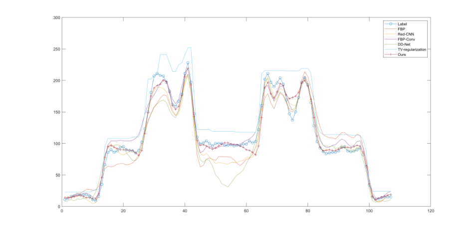
Fig. 7 depicts the intensity profiles at pixel positions of i = 356 and j from 211 to 317, corresponding to the green line in Fig. 5a. Through visual inspection, it can be observed that the intensity profile of our method is the most consistent to the label image in most locations. This comparison demonstrates the advantage of our method over the other post-processing CT reconstruction networks on edge and detail preservation.

IV-B Fan-beam

(a) Label

(b) FBP

(d) Red-CNN

(e) FBP-Conv

(f) DD-Net

(g) Ours

Fig. 9: The zoomed regions marked by the red box in Fig. 8a.

To reconstruct the CT images, we need to scan the object at least $180^{\circ}$ for parallel-beam geometry and $180^{\circ}$ +fan angles for fan-beam geometry. So, when the number of scanning angles is limited and the same, 150, the qualities of the reconstructed CT images from the parallel-beam CT are higher than those from the fan-beam CT. Therefore, for the 2D limited-angle CT image reconstruction, the parallel-beam geometry is superior over the fan-beam geometry. However, to verify the ability of our network to reconstruct CT images from fan-beam limited-angle sinograms, we still perform the fan-beam CT reconstruction experiments.

IV-B1 Data Preparation

The same 1500 full dose CT images (of size 512 $\times$ 512) from “the 2016 NIH-AAPM-Mayo Clinic Low Dose CT Grand Challenge” are used as the CT image labels $\varsigma^{label}$ , where 995 of them are used as the training set, another 5 of them are used as the validation set and the other 500 as the test set.

Since it needs more GPU memories to implement the Randon transform for the fan-beam geometry CT, we downsample the CT image labels to reduce their size to 256 $\times$ 256, i.e., we perform the fan-beam CT image reconstruction experiments on CT images of size 256 $\times$ 256.

The radius of the fan-beam geometry is set as $R=600$ . We use the Matlab function “fanbeam” to generate the sinogram labels $z^{label}$ of size $721\times 360$ , where 360 is the number of scanning angles corresponding to $\frac{\pi}{180}\times[0:1:359]$ and $721$ is the number of detectors corresponding to $\frac{\pi}{180}\times[-18:0.05:18]$ and $18^{\circ}$ is half of the fan angles. We downsample $z^{label}$ at scanning angles $\frac{\pi}{180}\times[0:1:149]$ to get the simulated limited-angle sinogram $g$ of size $150\times 721$ . The limited-angle sinogram $g$ is the input of our network and the reconstructed CT image from $g$ by the FBP algorithm is used as the initial guesses of CT images $u_{0}$ . For the compared networks, Red-CNN, FBP-Conv and DD-Net, the reconstructed CT image from $g$ by the FBP algorithm is also used as their inputs.

IV-B2 Parameter Setup

The parameters $\Theta_{\varsigma}^{n}$ and $\Theta_{z}^{n}$ in $Res_{\varsigma}^{n}(\cdot)$ and $Res_{z}^{n}(\cdot)$ of our network are automatically initialized by Tensorflow using the default values. The initial values of parameters $\Theta_{u}$ in $Merge_{u}^{n}(\cdot)$ are set as $t_{1}=1$ and $t_{2}=t_{3}=t_{4}=0.1$ . The number of iterations is set as $N_{iter}=3$ . The batch size is set as 2 and the number of training epochs is $100$ .

The parameters of the TV regularization algorithm for fan-beam CT are set as $\lambda_{3}=20$ , $\rho=0.1$ , $t_{5}=0.1$ , the number of maximal iterations $M_{iter}=300$ and the convergent criteria $\frac{\|u^{n+1}-u^{n}\|^{2}_{2}}{\|u^{n+1}\|^{2}_{2}}\leq\epsilon=10^{-4}$ .

IV-B3 Subjective Evaluation

Fig. 8 shows some reconstructed results from the test set by the six methods. It can be observed that the reconstructed images in Fig. 8b by the FBP algorithm have severe artifacts caused by the incomplete data. The results of the TV regularization algorithm still have some artifacts and some of the edges and structures in Fig. 8c are blurred. From Fig. 8d to Fig. 8g, we can observe that the artifacts are suppressed to different degrees by the different networks. However, the results of Red-CNN in Fig. 8d and DD-Net in Fig. 8f have some dark areas which are caused by the intensity inhomogeneous. The boundaries of the reconstructed images by the FBP-conv in Fig. 8e are somewhat blurred. Compared to these methods, the results of our method can preserve more fine edges and structures and have no inhomogeneous intensities.

To better demonstrate that our method can preserve more edges and boundaries, Fig. 9 shows the zoomed regions marked by the red box in Fig. 8a. It can be easily observed that the boundaries and edges of the reconstructed images by our method are the most consistent with the labels compared to those by the other methods.

(a) Label

(b) FDK

(d) FBP-Conv

(e) DD-Net

(f) Ours

Fig. 11: The zoomed regions marked by the red box in Fig. 10a.

IV-B4 Objective Evaluation

Quantitative analysis for the CT images reconstructed from the test set by the six methods has also been performed and the results are shown in Table II. It can be observed that our method has the highest SSIM and PSNR in average. Compared to the second highest, Red-CNN, the PSNR of our method is about 0.7db higher than it.

TABLE II: The Averaged PSNR and SSIM of CT Images Reconstructed by the Six Methods for Parallel-Beam CT

	PSNR	SSIM
FBP	15.43	0.51
TV regularization	26.95	0.84
Red-CNN	28.69	0.86
FBP-Conv	27.97	0.84
DD-Net	27.15	0.82
Ours	29.41	0.87

IV-C Circle Cone-beam

IV-C1 Data Preparation

The full dose CT images from “the 2016 NIH-AAPM-Mayo Clinic Low Dose CT Grand Challenge” are also used as the CT image labels $\varsigma^{label}$ . Due to the limitation of GPU memory, we choose only 4 continuous CT images and downsample them to form the object labels $\varsigma^{label}$ of size $64\times 64\times 4$ . We totally assemble 700 objects, where 596 of them are used as the training set, another 4 of them are used as the validation set and the other 100 as the test set.

The radius of the circle cone-beam geometry is set as $DSO=500$ , the distance between the X-ray source and the flat detector panel is set as $DSD=565$ . The size of the detector array is $79\times 7$ and the distances between each detector are $1$ . The objects are centrally located at the origin, where $[-32:31]\times[-32:31]$ corresponds to the $x-y$ coordinates and $[-2:1]$ corresponds to the z-coordinate. We obtain the sinogram labels $z^{label}$ by rotating the X-ray source in the $x-y$ plane along the $z$ coordinate to sample the object at angels $\frac{\pi}{180}\times[0:1:219]$ . Thus the size of the sinogram labels $z^{label}$ is $79\times 7\times 220$ . We downsample $z^{label}$ at scanning angles $\frac{\pi}{180}\times[0:1:179]$ to get the simulated limited-angle sinogram $g$ of size $79\times 7\times 180$ . The limited-angle sinogram $g$ is the input of our network and the reconstructed CT image from $g$ by the short-scan FDK [29] algorithm is used as the initial guesses of CT images $u_{0}$ . For the compared networks, Red-CNN, FBP-Conv and DD-Net, all slices of the reconstructed CT image from $g$ by the short-scan FDK algorithm are used as their inputs.

IV-C2 Parameter Setup

IV-C3 Subjective Evaluation

Fig. 10 shows four slices of one object from the test set by the five methods, FDK, Red-CNN, FBP-Conv, DD-Net and ours and Fig. 11 shows the zoomed regions marked by the red box in Fig. 10a. From Fig. 11, it can be observed that the contrast of the reconstructed images by our method is the most consistent with the labels compared to those by the other methods, which demonstrates that our method can preserve more edge information.

IV-C4 Objective Evaluation

The average PSNR and SSIM of the reconstructed CT image slices from the test set are listed in Table III. It can be observed that our method has the highest SSIM and PSNR in average. Compared to the second highest, DD-Net, the PSNR of our method is about 3.8db higher.

TABLE III: The Averaged PSNR and SSIM of CT Images Reconstructed by the five Methods for Circle Cone-Beam CT

	PSNR	SSIM
FDK	8.19	0.55
Red-CNN	30.10	0.89
FBP-Conv	29.15	0.89
DD-Net	30.22	0.82
Ours	34.04	0.91

V Conclusion

In this paper, we first proposed a variational model with two regularizations for the limited-angle CT image reconstruction, where one regularization utilizes the prior information of sinograms in the frequency domain and the other utilizes the prior information of CT images in the spatial domain. Then we used the penalty method to convert the variational model into three iterative subproblems, where the first subproblem completes the sinograms and the second refines the CT images, and the last merges the outputs of the first two subproblems. Instead of giving any explicit form of the regularizations and using the optimal algorithms to solve the first two subproblems, we used the CNNs of four layers to approximate the solutions of the first two subproblems. Therefore, by unrolling the iterative algorithm, we obtained an end-to-end deep network for the limited-angle CT image reconstruction. Experimental results showed that our deep network outperformed the existing algorithms under parallel-beam, fan-beam and circle cone-beam scanning geometries for the limited-angle CT image reconstruction.

References

[1] F. Matter, The Mathematics of Computerized Tomography. New York: John Wiley and Sons. Nemoz, 1986.
[2] H. Gao, L. Zhang, Z. Chen, Y. Xing, and J. Cheng, “An Extrapolation Method for Image Reconstruction from a Straight-line Trajectory,” in Proc. IEEE Nucl. Sci. Symp. Conf. Rec., 2006, pp. 2304–2308.
[3] M. DAVISON, “The Ill-Conditioned Nature of the Limited Angle Tomography Problem,” SIAM J. Appl. Math., vol. 43, no. 2, pp. 428–448, 1983.
[4] J. Frikel and E. T. Quinto, “Characterization and Reduction of Artifacts in Limited Angle Tomography,” Inverse Prob., vol. 29, no. 12, DEC 2013.
[5] E. QUINTO, “Singularities of the X-Ray Transform and Limited Data Tomography in R(2) and R(3) ,” SIAM J. Math. Anal., vol. 24, no. 5, pp. 1215–1225, SEP 1993.
[6] Z. Chen, X. Jin, L. Li, and G. Wang, “A Limited-Angle CT Reconstruction Method Based on Anisotropic TV Minimization,” Phys. Med. Biol., vol. 58, no. 7, pp. 2119–2141, APR 7 2013.
[7] T. Wang, K. Nakamoto, H. Zhang, and H. Liu, “Reweighted Anisotropic Total Variation Minimization for Limited-Angle CT Reconstruction,” IEEE Trans. Med. Imag., vol. 64, no. 10, pp. 2742–2760, OCT 2017.
[8] E. Y. Sidky and X. Pan, “Image Reconstruction in Circular Cone-Beam Computed Tomography By Constrained, Total-Variation Minimization,” Phys. Med. Biol., vol. 53, no. 17, pp. 4777–4807, SEP 7 2008.
[9] L. Ritschl, F. Bergner, C. Fleischmann, and M. Kachelriess, “Improved Total Variation-Based CT Image Reconstruction Applied To Clinical Data,” Phys. Med. Biol., vol. 56, no. 6, pp. 1545–1561, MAR 21 2011.
[10] R. Tovey, M. Benning, C. Brune, M. J. Lagerwerf, S. M. Collins, R. K. Leary, P. A. Midgley, and C.-B. Schonlieb, “Directional Sinogram Inpainting for Limited Angle Tomography,” Inverse Prob., vol. 35, no. 2, FEB 2019.
[11] J. Yang, H. Yu, M. Jiang, and G. Wang, “High-Order Total Variation Minimization for Interior Tomography,” Inverse Prob., vol. 26, no. 3, MAR 2010.
[12] Y. Liu, Z. Liang, J. Ma, H. Lu, K. Wang, H. Zhang, and W. Moore, “Total Variation-Stokes Strategy for Sparse-View X-ray CT Image Reconstruction,” IEEE Trans. Med. Imag., vol. 33, no. 3, pp. 749–763, MAR 2014.
[13] M. Rantala, S. Vanska, S. Jarvenpaa, M. Kalke, M. Lassas, J. Moberg, and S. Siltanen, “Wavelet-Based Reconstruction for Limited-Angle X-Ray Tomography,” IEEE Trans. Med. Imag., vol. 25, no. 2, pp. 210–217, FEB 2006.
[14] R. Zhan and B. Dong, “CT Image Reconstruction by Spatial-Radon Domain Data-Driven Tight Frame Regularization,” SIAM J. Imag. Sci., vol. 9, no. 3, pp. 1063–1083, 2016.
[15] Zhang Tao, Wang Bin, Yang Li-juan, and Qi Nai-xin, “Low Dose CT Image Enhancement Based on Second Generation Curvelet Transform,” Comput. Eng. Appl., vol. 46, pp. 191–3, Feb. 2010.
[16] B. Vandeghinste, B. Goossens, R. Van Holen, C. Vanhove, A. Pizurica, S. Vandenberghe, and S. Staelens, “Iterative CT Reconstruction Using Shearlet-Based Regularization,” IEEE Trans. Nucl. Sci., vol. 60, no. 5, 1, pp. 3305–3317, OCT 2013.
[17] Q. Xu, H. Yu, X. Mou, L. Zhang, J. Hsieh, and G. Wang, “Low-Dose X-ray CT Reconstruction via Dictionary Learning,” IEEE Trans. Med. Imag., vol. 31, no. 9, pp. 1682–1697, SEP 2012.
[18] Y. Lu, J. Zhao, and G. Wang, “Few-View Image Reconstruction With Dual Dictionaries,” Phys. Med. Biol., vol. 57, no. 1, pp. 173–189, JAN 7 2012.
[19] Y. Huang, Y. Lu, O. Taubmann, G. Lauritsch, and A. Maier, “Traditional Machine Learning for Limited Angle Tomography,” Int. J. Comput. Assist. Radiol. Surg., vol. 14, no. 1, pp. 11–19, JAN 2019.
[20] T. Wüerfl, M. Hoffmann, V. Christlein, K. Breininger, Y. Huang, M. Unberath, and A. K. Maier, “Deep Learning Computed Tomography: Learning Projection-Domain Weights From Image Domain in Limited Angle Problems,” IEEE Trans. Med. Imag., vol. 37, no. 6, SI, pp. 1454–1463, JUN 2018.
[21] Y. Huang, S. Wang, Y. Guan, and A. Maier, “Limited Angle Tomography for Transmission X-Ray Microscopy Using Deep Learning,” J. Synchrotron Radiat., vol. 27, no. 2, pp. 477–485, MAR 2020.
[22] R. Anirudh, H. Kim, J. J. Thiagarajan, K. A. Mohan, K. Champley, and T. Bremer, “Lose the Views: Limited Angle CT Reconstruction via Implicit Sinogram Completion,” in Proc. CVPR, 2018, pp. 6343–6352.
[23] T. A. Bubba, G. Kutyniok, M. Lasses, M. Maerz, W. Samek, S. Siltanen, and V. Srinivasan, “Learning the Invisible: A Hybrid Deep Learning-Shearlet Framework For Limited Angle Computed Tomography,” Inverse Prob., vol. 35, no. 6, JUN 2019.
[24] Z. Li, W. Zhang, L. Wang, A. Cai, N. Liang, B. Yan, and L. Li, “A Sinogram Inpainting Method Based on Generative Adversarial Network For Limited-Angle Computed Tomography,” in 15th International Meeting on Fully Three-dimensional Image Reconstruction in Radiology and Nuclear Medicine, vol. 11072, 2019.
[25] M. Ghani and W. Karl, “Integrating Data and Image Domain Deep Learning for Limited Angle Tomography using Consensus Equilibrium,” in Proc. ICCVW, 2019, pp. 3922–32.
[26] R. SIDDON, “Fast Calculation of the Exact Radiological Path for a 3-dimensional CT Array,” Med. Phys., vol. 12, no. 2, pp. 252–255, 1985.
[27] J. He, Y. Yang, Y. Wang, D. Zeng, Z. Bian, H. Zhang, J. Sun, Z. Xu, and J. Ma, “Optimizing a Parameterized Plug-and-Play ADMM for Iterative Low-Dose CT Reconstruction,” IEEE Trans. Med. Imag., vol. 38, no. 2, pp. 371–382, FEB 2019.
[28] H. Gao, “Fused Analytical and Iterative Reconstruction (air) Via Modified Proximal Forward-backward Splitting: A Fdk-based Iterative Image Reconstruction Example for Cbct,” Phys. Med. Biol., vol. 61, no. 19, pp. 7187–7204, OCT 7 2016.
[29] G. WANG, Y. LIU, T. LIN, and P. CHENG, “Half-Scan Cone-Beam X-Ray Microtomography Formula,” SCANNING, vol. 16, no. 4, pp. 216–220, 1994.
[30] H. Chen, Y. Zhang, M. K. Kalra, F. Lin, Y. Chen, P. Liao, J. Zhou, and G. Wang, “Low-Dose CT With a Residual Encoder-Decoder Convolutional Neural Network,” IEEE Trans. Med. Imag., vol. 36, no. 12, pp. 2524–2535, 2017.
[31] K. H. Jin, M. T. McCann, E. Froustey, and M. Unser, “Deep Convolutional Neural Network for Inverse Problems in Imaging,” IEEE Trans. Image Process., vol. 26, no. 9, pp. 4509–4522, 2017.
[32] Z. Zhang, X. Liang, X. Dong, Y. Xie, and G. Cao, “A Sparse-View CT Reconstruction Method Based on Combination of DenseNet and Deconvolution,” IEEE Trans. Med. Imag., vol. 37, no. 6, SI, pp. 1407–1417, 2018.
[33] H. Gupta, K. H. Jin, H. Q. Nguyen, M. T. McCann, and M. Unser, “CNN-Based Projected Gradient Descent for Consistent CT Image Reconstruction,” IEEE Trans. Med. Imag., vol. 37, no. 6, SI, pp. 1440–1453, JUN 2018.
[34] S. Boyd, N. Parikh, E. Chu, B. Peleato, and J. Eckstein, “Distributed Optimization and Statistical Learning via the Alternating Direction Method of Multipliers,” Founds. Trends Mach. Learn., vol. 3, pp. 1–122, 2010.
[35] C. McCollough, “TU-FG-207A-04: Overview of the Low Dose CT Grand Challenge,” Med. Phys., vol. 43, no. 3759-3760, pp. 3759–3760, 2016.

$\displaystyle\\|u\\|_{\mathrm{RwATV}}=$	$\displaystyle\left\\|R\nabla_{A,B}u\right\\|_{1}=\sum_{i,j}r_{i,j}\left\|\nabla_{A,B}u_{i,j}\right\|,$	(8)
$\displaystyle r_{i,j}^{(l+1)}=$	$\displaystyle\frac{1}{\left\|\nabla_{A,B}u_{i,j}^{(l)}\right\|+\xi},$
$\displaystyle\left\|\nabla_{A,B}u_{i,j}\right\|=$	$\displaystyle\sqrt{A\left(u_{i,j}-u_{i-1,j}\right)^{2}+B\left(u_{i,j}-u_{i,j-1}\right)^{2}},$

A model-guided deep network for limited-angle computed tomography

Abstract

Index Terms:

I Introduction

II Preliminaries and Related works

II-A CT Reconstruction Model

II-B Related Works

III Proposed model and Network

III-A Proposed Model

III-B Proposed Network

III-B1 Structure of Sub-network R​e​sςn​(⋅)Res_{\varsigma}^{n}(\cdot) for Updating ς\varsigma

III-B2 Structure of Sub-network R​e​szn​(⋅)Res_{z}^{n}(\cdot) for Updating zz

III-B3 Structure of Sub-network M​e​r​g​eun⁡(⋅)\mathop{Merge}_{u}^{n}(\cdot) for Updating uu

III-C Interpretability and Consistency

III-C1 Interpretability

III-C2 Consistency

III-D Loss Function

IV Experimental Results

IV-A Parallel-beam

IV-A1 Data Preparation

IV-A2 Parameter Setup

IV-A3 Subjective Evaluation

IV-A4 Objective Evaluation

IV-B Fan-beam

IV-B1 Data Preparation

IV-B2 Parameter Setup

IV-B3 Subjective Evaluation

IV-B4 Objective Evaluation

IV-C Circle Cone-beam

IV-C1 Data Preparation

IV-C2 Parameter Setup

IV-C3 Subjective Evaluation

IV-C4 Objective Evaluation

V Conclusion

References

III-B1 Structure of Sub-network $Res_{\varsigma}^{n}(\cdot)$ for Updating $\varsigma$

III-B2 Structure of Sub-network $Res_{z}^{n}(\cdot)$ for Updating $z$

III-B3 Structure of Sub-network $\mathop{Merge}_{u}^{n}(\cdot)$ for Updating $u$